Information Theoretic Hierarchical Clustering

Abstract

Hierarchical clustering has been extensively used in practice, where clusters can be assigned and analyzed simultaneously, especially when estimating the number of clusters is challenging. However, due to the conventional proximity measures recruited in these algorithms, they are only capable of detecting mass-shape clusters and encounter problems in identifying complex data structures. Here, we introduce two bottom-up hierarchical approaches that exploit an information theoretic proximity measure to explore the nonlinear boundaries between clusters and extract data structures further than the second order statistics. Experimental results on both artificial and real datasets demonstrate the superiority of the proposed algorithm compared to conventional and information theoretic clustering algorithms reported in the literature, especially in detecting the true number of clusters.

1. Introduction

Clustering is an unsupervised approach for segregating data into its natural groups, such that the samples in each group have the highest similarity with each other and the highest dissimilarity with samples of the other groups. Clustering is in general exploited when labeling data by a human operator is expensive and subject to error, and has many applications in data mining, image segmentation, remote sensing, and compression, to name but a few.

One of the main characteristics of any clustering algorithm is its definition of proximity measure. Various clustering algorithms have different notions of proximity. For instance, measures such as the Euclidean distance or the within cluster variance, also referred to as the Mahalanobis distance [1], can explore up to the second order statistics of the data. Determining an appropriate proximity measure for clustering is a challenging task that directly depends on the structure of the data. With an ill-defined proximity measure, even compatible clustering algorithms fail in accurately identifying the data structures. Since conventional clustering algorithms exploit within cluster variance measures, they are only capable of identifying spherical mass-shaped clusters, while complicated shapes are disregarded. Algorithms such as k-means [2], fuzzy c-means [3], divisive and agglomerative hierarchical clustering [4] fall into this category. On the other hand, clustering based on artificial neural networks [5] and support vector machines [6] can identify clusters with various shapes, however, are computationally expensive and require perfect tunings.

Information theoretic measures have been proposed as proximity measures that can extract data structures further than the second order statistics [7,8]. However, practical difficulties in estimating the distribution of data have significantly reduced the applicability of such proximity measures in clustering, especially when no prior information about the data structures is given. The distribution can be estimated by either parametric models, such as a mixture of Gaussian functions [9], or bynon-parametric models, such as the Parzen window estimator [10]. Regardless of the model used for estimating the distribution, the performance of any information theoretic clustering totally depends on how well the estimator predicts this distribution, its computational cost, and its ability in updating the distribution as the clustering proceeds.

Information theoretic clustering algorithms have tackled the challenges of estimating the distribution from different prospects. Mutual information, defined using either the Shannon’s or Kolmogorov’s interpretation of information, has been used for combining clusters in an agglomerative hierarchical clustering, in which the distribution is approximated using the k-nearest neighbor estimator [11]. Using the grid and count method for estimating the distribution, the statistical correlation among clusters was minimized for clustering gene-wide expression data [12]. The k-nearest neighbor estimator is sub-optimal in the sense that it requires re-estimating the distribution after the clusters are updated. Although the grid and count method benefits from updating the distribution of combined clusters from the existing ones, but this algorithm produces biased estimations for small-sized high-dimensional data.

In this paper, the distribution is estimated using a Parzen window estimator with Gaussian kernels centered on each sample and with a constant covariance. Although this distribution seems superficial and computationally expensive, but exploiting the Rényi’s entropy estimator [13] in a quadratic form as the proximity measure, the mutual information can be estimated from pairwise distances, also referred to as the quadratic mutual information [14]. This proximity measure has been used in an iterative clustering to optimize the clustering evaluation function that will find the nonlinear boundaries between clusters [15]. It also has been used in learning the discriminant transform from the mutual information estimated between the cluster labels and the transformed features for classification [16]. Here, we use a similar technique in finding the association between the data samples and cluster labels using the quadratic mutual information. We will show how increasing the quadratic mutual information assigns appropriate clusters to the data.

First, by introducing the clustering as a distortion-rate problem, we will show how optimizing the distortion-rate function provides us with the best clustering result. We propose a hierarchical approach for this optimization. Unlike partitioning approaches such as k-means clustering that primarily require setting the number of clusters, the hierarchical approach gives us the additional ability of detecting the number of clusters in data, especially when no prior information is available. Starting from an initial set of clusters generated by a simple clustering algorithm, in each hierarchy, a cluster is eliminated and merged with the remaining clusters, until one cluster remains. Eventually, based on the variations in the mutual information, the true number of clusters is determined.

We propose two algorithms for the hierarchical optimization, the agglomerative and the split-and-merge clustering. In the former, at any hierarchy, the two clusters that maximize the mutual information are combined into one cluster. In the latter one, a cluster that has the worst effect on the mutual information is singled out for elimination. This cluster is split and its samples are allocated to the remaining clusters. Both these methods maximize the mutual information and have advantages compared to one another. In the following section, we will first demonstrate how optimizing the distortion-rate function provides us with the best clustering and then show how the mutual information can be approximated by the quadratic mutual information. The two hierarchical approaches are also demonstrated in this section. In Section 3, we will demonstrate the performance of the proposed hierarchical clustering on both artificial and real datasets, and will compare them with clustering algorithms reported in the literature.

2. Theory

2.1. Distortion-Rate Theory

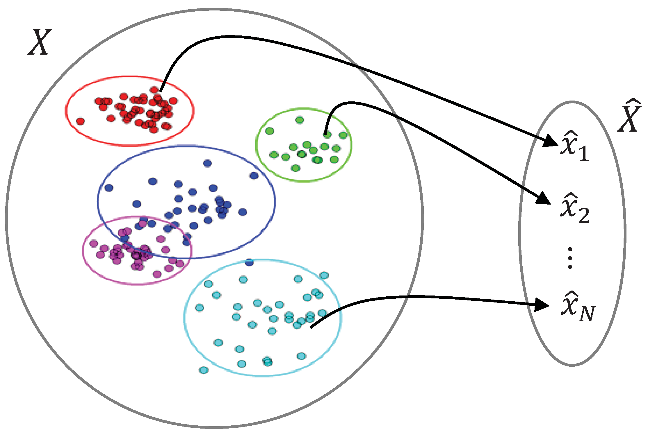
Clustering can be viewed as projecting a large number of discrete samples from the input space, into a finite set of discrete symbols in the clustered space, where each symbol resembles a cluster. Thus, clustering is a many-to-one mapping from the input space, $X$, to the clustered space, $\widehat{X}$, and can be fully characterized by the conditional probability distribution, $p(\widehat{x}|x)$. Using this mapping, the distribution of the clustered space is estimated as:

$$p\left(\widehat{x}\right)={\displaystyle \sum }_{x\in X}p\left(x\right)p\left(\widehat{x}\text{|}x\right)$$

(1)

where $p\left(x\right)$ is the distribution of the input space. Figure 1 demonstrates a many-to-one mapping, where each symbol, ${\widehat{x}}_i\in \widehat{X}$, for $i=1,2,\dots ,N$, represents a cluster of samples from the input space, and $N$ is the number of clusters.

Although clusters have different number of samples, but the average number of samples in each cluster is $2^{H\left(\widehat{X}\text{|}X\right)}$, where $H\left(\widehat{X}\text{|}X\right)$ is the conditional entropy of the clustered space given the input space and is estimated as:

$$H\left(\widehat{X}\text{|}X\right)={\displaystyle \sum }_{x\in X}{\displaystyle \sum }_{\widehat{x}\in \widehat{X}}p\left(x\right)p\left(\widehat{x}\text{|}x\right)\log p\left(\widehat{x}\text{|}x\right)$$

(2)

The number of clusters is $2^{H\left(\widehat{X}\right)}$, where $H\left(\widehat{X}\right)$ is the entropy of the clustered space. Note that $H\left(\widehat{X}\right)$ is upper bounded by $\log N$ and is equal to the upper bound only when all clusters have an equal number of samples.

Figure 1. Demonstration of a many-to-one mapping from the input space, includingsemi-infinite number of discrete samples, to a finite number of symbols, $N$, in the clustered space.

Figure 1. Demonstration of a many-to-one mapping from the input space, includingsemi-infinite number of discrete samples, to a finite number of symbols, $N$, in the clustered space.

To obtain a lossless many-to-one mapping, the immediate goal is to preserve the information in $X$ in the projected space, $\widehat{X}$. The loss of information due to mapping is measured by the conditional entropy, $H\left(X\text{|}\widehat{X}\right)=H\left(X\right)-I\left(X;\widehat{X}\right)$, where $H\left(X\right)$ is the amount of information in $X$. The mutual information between the input and clustered space, $I\left(X;\widehat{X}\right)$, is estimated as:

$$I\left(X;\widehat{X}\right)={\displaystyle \sum }_{x\in X}{\displaystyle \sum }_{\widehat{x}\in \widehat{X}}p\left(x,\widehat{x}\right)\log \frac{p\left(x,\widehat{x}\right)}{p\left(x\right)p\left(\widehat{x}\right)}={\displaystyle \sum }_{x\in X}{\displaystyle \sum }_{\widehat{x}\in \widehat{X}}p\left(x\right)p\left(\widehat{x}\text{|}x\right)\log \frac{p\left(\widehat{x}\text{|}x\right)}{{{\displaystyle \sum }}_{x\in X}p\left(x\right)p\left(\widehat{x}\text{|}x\right)}$$

(3)

Notice how the mutual information is estimated based on only the input distribution, $p\left(x\right)$, and mapping distribution, $p\left(\widehat{x}\text{|}x\right)$. Mutual information gives us the rate by which the clustered space represents the input space. For a lossless mapping, $H\left(X\text{|}\widehat{X}\right)=0$ or $I\left(X;\widehat{X}\right)=H\left(X\right)$, which in turn means that all the information in the input space is sent to the clustered space. While a higher rate for the clustered space generates less information loss, reducing this rate increases the information loss, therefore introducing a tradeoff between the rate and the information loss. In clustering, the goal is to introduce a lossy many-to-one mapping that reduces the rate by representing the semi-infinite input space with a finite number of clusters, thus introducing information loss such that $I\left(X;\widehat{X}\right)\le H\left(X\right)$.

The immediate goal in clustering is to introduce clusters with the highest similarity or lowest distortion among its samples. Distortion is the expected value of the distance between the input and clustered spaces, $d\left(x,\widehat{x}\right)$, defined based on the joint distribution, $p\left(x,\widehat{x}\right)$, as:

$$E_{p\left(x,\widehat{x}\right)}\left[d\left(x,\widehat{x}\right)\right]={\displaystyle \sum }_{x\in X}{\displaystyle \sum }_{\widehat{x}\in \widehat{X}}p\left(x,\widehat{x}\right)d\left(x,\widehat{x}\right)$$

(4)

Different proximity measures can be defined as distortion, for instance, for the Euclidean distance, $\widehat{x}$ are the center of clusters and $d\left(x,\widehat{x}\right)={\displaystyle \sum }_{x\in X}{\left(x-\widehat{x}\right)}^2$ is the cluster variance and $p\left(x,\widehat{x}\right)=\frac{1}{Z}I\left(x\subset \widehat{x}\right)$ is a uniform distribution, where $Z={\displaystyle \sum }_{\widehat{x}\in \widehat{X}}p\left(x,\widehat{x}\right)$ is the normalizing term and $I(.)$ 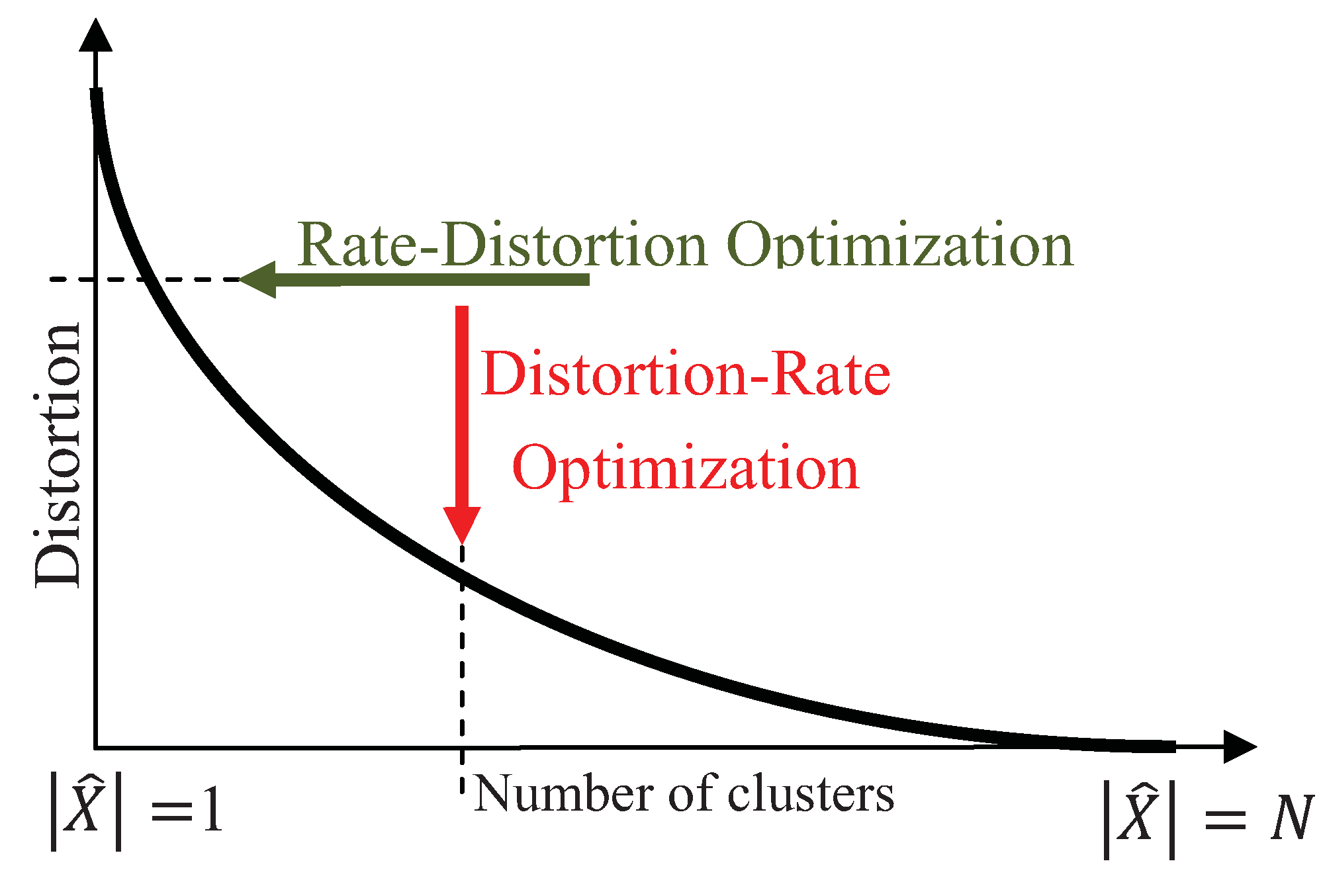is the indicator function. The tradeoff between the preserved amount of information and the expected distortion is characterized by the Shannon-Kolmogorov rate-distortion function, where the goal is to achieve the minimum rate for a given distortion, illustrated by the horizontal arrow in Figure 2. The rate-distortion optimization has been extensively used for quantization, where the goal is to achieve the minimum rate for a desired distortion [17]. Unlike quantization, the goal in clustering is to minimize the distortion for a preferred number of clusters, $N$, thus, the distortion-rate function is optimized instead:

$$D\left(R\right)=\underset{I\left(X;\widehat{X}\right)\le R}{\min }E\left[d\left(x,\widehat{x}\right)\right]$$

(5)

In Figure 2, the vertical arrow demonstrates the distortion-rate optimization that achieves the lowest distortion for a desired rate. Note that the number of clusters, $N$, places an upper bound on the rate, determined by the mutual information. Assuming that decreasing distortion monotonically increases the mutual information, clustering can be interpreted as maximizing the mutual information for a fixed number of clusters, $\widehat{X}=\underset{\left|\widehat{X}\right|=N}{\max }I\left(X;\widehat{X}\right)$, where $\left|\widehat{X}\right|$ is the number of clusters.

Figure 2. Demonstration of the rate-distortion and distortion-rate optimizations by the horizontal and vertical arrows, respectively.

Figure 2. Demonstration of the rate-distortion and distortion-rate optimizations by the horizontal and vertical arrows, respectively.

2.2. Quadratic Mutual Information

The Shannon’s mutual information estimates the distance between the joint distribution, $p_{XY}\left(x,y\right)$, and the product of the marginal distributions, $p_X\left(x\right)p_Y\left(y\right)$, [18], as:

$$I\left(X;Y\right)=\underset{X}{{\displaystyle \int }}\underset{Y}{{\displaystyle \int }}{p}_{XY}\left(x,y\right)\log \frac{p_{XY}\left(x,y\right)}{p_X\left(x\right)p_Y\left(y\right)}dxdy$$

(6)

The mutual information has also been referred to as the Kullback-Leibler divergence between $p_{XY}\left(x,y\right)$ and $p_X\left(x\right)p_Y\left(y\right)$ [19]. Due to the challenges in estimating the Shannon’s mutual information, the Euclidean distance between $p_{XY}\left(x,y\right)$ and $p_X\left(x\right)p_Y\left(y\right)$ can be used instead as an approximation for mutual information, $\tilde{I}\left(X;Y\right)$, also referred to as the quadratic divergence between distributions [20]:

$$\begin{array}{c}\tilde{I}\left(X;Y\right)=\underset{X}{{\displaystyle \int }}\underset{Y}{{\displaystyle \int }}{\left(p_{XY}\left(x,y\right)-p_X\left(x\right)p_Y\left(y\right)\right)}^{2}dxdy\\ =\underset{X}{{\displaystyle \int }}\underset{Y}{{\displaystyle \int }}{p}_{XY}^2\left(x,y\right)dxdy-2\underset{X}{{\displaystyle \int }}\underset{Y}{{\displaystyle \int }}{p}_{XY}\left(x,y\right)p_X\left(x\right)p_Y\left(y\right)dxdy+\underset{X}{{\displaystyle \int }}{p}_X^2\left(x\right)dx\underset{X}{{\displaystyle \int }}{p}_Y^2\left(y\right)dy\end{array}$$

(7)

Considering the quadratic Rényi’s entropy estimator, $H_2\left(X\right)=-\ln {{\displaystyle \int }}^{\text{}}{f}^2\left(x\right)dx$, this entropy also includes the quadratic form of the distribution, $f\left(x\right)$. Note that the quadratic Rényi’s entropy estimator is the second order, $\alpha =2$, of the Rényi’s entropy estimator, $H_{\alpha }\left(X\right)=\frac{1}{1-\alpha }\ln {{\displaystyle \int }}^{\text{}}{f}^{\alpha }\left(x\right)dx$ [13]. By disregarding the logarithm in the quadratic Rényi’s entropy, the quadratic approximation of mutual information in (7) is a valid estimator of the information content, and indeed can be used for clustering.

2.3. Parzen Window Estimator with Gaussian Kernels

The distribution of samples in cluster $\mathcal{X}$ is approximated by the non-parametric Parzen window estimator with Gaussian kernels [21,22], in which a Gaussian function is centered on each sample as:

$$p_X\left(x\right)=\frac{1}{\left|\mathcal{X}\right|}{\displaystyle \sum }_{i=1}^{\left|\mathcal{X}\right|}\frac{1}{\sqrt{{\left(2\pi \right)}^d\left|\Sigma \right|}}exp\left(-\frac{1}{2}{\left(x-x_i\right)}^T{\Sigma }^{-1}\left(x-x_i\right)\right)$$

(8)

where $T$ is transpose, $d$ is the dimension of $x$, $\Sigma$ is the covariance matrix, $x_i\in \mathcal{X}$ are the samples of cluster $\mathcal{X}$, and the cardinality $\left|\mathcal{X}\right|$ is the number of samples in that cluster. Assuming the variances for different dimensions are equal and independent from each other, thus, providing us with a diagonal covariance matrix with constant elements, ${\delta }_X^2$, the distribution is simplified as:

$$p_X\left(x\right)=\frac{1}{\left|\mathcal{X}\right|}{\displaystyle \sum }_{i=1}^{\left|\mathcal{X}\right|}\frac{1}{\sqrt{{\left(2\pi {\delta }_X^2\right)}^d}}exp\left(-\frac{{\left(x-x_i\right)}^2}{2{\delta }_X^2}\right)=\frac{1}{\left|\mathcal{X}\right|}{\displaystyle \sum }_{i=1}^{\left|\mathcal{X}\right|}\mathcal{N}\left(x-x_i,{\delta }_X^2\right)$$

(9)

where $\mathcal{N}\left(\mu ,{\delta }^2\right)$ is a Gaussian function with mean $\mu$ and variance ${\delta }^2$. Using the distribution estimator in (9), the quadratic terms in (7) can be further simplified as:

$$\begin{array}{ll}\underset{X}{{\displaystyle \int }}{p}_X^2\left(x\right)dx=& \frac{1}{\left|{\mathcal{X}}_k\right|}\frac{1}{\left|{\mathcal{X}}_l\right|}{\displaystyle \sum _{i=1}^{\left|{\mathcal{X}}_k\right|}}{\displaystyle \sum _{j=1}^{\left|{\mathcal{X}}_l\right|}}\underset{X}{{\displaystyle \int }}\mathcal{N}\left(x-x_i,{\delta }_X^2\right)\mathcal{N}\left(x-x_j,{\delta }_X^2\right)dx\\ & =\frac{1}{\left|{\mathcal{X}}_k\right|}\frac{1}{\left|{\mathcal{X}}_l\right|}{\displaystyle \sum _{i=1}^{\left|{\mathcal{X}}_k\right|}}{\displaystyle \sum _{j=1}^{\left|{\mathcal{X}}_l\right|}}\mathcal{N}\left(x_i-x_j,2{\delta }_X^2\right)\end{array}$$

(10)

where $x_i\in {\mathcal{X}}_k$ and $x_j\in {\mathcal{X}}_l$ are the samples from clusters ${\mathcal{X}}_k$ and ${\mathcal{X}}_l$, respectively, and $\left\{{\mathcal{X}}_k,{\mathcal{X}}_l\right\}\in \widehat{X}$ are clusters from the clustered space. Note that the convolution of two Gaussian functions is also a Gaussian function.

Back to the clustering problem, in which the input space is the individual samples and clustered space is the finite number of clusters, the quadratic mutual information in (7) is restructured in the following discrete form:

$$\begin{array}{c}\tilde{I}\left(X;\widehat{X}\right)={\displaystyle \sum _{x\in X}}{\displaystyle \sum _{\widehat{x}\in \widehat{X}}}{\left(p_{X\widehat{X}}\left(x,\widehat{x}\right)-p_X\left(x\right)p_{\widehat{X}}\left(\widehat{x}\right)\right)}^2\\ ={\displaystyle \sum _{x\in X}}{\displaystyle \sum _{\widehat{x}\in \widehat{X}}}{p}_{X\widehat{X}}^2\left(x,\widehat{x}\right)-2{\displaystyle \sum _{x\in X}}{\displaystyle \sum _{\widehat{x}\in \widehat{X}}}{p}_{X\widehat{X}}\left(x,\widehat{x}\right)p_X\left(x\right)p_{\widehat{X}}\left(\widehat{x}\right)+{\displaystyle \sum _{x\in X}}{\displaystyle \sum _{\widehat{x}\in \widehat{X}}}{p}_X^2\left(x\right)p_{\widehat{X}}^2\left(\widehat{x}\right)\end{array}$$

(11)

The distribution of data, $p_X\left(x\right)$, is equal to the distribution of all samples considered as one cluster, and is estimated using (9) as:

$$p_X\left(x\right)=\frac{1}{\left|X\right|}{\displaystyle \sum }_{i=1}^{\left|X\right|}\mathcal{N}\left(x-x_i,{\delta }_X^2\right)$$

(12)

where $\left|X\right|$ is the total number of samples, $\left|X\right|={\displaystyle \sum }_{k=1}^N\left|{\mathcal{X}}_k\right|$, and $\left|{\mathcal{X}}_k\right|$ is the number of samples in the $k^{th}$ cluster, $\left\{{\mathcal{X}}_k\right\}\in \widehat{X}$. The distribution of the clustered space, on the other hand, is estimated as:

$$p_{\widehat{X}}\left(\widehat{x}\right)=\frac{\left|{\mathcal{X}}_k\right|}{\left|X\right|} for k=1,\dots ,N$$

(13)

The joint distribution, $p_{X\widehat{X}}\left(x,\widehat{x}\right)$, for each of the $N$ clusters of the clustered space is estimated as:

$$p_{X\widehat{X}}\left(x,\widehat{x}\right)=p\left(x|\widehat{x}\right)p_{\widehat{X}}\left(\widehat{x}\right)=\frac{1}{\left|X\right|}{\displaystyle \sum }_{i=1}^{\left|{\mathcal{X}}_k\right|}\mathcal{N}\left(x-x_i,{\delta }_X^2\right) for k=1,\dots ,N$$

(14)

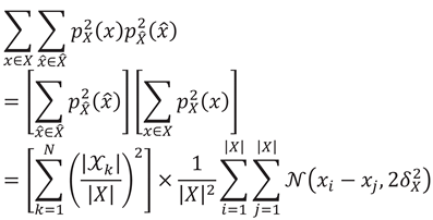
Substituting (12), (13) and (14) in (11) provides us with the following approximation for the discrete quadratic mutual information (proof provided in Appendix):

(15)

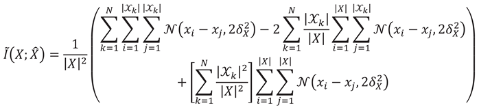
For simplification, here we define the between cluster distance among clusters ${\mathcal{X}}_k$ and ${\mathcal{X}}_l$, as ${\delta }_{k,l}={\displaystyle \sum }_{i=1}^{\left|{\mathcal{X}}_k\right|}{\displaystyle \sum }_{j=1}^{\left|{\mathcal{X}}_l\right|}\mathcal{N}\left(x_i-x_j,2{\delta }_X^2\right)$, therefore, (15) can be represented as:

$$\tilde{I}\left(X;\widehat{X}\right)=\frac{1}{{\left|X\right|}^2}\left({\displaystyle \sum }_{k=1}^N{\delta }_{k,k}-2{\displaystyle \sum }_{k=1}^N\frac{\left|{\mathcal{X}}_k\right|}{\left|X\right|}{\displaystyle \sum }_{l=1}^N{\delta }_{k,l}+\kappa {\displaystyle \sum }_{k=1}^N\frac{{\left|{\mathcal{X}}_k\right|}^2}{{\left|X\right|}^2}\right)$$

(16)

where $\kappa ={\displaystyle \sum }_{i=1}^{\left|X\right|}{\displaystyle \sum }_{j=1}^{\left|X\right|}\mathcal{N}\left(x_i-x_j,2{\delta }_X^2\right)$ is a constant.

2.4. Hierarchical Optimization

The proposed hierarchical algorithm, similar to most hierarchical clustering algorithms, operates in a bottom-up approach. In this approach clusters are merged together until one cluster is obtained, and then the whole process is evaluated to find the best number of clusters that fits the data [4]. Such clustering algorithms start by assuming each sample as an individual cluster, and therefore require $\left|X\right|-1$ merging steps. To reduce the number of merging steps, hierarchical algorithms generally exploit an low-complexity initial clustering, such as k-means clustering, to generate $\overline{N}$ clusters, far beyond the expected number of clusters in the data, but still much smaller than the number of samples, $\overline{N}\ll \left|X\right|$ [23,24]. The initial clustering generates small spherical clusters, while significantly reducing the computational complexity of the hierarchical clustering.

Similarly, in the proposed hierarchical algorithms, clusters are merged; however, the criterion is to maximize the quadratic mutual information. Here we propose two approaches for merging, the agglomerative clustering and the split and merge clustering. In each hierarchy of the agglomerative clustering, two clusters are merged into one cluster to maximize the quadratic mutual information. In each hierarchy of the split and merge clustering, on the other hand, the cluster that has the worst effect on the quadratic mutual information is first eliminated, and then its samples are assigned to the remaining clusters in the clustered space. Following, these two approaches are explained in details.

2.4.1. Agglomerative Clustering

In this approach, we compute the changes in the quadratic mutual information after combining any pair of clusters to find the best two clusters for merging. We pick the pair that generates the largest increase in the quadratic mutual information. Since, at each hierarchy, clusters with the lowest distortion are generated, therefore, this approach can be used for optimizing the distortion-rate function in (5). Assuming that clusters ${\mathcal{X}}_A$ and ${\mathcal{X}}_B$ are merged to produce ${\mathcal{X}}_C={\mathcal{X}}_A{{\displaystyle \cup }}^{\text{}}{\mathcal{X}}_B$, the changes in the quadratic mutual information, $\mathrm{∆}{\tilde{I}}_{A,B}$, can be estimated as:

$$\begin{array}{ll}\mathrm{∆}{\tilde{I}}_{A,B}^{\left(t+1\right)}={\tilde{I}}^{\left(t+1\right)}& \left(X;\widehat{X}\right)-{\tilde{I}}^{\left(t\right)}\left(X;\widehat{X}\right)\\ & =\frac{1}{{\left|X\right|}^2}\left(2{\delta }_{A,B}-\frac{2}{\left|X\right|}\left(\left|{\mathcal{X}}_A\right|{\displaystyle \sum _{l=1}^N}{\delta }_{B,l}+\left|{\mathcal{X}}_B\right|{\displaystyle \sum _{l=1}^N}{\delta }_{A,l}\right)+\frac{2\kappa \left|{\mathcal{X}}_A\right|\left|{\mathcal{X}}_B\right|}{{\left|X\right|}^2}\right)\end{array}$$

(17)

where ${\tilde{I}}^{\left(t\right)}\left(X;\widehat{X}\right)$ is the quadratic mutual information at the step $t$. The closed form equation in (17) provides us with the best pair for merging without literally combining each pair and estimating the quadratic mutual information. Eventually, the maximum $\mathrm{∆}{\tilde{I}}_{A,B}^{\left(t+1\right)}$ at each hierarchy determines the true number of clusters in the data. Table 1 introduces the pseudo code for the agglomerative clustering approach.

Table 1. Pseudo code for the agglomerative clustering.

1: Initial Clustering, $\left|\widehat{X}\right|=\overline{N}$

2: for $t=1: \overline{N}-1$ do

3: Estimate $\mathrm{∆}{\tilde{I}}_{A,B}^{\left(t+1\right)}$ for all pairs

4: Merge clusters ${\mathcal{X}}_A$ and ${\mathcal{X}}_B$, in which ${\mathcal{X}}_A,{\mathcal{X}}_B={\max }_{A,B}\mathrm{∆}{\tilde{I}}_{A,B}^{\left(t+1\right)}$

5: end for

6: Determine # of clusters

Table 1. Pseudo code for the agglomerative clustering.

1: Initial Clustering, $\left|\widehat{X}\right|=\overline{N}$

2: for $t=1: \overline{N}-1$ do

3: Estimate $\mathrm{∆}{\tilde{I}}_{A,B}^{\left(t+1\right)}$ for all pairs

4: Merge clusters ${\mathcal{X}}_A$ and ${\mathcal{X}}_B$, in which ${\mathcal{X}}_A,{\mathcal{X}}_B={\max }_{A,B}\mathrm{∆}{\tilde{I}}_{A,B}^{\left(t+1\right)}$

5: end for

6: Determine # of clusters

2.4.2. Split and Merge Clustering

Unlike the agglomerative clustering, this approach detects one cluster at each hierarchy for elimination. This cluster has the worst effect on the quadratic mutual information, meaning that out of all clusters, this is the cluster to be eliminated such that the mutual information is maximized. Assuming cluster ${\mathcal{X}}_A$ has the worst effect on the mutual information, the change in the quadratic mutual information, $\mathrm{∆}{\tilde{I}}_A$, can be estimated as:

$$\begin{array}{ll}\mathrm{∆}{\tilde{I}}_A^{\left(t+1\right)}={\tilde{I}}^{\left(t+1\right)}& \left(X;\widehat{X}\right)-{\tilde{I}}^{\left(t\right)}\left(X;\widehat{X}\right)\\ & =\frac{1}{{\left|X\right|}^2}\left({\delta }_{A,A}-2\left(\frac{\left|{\mathcal{X}}_A\right|}{\left|X\right|}{\displaystyle \sum _{l=1}^N}{\delta }_{A,l}+{\displaystyle \sum _{k=1,k\ne A}^N}\frac{\left|{\mathcal{X}}_k\right|}{\left|X\right|}{\displaystyle \sum _{l=1}^N}{\delta }_{k,A}\right)+\kappa \frac{{\left|{\mathcal{X}}_A\right|}^2}{{\left|X\right|}^2}\right)\end{array}$$

(18)

The samples of the worst cluster are then individually assigned to the remaining clusters of the clustered space based on the minimum Euclidean distance, in which the closest samples are assigned first. This process also proceeds until one cluster remains. Eventually, based on the maximum changes in the quadratic mutual information at different hierarchies, $\mathrm{∆}{\tilde{I}}_A^{\left(t+1\right)}$, the true number of clusters is determined. Table 2 introduces the pseudo code for the split and merge clustering approach.

Table 2. Pseudo code for the split and merge clustering.

1: Initial Clustering, $\left|\widehat{X}\right|=\overline{N}$

2: for $t=1: \overline{N}-1$ do

3: Estimate $\mathrm{∆}{\tilde{I}}_A^{\left(t+1\right)}$ for all pairs

4: Eliminate cluster ${\mathcal{X}}_A$, in which ${\mathcal{X}}_A={\max }_A\mathrm{∆}{\tilde{I}}_A^{\left(t+1\right)}$

5: for $i=1: \left|{\mathcal{X}}_A\right|$ do

6: Assign sample $x_i={\min }_{i,k}d\left(x_i,\widehat{x}\in {\mathcal{X}}_k\right)$ to cluster ${\mathcal{X}}_k$

7: end for

8: end for

9: Determine # of clusters

Table 2. Pseudo code for the split and merge clustering.

1: Initial Clustering, $\left|\widehat{X}\right|=\overline{N}$

2: for $t=1: \overline{N}-1$ do

3: Estimate $\mathrm{∆}{\tilde{I}}_A^{\left(t+1\right)}$ for all pairs

4: Eliminate cluster ${\mathcal{X}}_A$, in which ${\mathcal{X}}_A={\max }_A\mathrm{∆}{\tilde{I}}_A^{\left(t+1\right)}$

5: for $i=1: \left|{\mathcal{X}}_A\right|$ do

6: Assign sample $x_i={\min }_{i,k}d\left(x_i,\widehat{x}\in {\mathcal{X}}_k\right)$ to cluster ${\mathcal{X}}_k$

7: end for

8: end for

9: Determine # of clusters

Comparing the two proposed hierarchical algorithms, the split and merge clustering has the advantage of being unbiased to the initial clustering, since the eliminated cluster in each hierarchy is entirely re-clustered. However, the computational complexity of the split and merge algorithm is in the order of $O\left(\overline{N}\times {\left|X\right|}^2\right)$ and higher than the agglomerative clustering, that is in the order of $O\left({\overline{N}}^2\times \left|X\right|\right)$. The split and merge clustering also has the advantage of being less sensitive to the variance selection for the Gaussian kernels, since re-clustering is performed based on the minimum Euclidean distance.

Both proposed hierarchical approaches are unsupervised clustering algorithms; therefore require finding the true number of clusters. Determining the number of clusters is challenging, especially when no prior information is given about the data. In the proposed hierarchical clustering, we have access to the changes of the quadratic mutual information from the hierarchies. The true number of clusters is determined when the mutual information is maximized or when a dramatic change in the rate is observed.

Another parameter to be set for the proposed hierarchical clustering is the variance of the Gaussian kernels for the Parzen window estimator. Different variances detect different structures of data. Although there are no theoretical guidelines for choosing this variance, but some statistical methods can be used. For example, an approximation can be obtained for the variance in different dimensions, ${\delta }^2=\left(1.06\times {\displaystyle \sum }_{i=1}^d{\delta }_{ii}\right)/d\sqrt[5]{\left|X\right|}$ where ${\delta }_{ii}$ is the diagonal element of the covariance matrix of thedata [25]. We can also set the variance proportional to the minimum variance observed in each dimension, ${\delta }^2=\left(1.06\times \min \left\{{\delta }_{11},\dots ,{\delta }_{dd}\right\}\right)/\sqrt[5]{\left|X\right|}$ [26].

3. Experimental

The performance of the proposed hierarchical clustering was evaluated by clustering both artificial and real data. The distribution patterns of samples in the artificial data were designed such that they incorporate clusters with different shapes and sizes. The nonlinear boundaries between clusters in these data make it impossible for linear clustering algorithms, such as k-means clustering, to detect the true clusters. In Figure 3, the clustering performance of both the agglomerative and split and merge clustering algorithms are demonstrated, in which the k-means clustering was used to produce the initial clusters. Figure 3a,b show data containing two bean-shape clusters, with a total of 796 samples. Figure 3c,d show data containing three concentric circle-shape clusters, connected by some random samples, totally containing 580 samples. Besides successful clustering by both of the two hierarchical approaches, slight differences in the clustering outcome are mainly due to the arbitrary nature of the initial clustering.

The clustering performance on real data, namely the Iris data and the Wine data, was used to make direct comparison with clustering algorithms reported in the literature. Using these data has the benefit of knowing the actual clusters, and can be used for evaluating clustering algorithms. The Iris data is one of the earliest test benchmarks for clustering that contains three clusters, each with 50 samples [27]. Every sample includes four features collected from an iris flower. The split and merge clustering generates six errors in the clustering result, compared to the actual labels, while the agglomerative clustering generates 10 errors. This is while an unsupervised perceptron network generates 19 errors, the superparamagnetic clustering misses 25 samples [28], the information based clustering generates 14 errors [15] and the information forced clustering generates 15 errors [29].

The Wine data demonstrates the chemical analysis of wines derived from different cultivars, and therefore resembles different clusters. This data was developed to use chemical analysis for determining the origin of wines [30]. The Wine data contains three clusters with 178 samples, each with 13 features that represent different constituents of the wine. The split and merge clustering generates 15 errors, which is far less than the 56 errors produced by fuzzy clustering [3].

We also evaluated the performance of the proposed hierarchical algorithms in detecting the true number of clusters, and compared it with other methods reported in the literature. An artificial data set with nine Gaussian distributed clusters, arranged in three groups of three clusters, is used for this purpose. The variance of each cluster was increased such that the boundaries between the clusters in each group would start fading, and the data seemingly would have three clusters instead of nine [31]. Figure 4a,c,e show the data for distribution variances 0.02, 0.04 and 0.06, respectively. By implementing the split and merge clustering, we demonstrate the mean quadratic mutual information estimated at each hierarchy in Figure 4b,d,f, in which the errorbar shows the standard deviation for repeating the clustering 10-fold, each originating from a different initial clustering. As the variance increases for the Gaussian distributed clusters, the peak of mutual information deliberately shifts from nine clusters to three clusters. The advantage of the proposed clustering in detecting the true number of clusters is best illustrated in Figure 4d,f, where it progressively indicates the confusion between choosing three or nine clusters for this data. This confusion is represented as a local maximum at nine clusters with a global maximum at three clusters. Most algorithms mistakenly detect three clusters instead of nine clusters, especially for the data in Figure 4e, such as an information-theoretic approach proposed for finding the number of clusters [31] and clustering based on Rényi’s entropy, which uses the variations of between cluster entropy for detecting the true number of clusters [32].

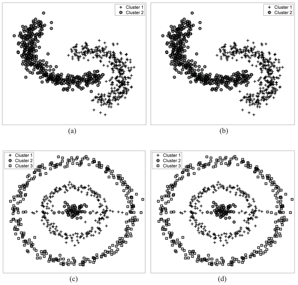
Figure 3. The clustering results obtained for the data with two bean-shaped clusters by (a) agglomerative clustering and (b) split and merge clustering. The clustering results obtained for the data with three concentric circle-shaped clusters by (c) agglomerative clustering and (d) split and merge clustering.

Figure 3. The clustering results obtained for the data with two bean-shaped clusters by (a) agglomerative clustering and (b) split and merge clustering. The clustering results obtained for the data with three concentric circle-shaped clusters by (c) agglomerative clustering and (d) split and merge clustering.

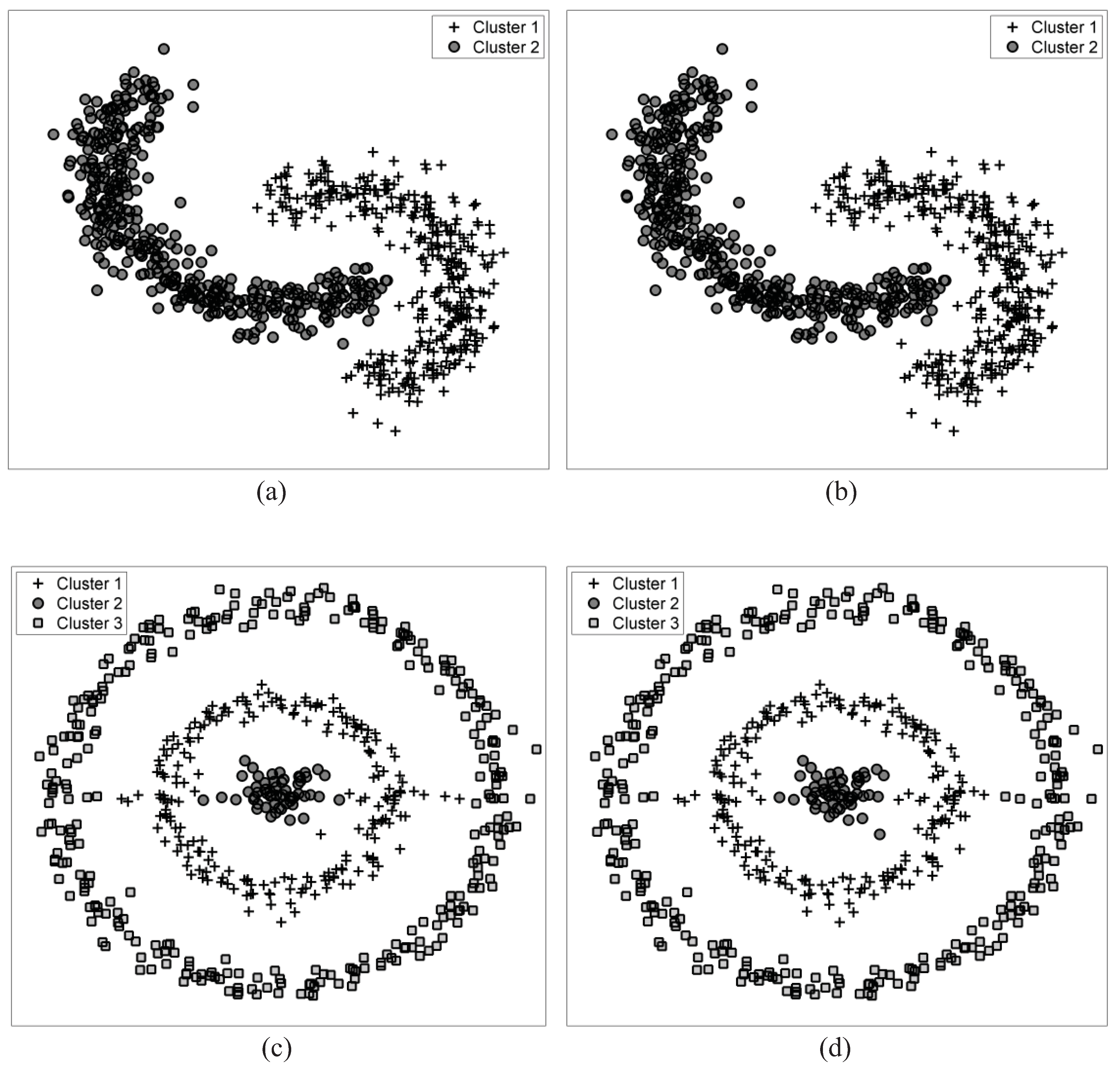
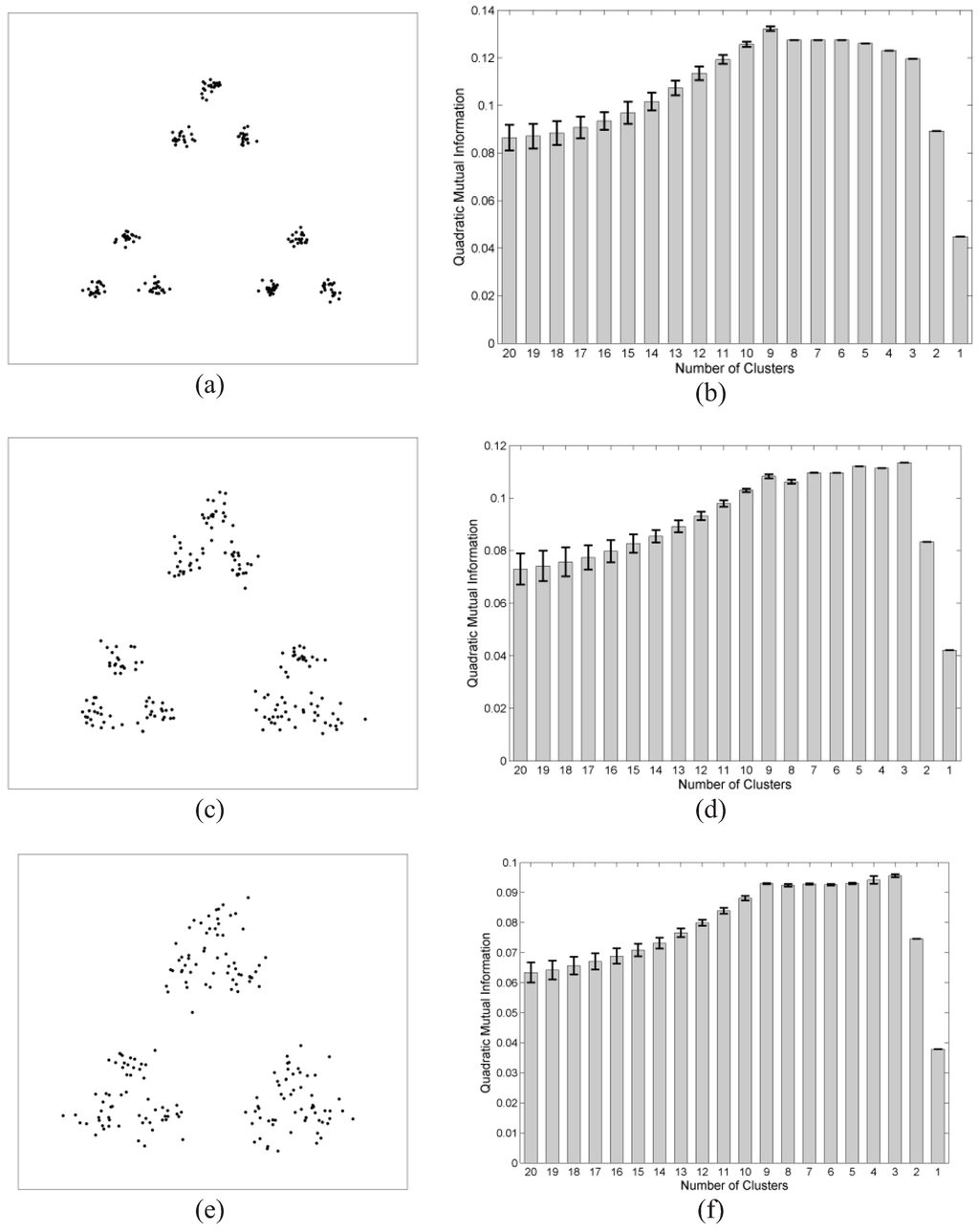
Figure 4. Data with 9 Gaussian distributed clusters arranged in three groups with variances (a) 0.02, (c) 0.04, and (e) 0.06. The mean quadratic mutual information and its standard deviation measured at each step of the split and merge clustering for ten trials is demonstrated. A clear global maximum at nine clusters is observed for (b). Subplots (d) and (f) show a local maximum at nine clusters and a global maximum at three, demonstrating the confusion in selecting nine clusters out of three group of clusters when the variance is relatively high.

Figure 4. Data with 9 Gaussian distributed clusters arranged in three groups with variances (a) 0.02, (c) 0.04, and (e) 0.06. The mean quadratic mutual information and its standard deviation measured at each step of the split and merge clustering for ten trials is demonstrated. A clear global maximum at nine clusters is observed for (b). Subplots (d) and (f) show a local maximum at nine clusters and a global maximum at three, demonstrating the confusion in selecting nine clusters out of three group of clusters when the variance is relatively high.

4. Conclusions

In this paper, mutual information has been used as an information theoretic proximity measure for clustering. Although information theoretic measures facilitate extracting data structures further than the second order statistics, but are challenged by the practical difficulties in estimating the distribution of samples in each cluster. We use the non-parametric Parzen window estimator with Gaussian kernels to estimate this distribution, where it has been shown to simplify the quadratic approximation of the mutual information into a sum of pairwise distances. Since the quadratic mutual information can be updated iteratively for newly generated clusters, it is an appropriate proximity measure for hierarchical clustering algorithms.

Two hierarchical approaches are proposed for maximizing the quadratic mutual information between the samples of the input space and the clusters, namely the agglomerative and the split and merge clustering. We demonstrated how maximizing the mutual information is analogous to optimizing the distortion-rate function that achieves the minimum distortion among samples of each clusters for a given rate, and therefore provides the best clustering result. Beginning from a preliminary set of clusters generated by the initial clustering, the agglomerative clustering finds the best pair of clusters to be merged at each step of the hierarchy, while the split and merge clustering eliminates the cluster with the worst effect on the mutual information, and reassigns its samples to the remaining clusters. Finally, the true number of clusters in the data is determined based on the rate of changes in the quadratic mutual information from different hierarchies. Although the split and merge clustering is computationally more expensive than the agglomerative clustering, it benefits from being less sensitive to the initial clustering and the selection of the variance for the Gaussian kernels.

Experimental results on both artificial and real datasets have illustrated the promising performance of our proposed algorithms, both in finding the nonlinear boundaries between complex-shape clusters and determining the true number of clusters in the data. While conventional clustering algorithms typically fail in detecting the true data structures of the introduced artificial datasets, the proposed algorithms were able to detect clusters with different shapes and sizes. The superiority of the proposed algorithms for real applications is demonstrated by their clustering performance on the Iris and Wine datasets in comparison with some clustering algorithms reported in the literature.

References

- Mahalanobis, P.C. On the generalized distance in statistics. Proc. Natl. Inst. Sci. India 1936, 12, 49–55. [Google Scholar]
- Hartigan, J.A.; Wong, M.A. A k-means clustering algorithm. JR Stat. Soc. Ser. C-Appl. Stat. 1979, 28, 100–108. [Google Scholar]
- Bezdek, J.C.; Ehrlich, R. FCM: The fuzzy c-means clustering algorithm. Comput. Geosci. 1984, 10, 191–203. [Google Scholar] [CrossRef]
- Johnson, S.C. Hierarchical clustering schemes. Psychometrika 1967, 32, 241–254. [Google Scholar] [CrossRef] [PubMed]
- Jain, A.K.; Mao, J.; Mohiuddin, K.M. Artificial neural networks: A tutorial. Computer 1996, 29, 31–44. [Google Scholar] [CrossRef]
- Cristianini, N.; Shawe-Taylor, J. An Introduction to Support Vector Machines: and Other Kernel-based Learning Methods; Cambridge University Press: Cambridge, UK, 2000. [Google Scholar]
- Davis, J.V.; Kulis, B.; Jain, P.; Sra, S.; Dhillon, I.S. Information-theoretic metric learning. In Proceedings of the 24th international conference on Machine learning (ICML ’07), New York, NY, USA; 2007; pp. 209–216. [Google Scholar]
- Chaudhuri, K.; McGregor, A. Finding metric structure in information theoretic clustering. In Conference on Learning Theory, COLT, Helsinki, Finland, July 2008.
- Roweis, S.; Ghahramani, Z. A unifying review of linear Gaussian models. Neural Comput. 1999, 11, 305–345. [Google Scholar] [CrossRef] [PubMed]
- Parzen, E. On estimation of a probability density function and mode. Ann. Math. Statist. 1962, 33, 1065–1076. [Google Scholar] [CrossRef]
- Kraskov, A.; Grassberger, P. MIC: mutual information based hierarchical clustering. In Information Theory Statistical Learning; Springer: New York, NY, USA, 2008; pp. 101–123. [Google Scholar]
- Zhou, X.; Wang, X.; Dougherty, E.R.; Russ, D.; Suh, E. Gene clustering based on clusterwide mutual information. J. Comput. Biol. 2004, 11, 147–161. [Google Scholar] [CrossRef] [PubMed]
- Rényi, V. On measures of information and entropy. In Proceedings of the 4th Berkeley Symposium on Mathematics, Statistics and Probability, Berkeley: University of California Press, California, USA; 1961; pp. 547–561. [Google Scholar]
- Principe, J.C.; Xu, D.; Fisher, J. Information theoretic learning. In Unsupervised Adaptive Filtering; Haykin, S., Ed.; Wiley: New York, NY, USA, 2000; pp. 265–319. [Google Scholar]
- Gokcay, E.; Principe, J.C. Information theoretic clustering. IEEE Trans. Patt. Anal. Mach. Int. 2002, 24, 158–171. [Google Scholar] [CrossRef]
- Torkkola, K. Feature extraction by non parametric mutual information maximization. J. Mach. Learn. Res. 2003, 3, 1438. [Google Scholar]
- Sullivan, G.J.; Wiegand, T. Rate-distortion optimization for video compression. Signal Process. Mag. IEEE 2002, 15, 74–90. [Google Scholar] [CrossRef]
- Shannon, C.E. A mathematical theory of communication. Bell Syst. Tech. J. 1948, 27, 379–423. [Google Scholar] [CrossRef]
- Cover, T.M.; Thomas, J.A. Elements of Information Theory, 2nd ed.; Wiley: New York, NY, USA, 2006. [Google Scholar]
- Kapur, J.N. Measures of Information and Their Applications; Wiley: New Delhi, India, 1994. [Google Scholar]
- Vincent, P.; Bengio, Y. Manifold parzen windows. Adv. Neural Inf. Process. Syst. 2003, 15, 849–856. [Google Scholar]
- Davis, J.V.; Dhillon, I. Differential entropic clustering of multivariate gaussians. Adv. Neural Inf. Process. Syst. 2007, 19, 337. [Google Scholar]
- Karypis, G.; Han, E.H.; Kumar, V. Chameleon: Hierarchical clustering using dynamic modeling. Computer 1999, 32, 68–75. [Google Scholar] [CrossRef]
- Guha, S.; Rastogi, R.; Shim, K. Cure: An efficient clustering algorithm for large databases. Inf. Syst. 2001, 26, 35–58. [Google Scholar] [CrossRef]
- Duda, R.O.; Hart, P.E. Pattern classification and scene analysis. Wiley, New York, NY, USA, 1973. [Google Scholar]
- Silverman, B.W. Density Estimation for Statistics and Data Analysis; Chapman & Hall/CRC: London, England, UK, 1998. [Google Scholar]
- Anderson, E. The irises of the Gaspe Peninsula. Bull. Am. IRIS Soc. 1935, 59, 2–5. [Google Scholar]
- Blatt, M.; Wiseman, S.; Domany, E. Superparamagnetic clustering of data. Phys. Rev. Lett. 1996, 76, 3251–3254. [Google Scholar] [CrossRef] [PubMed]
- Jenssen, R.; Erdogmus, D.; Ii, K.; Principe, J.; Eltoft, T. Information force clustering using directed trees. Lect. Note. Comput. Sci. 2003, 2683, 68–72. [Google Scholar]
- Aeberhard, S.; Coomans, D.; De Vel, O. Comparison of classifiers in high dimensional settings. Tech. Rep. 1992, 92–102. [Google Scholar]
- Sugar, C.A.; James, G.M. Finding the number of clusters in a dataset. J. Am. Statist. Assn. 2003, 98, 750–763. [Google Scholar] [CrossRef]
- Jenssen, R.; Hild, K.E.; Erdogmus, D.; Principe, J.C.; Eltoft, T. Clustering using Renyi’s entropy. Neural Networks 2003, 1, 523–528. [Google Scholar]
Appendix
Here we provide a proof for (15). The proof for each term, out of the three quadratic terms in (11), is presented separately. Starting from the first term we have:
Similarly, for the second term we have:
Finally, for the third term we have:
© 2011 by the authors; licensee MDPI, Basel, Switzerland. This article is an open access article distributed under the terms and conditions of the Creative Commons Attribution license (http://creativecommons.org/licenses/by/3.0/).