Eigenvalue Estimates Using the Kolmogorov-Sinai Entropy

Abstract

The scope of this paper is twofold. First, we use the Kolmogorov-Sinai Entropy to estimate lower bounds for dominant eigenvalues of nonnegative matrices. The lower bound is better than the Rayleigh quotient. Second, we use this estimate to give a nontrivial lower bound for the gaps of dominant eigenvalues of $\mathbf{A}$ and $\mathbf{A}+\mathbf{V}$.

1. Introduction

The main concern of this paper is to relate eigenvalue estimates to the Kolmogorov-Sinai entropy for Markov shifts. We shall begin with the definition of the Kolmogorov-Sinai entropy. Let $\mathbf{A}=\left(a_{ij}\right)\in {\mathbb{R}}^{N\times N}$ be an irreducible nonnegative matrix. By an irreducible matrix $\mathbf{A}$, we mean for each $1\le i,j\le N$, there exists positive integer k such that ${\left({\mathbf{A}}^k\right)}_{ij}\ne 0$. A matrix $\mathbf{P}=\left(p_{ij}\right)\in {\mathbb{R}}^{N\times N}$ is said to be a stochastic matrix compatible with $\mathbf{A}$, if $\mathbf{P}$ satisfies

• $0<p_{ij}\le 1$ if $a_{ij}>0$,
• $p_{ij}=0$ if $a_{ij}=0$,
• ${\displaystyle \sum _{j=1}^N{p}_{ij}=1}$, for all $i=1,\dots ,N$.

We denote by ${\mathcal{P}}_{\mathbf{A}}$ the set of all stochastic matrices compatible with $\mathbf{A}$. By Perron-Frobenius Theorem, it is easily seen that every stochastic matrix $\mathbf{P}$ has a unique left eigenvector $\mathbf{q}>0$ corresponding to eigenvalue 1 with ${\sum }_{i=1}^N{q}_i=1$. Here we say $\mathbf{q}$ is the stationary probability vector associated with $\mathbf{P}$. For a transition matrix $\mathbf{A}$, i.e., $a_{ij}=1$ or 0 for each $1\le i,j\le N$, the subshift of finite type generated by $\mathbf{A}$ is defined by

$$\begin{array}{c}\hfill {\Sigma }_{\mathbf{A}}=\{\mathbf{i}=(i_0,i_1,\dots )|i_j\in \{1,\dots ,N\},a_{i_j,i_{j+1}}=1,j=0,1,2,\dots \}\end{array}$$

and the shift map on ${\Sigma }_{\mathbf{A}}$ is defined by ${\sigma }_{\mathbf{A}}(i_0,i_1,\dots )=(i_1,i_2,\dots )$. A cylinder of ${\Sigma }_{\mathbf{A}}$ is the set

$$\begin{array}{c}\hfill C_{j_0,j_1,\dots ,j_n}=\{\mathbf{i}\in {\Sigma }_{\mathbf{A}}|i_0=j_0,\dots ,i_n=j_n\}\end{array}$$

for any $n\ge 0$. Disjoint unions of cylinders form an algebra which generates the Borel σ-algebra of ${\Sigma }_{\mathbf{A}}$. For any $\mathbf{P}\in {\mathcal{P}}_{\mathbf{A}}$ and its associated stationary probability vector $\mathbf{q}$, the Markov measure of a cylinder may then be defined by

$$\begin{array}{c}\hfill {\mu }_{\mathbf{P},\mathbf{q}}\left(C_{j_0,j_1,\dots ,j_n}\right)=q_{j_0}{p}_{j_0,j_1}\cdots p_{j_{n-1},j_n}\end{array}$$

Here ${\mu }_{\mathbf{P},\mathbf{q}}$ is an invariant measure under the shift map ${\sigma }_{\mathbf{A}}$ (see e.g., [8]). The Kolmogorov-Sinai entropy (or called the measure theoretic entropy) of ${\sigma }_{\mathbf{A}}$ under the invariant measure ${\mu }_{\mathbf{P},\mathbf{q}}$ is defined by

$$\begin{array}{c}\hfill h_{\mathbf{P},\mathbf{q}}\left({\sigma }_{\mathbf{A}}\right)=\underset{n\to \infty }{lim}\frac{1}{n}\sum _{j_0,j_1,\dots ,j_n}H\left({\mu }_{\mathbf{P},\mathbf{q}}\left(C_{j_0,j_1,\dots ,j_n}\right)\right)\end{array}$$

where $H\left(x\right)=-xlogx$ and the convention $0log0=0$ is adopted. The notion of the Kolmogorov-Sinai entropy was first studied by Kolmogorov in 1958 on the problems arising from information theory and dimension of functional spaces, that measures the uncertainty of the dynamical systems (see e.g., [6,7]). It is shown in [8] (p. 221) that

$$\begin{array}{c}\hfill h_{\mathbf{P},\mathbf{q}}\left({\sigma }_{\mathbf{A}}\right)=-\sum _{ij}{q}_i{p}_{ij}log{p}_{ij}\end{array}$$

(1)

where the summation in (1) is taken over all $i,j$ with $a_{ij}=1$. On the other hand, it is shown by Parry [9] (Theorems 6 and 7) that the Kolmogorov-Sinai entropy of ${\sigma }_{\mathbf{A}}$ has an upper bound $log{\lambda }_N\left(\mathbf{A}\right)$.

Theorem 1.1 (Parry’s Theorem).

Let $\mathbf{A}$ be an $N\times N$ irreducible transition matrix. Then for any $\mathbf{P}\in {\mathcal{P}}_{\mathbf{A}}$ and its associated stationary probability vector $\mathbf{q}$, we have

$$\begin{array}{c}\hfill h_{\mathbf{P},\mathbf{q}}\left({\sigma }_{\mathbf{A}}\right)\le log{\lambda }_N\left(\mathbf{A}\right)\end{array}$$

(2)

where ${\lambda }_N\left(\mathbf{A}\right)$ denotes the dominant eigenvalue of $\mathbf{A}$. Moreover, if $\mathbf{A}$ is regular (${\mathbf{A}}^n>0$ for some $n>0$), the equality in (2) holds for some unique $\mathbf{P}\in {\mathcal{P}}_{\mathbf{A}}$ and $\mathbf{q}$ the stationary probability vector associated with $\mathbf{P}$.

Parry’s Theorem shows the Kolmogorov-Sinai entropy for a Markov shift is less than or equal to its topological entropy (that is, $log{\lambda }_N\left(\mathbf{A}\right)$) and exactly one of the Markov measures on ${\Sigma }_{\mathbf{A}}$ maximizes the Kolmogorov-Sinai entropy of ${\sigma }_{\mathbf{A}}$ provided it is topological mixing. This is also a crucial lemma for showing the Variational Property of Entropy [8] (Proposition 8.1) in the ergodic theory. However, from the viewpoint of eigenvalue problems, combination of (1) and (2) gives a lower bound for the dominant eigenvalue of the transition matrix $\mathbf{A}$. In this paper, we generalize Parry’s Theorem to general $N\times N$ irreducible nonnegative matrices. Toward this end, we extend the entropy of irreducible nonnegative matrices by

$$h_{\mathbf{P},\mathbf{q},\mathbf{A}}=-\sum _{ij}{q}_i{p}_{ij}log\frac{p_{ij}}{a_{ij}}$$

It is easily seen that $h_{\mathbf{P},\mathbf{q},\mathbf{A}}=h_{\mathbf{P},\mathbf{q}}\left({\sigma }_{\mathbf{A}}\right)$.

Theorem 1.2 (Main Result 1: The Generalized Parry’s Theorem).

Let $\mathbf{A}\in {\mathbb{R}}^{N\times N}$ an irreducible nonnegative matrix. Let $\mathbf{P}\in {\mathcal{P}}_{\mathbf{A}}$ and $\mathbf{q}$ be a stationary probability vector associated with $\mathbf{P}$, then we have

$$\begin{array}{c}\hfill h_{\mathbf{P},\mathbf{q},\mathbf{A}}\le log{\lambda }_N\left(\mathbf{A}\right)\end{array}$$

(3)

where the summation is taken over all $i,j$ with $a_{ij}>0$. Moreover, the equality in (3) holds when

$$\begin{array}{c}\hfill \mathbf{P}=\frac{1}{{\lambda }_N\left(\mathbf{A}\right)}\mathrm{diag}{\left(\mathbf{x}\right)}^{-1}\mathbf{A}\mathrm{diag}\left(\mathbf{x}\right)\end{array}$$

and

$$\begin{array}{c}\hfill \mathbf{q}=\frac{\mathbf{y}\circ \mathbf{x}}{{\mathbf{y}}^{\top }\mathbf{x}}\end{array}$$

where $\mathbf{x}>0$ and $\mathbf{y}>0$ are, respectively, the right and left eigenvectors of $\mathbf{A}$ corresponding to the eigenvalue ${\lambda }_N\left(\mathbf{A}\right)$. Here, $\text{diag}\left(\mathbf{x}\right)$ denotes the diagonal matrix with $\mathbf{x}$ on its diagonal, $\mathbf{y}\circ \mathbf{x}$ denotes the vector $(y_1{x}_1,\dots ,y_N{x}_N)$, and ${\mathbf{y}}^{\top }$ denotes the transpose of the column vector $\mathbf{y}$.

Lower bound estimates for the dominant eigenvalue of a symmetric irreducible nonnegative matrix play an important role in various fields, e.g., the complexity of a symbolic dynamical system [5], synchronization problem of coupled systems [10], or the ground state estimates of Schrödinger operators [2]. A usual way to estimate the lower bound for ${\lambda }_N\left(\mathbf{A}\right)$ is the Rayleigh quotient

$${\lambda }_N\left(\mathbf{A}\right)\ge \frac{{\mathbf{x}}^{\top }\mathbf{A}\mathbf{x}}{{\mathbf{x}}^{\top }\mathbf{x}}$$

It is also well-known that (see e.g., [4] (Theorem 8.1.26)),

$$\begin{array}{c}\hfill \underset{1\le i\le N}{min}\frac{1}{x_i}\sum _{j=1}^N{a}_{ij}{x}_j\le {\lambda }_N\left(\mathbf{A}\right)\le \underset{1\le i\le N}{max}\frac{1}{x_i}\sum _{j=1}^N{a}_{ij}{x}_j\end{array}$$

(4)

provided that $\mathbf{A}\in {\mathbb{R}}^{N\times N}$ is nonnegative and $\mathbf{x}\in {\mathbb{R}}^N$ is positive. Comparing the lower bound estimate (3) with (4) as well as with the Rayleigh quotient, we have the following result.

Corollary 1.3.

Let $\mathbf{A}\in {\mathbb{R}}^{N\times N}$ be a symmetric, irreducible nonnegative matrix. Suppose $\mathbf{x}\in {\mathbb{R}}^N$ be positive. Then the matrix ${\displaystyle \mathbf{P}=\mathrm{diag}{\left(\mathbf{A}\mathbf{x}\right)}^{-1}\mathbf{A}\mathrm{diag}\left(\mathbf{x}\right)}$ is in ${\mathcal{P}}_{\mathbf{A}}$ and ${\displaystyle \mathbf{q}=\frac{\mathbf{x}\circ \left(\mathbf{A}\mathbf{x}\right)}{{\mathbf{x}}^{\top }\mathbf{A}\mathbf{x}}}$ is the stationary probability vector associated with $\mathbf{P}$. In addition,

$$\begin{array}{c}\hfill h_{\mathbf{P},\mathbf{q},\mathbf{A}}\ge log\left(\underset{1\le i\le N}{min}\frac{1}{x_i}\sum _{j=1}^N{a}_{ij}{x}_j\right)\end{array}$$

and

$$\begin{array}{c}\hfill h_{\mathbf{P},\mathbf{q},\mathbf{A}}\ge log\left(\frac{{\mathbf{x}}^{\top }\mathbf{A}\mathbf{x}}{{\mathbf{x}}^{\top }\mathbf{x}}\right)\end{array}$$

Here, each equality holds if and only if $\mathbf{x}$ is the eigenvector of $\mathbf{A}$ corresponding to the eigenvalue ${\lambda }_N\left(\mathbf{A}\right)$.

Here we remark that for any arbitrary irreducible nonnegative matrix $\mathbf{A}$, the entropy $h_{\mathbf{P},\mathbf{q},\mathbf{A}}$ involves the left eigenvector $\mathbf{q}$ of $\mathbf{P}$. Hence, the lower bound estimate (3) is merely a formal expression. However, for a symmetric irreducible nonnegative matrix $\mathbf{A}$ and $\mathbf{P}$ chosen as in Corollary 1.3, the vector $\mathbf{q}$ can be explicitly expressed. Therefore, $h_{\mathbf{P},\mathbf{q},\mathbf{A}}$ can be written in an explicit form. We shall further show in Proposition 2.6 that $h_{\mathbf{P},\mathbf{q},\mathbf{A}}=\frac{-1}{{\mathbf{x}}^{\top }\mathbf{y}}{\sum }_{i=1}^N{x}_i{y}_{i}log\frac{x_i}{y_i}$ where $\mathbf{y}=\mathbf{A}\mathbf{x}$.

Considering symmetric nonnegative $\mathbf{A}$ and its perturbation $\mathbf{A}+\mathbf{V}$, it is easily seen that ${\lambda }_N(\mathbf{A}+\mathbf{V})-{\lambda }_N\left(\mathbf{A}\right)\ge {\mathbf{x}}^{\top }\mathbf{V}\mathbf{x}$, where $\mathbf{x}$ is the normalized eigenvector of $\mathbf{A}$ corresponding to ${\lambda }_N\left(\mathbf{A}\right)$. This gives a trivial lower bound for the gap of ${\lambda }_N(\mathbf{A}+\mathbf{V})$ and ${\lambda }_N\left(\mathbf{A}\right)$. Upper bound estimates for the gap are well studied in the perturbation theory [4,11]. By considering $\mathbf{A}+\mathbf{V}$ as a low rank perturbation of $\mathbf{A}$, the interlace structure of eigenvalues of $\mathbf{A}+\mathbf{V}$ and of $\mathbf{A}$ is studied by [1,3]. In the second result of this paper, we give a nontrivial lower bound for ${\lambda }_N(\mathbf{A}+\mathbf{V})-{\lambda }_N\left(\mathbf{A}\right)$.

Theorem 1.4 (Main Result 2).

Let $\mathbf{A}\in {\mathbb{R}}^{N\times N}$ be an irreducible nonnegative matrix and $\mathbf{x}>0$ be the eigenvector of $\mathbf{A}$ corresponding to ${\lambda }_N\left(\mathbf{A}\right)$ with ${\parallel \mathbf{x}\parallel }_2=1$. Suppose $\mathbf{A}$ is symmetric. Then for any nonnegative $\mathbf{V}=\mathrm{diag}(v_1,\dots ,v_N)$, we have

$$\begin{array}{cc}\hfill {\lambda }_N(\mathbf{A}+\mathbf{V})-{\lambda }_N\left(\mathbf{A}\right)& \ge \frac{f(1/{\lambda }_N\left(\mathbf{A}\right))-1}{1/{\lambda }_N\left(\mathbf{A}\right)}\hfill \end{array}$$

(5)

where

$$\begin{array}{cc}\hfill f\left(z\right)& =\prod _{i=1}^N{(1+v_{i}z)}^{\frac{(1+v_{i}z)x_i^2}{{\sum }_{j=1}^N(1+v_{j}z)x_i^2}}\hfill \end{array}$$

Here $(f(1/{\lambda }_N\left(\mathbf{A}\right))-1){\lambda }_N\left(\mathbf{A}\right)\ge {\mathbf{x}}^{\top }\mathbf{V}\mathbf{x}$. Furthermore, the equality in (5) holds if and only if $v_1=\cdots =v_N$.

This paper is organized as follows. In Section 2, we prove the generalized Parry’s Theorem in three steps. First, we prove the case in which the matrix $\mathbf{A}$ has only integer entries. Next we show that Theorem 1.2 is true for nonnegative matrices with rational entries. Finally we show that it holds true for all irreducible nonnegative matrices. The proof of Corollary 1.3 is given at the end of this section. In Section 3, we give the proof of Theorem 1.4. We conclude this paper in Section 4.

Throughout this paper, we use the boldface alphabet (or symbols) to denote matrices (or vectors). For $\mathbf{u},\mathbf{v}\in {\mathbb{R}}^N$, the Hadamard product of $\mathbf{u}$ and $\mathbf{v}$ is their elementwise product which is denoted by $\mathbf{u}\circ \mathbf{v}={\left(u_i{v}_i\right)}_{1\le i\le N}$. The notation $\mathrm{diag}\left(\mathbf{u}\right)$ denotes the $N\times N$ diagonal matrix with $\mathbf{u}$ on its diagonal. A matrix $\mathbf{A}=\left(a_{ij}\right)\in {\mathbb{R}}^{N\times N}$ is said to be a transition matrix if $a_{ij}=1$ or 0 for all $1\le i,j\le N$. ${\lambda }_1\left(\mathbf{A}\right)\le \cdots \le {\lambda }_N\left(\mathbf{A}\right)$ denotes the dominant eigenvalue of a nonnegative matrix $\mathbf{A}$.

2. Proof of the Generalized Parry’s Theorem and Corollary 1.3

In this section, we shall prove the generalized Parry’s Theorem and Corollary 1.3. To prove inequality (3), we proceed in three steps.

Step 1: Inequality (3) is true for all irreducible nonnegative matrices with integer entries.

Let $\mathbf{A}$ be an irreducible nonnegative matrix with integer entries. To adopt Parry’s Theorem, we shall construct a transition matrix $\overline{\mathbf{A}}$ corresponding to $\mathbf{A}$ for which ${\lambda }_N\left(\overline{\mathbf{A}}\right)={\lambda }_N{\left(\mathbf{A}\right)}^{1/2}$. To this end, we define the sets of indexes:

$$\begin{array}{cc}\hfill \mathcal{I}& =\{1,\dots ,N\}\hfill \\ \hfill \mathcal{E}& =\left\{{\overrightarrow{ij}}^{\left(k\right)}\right|a_{ij}\ne 0,1\le k\le a_{ij}\}\hfill \end{array}$$

Let $\tilde{N}={\sum }_{i,j=1}^N{a}_{ij}=\#\mathcal{E}$ and $\overline{N}=N+\tilde{N}$. The transition matrix $\overline{\mathbf{A}}\in {\mathbb{R}}^{\overline{N}\times \overline{N}}$ corresponding to $\mathbf{A}$ with index set $\mathcal{I}\cup \mathcal{E}$ is defined as follows

$$\begin{array}{cc}& \text{(1)}{\overline{a}}_{i,{\overrightarrow{ij}}^{\left(k\right)}}=1,\text{for}\text{all}1\le k\le a_{ij}\text{if}{a}_{ij}\ne 0,\hfill \end{array}$$

(6a)

$$\begin{array}{cc}& \text{(2)}{\overline{a}}_{{\overrightarrow{ij}}^{\left(k\right)},j}=1,\text{for}\text{all}1\le k\le a_{ij}\text{if}{a}_{ij}\ne 0,\hfill \end{array}$$

(6b)

$$\begin{array}{cc}& \text{(3)}\text{the}\text{rest}\text{entries}\text{are}\text{set}\text{to}\text{be}\text{zero}\hfill \end{array}$$

(6c)

It is easily seen that $\overline{\mathbf{A}}$ can be written in the block form:

$$\begin{array}{c}\hfill \overline{\mathbf{A}}=\left[\begin{array}{cc}{0}_{N\times N}& {\overline{\mathbf{A}}}_{\mathcal{I}\mathcal{E}}\\ {\overline{\mathbf{A}}}_{\mathcal{E}\mathcal{I}}& 0_{\tilde{N}\times \tilde{N}}\end{array}\right]\end{array}$$

(7)

where $0_{N\times N}$ and $0_{\tilde{N}\times \tilde{N}}$ are, respectively, the zero matrices in ${\mathbb{R}}^{N\times N}$ and ${\mathbb{R}}^{\tilde{N}\times \tilde{N}}$, ${\overline{\mathbf{A}}}_{\mathcal{I}\mathcal{E}}\in {\mathbb{R}}^{N\times \tilde{N}}$ and ${\overline{\mathbf{A}}}_{\mathcal{E}\mathcal{I}}\in {\mathbb{R}}^{\tilde{N}\times N}$.

Proposition 2.1.

${\lambda }_{\overline{N}}\left(\overline{\mathbf{A}}\right)={\lambda }_N{\left(\mathbf{A}\right)}^{1/2}$.

Proof.

From (7), we see that

$$\begin{array}{c}\hfill {\overline{\mathbf{A}}}^2=\left[\begin{array}{cc}{\overline{\mathbf{A}}}_{\mathcal{I}\mathcal{E}}{\overline{\mathbf{A}}}_{\mathcal{E}\mathcal{I}}& 0_{N\times \tilde{N}}\\ 0_{\tilde{N}\times N}& {\overline{\mathbf{A}}}_{\mathcal{E}\mathcal{I}}{\overline{\mathbf{A}}}_{\mathcal{I}\mathcal{E}}\end{array}\right]\end{array}$$

From (6a) and (6b), for each $i,j$ with $a_{ij}\ne 0$, we have

$$\begin{array}{c}\hfill \sum _{k=1}^{a_{ij}}{\overline{a}}_{i,{\overrightarrow{ij}}^{\left(k\right)}}{\overline{a}}_{{\overrightarrow{ij}}^{\left(k\right)},j}=a_{ij}\end{array}$$

(8)

Using (8), together with (6c), we have

$$\begin{array}{cc}\hfill {\left({\overline{\mathbf{A}}}_{\mathcal{I}\mathcal{E}}{\overline{\mathbf{A}}}_{\mathcal{E}\mathcal{I}}\right)}_{ij}& =\sum _{\alpha \in \mathcal{E}}{\overline{a}}_{i\alpha }{\overline{a}}_{\alpha j}\hfill \end{array}$$

$$\begin{array}{cc}& =\left\{\begin{array}{cc}\sum _k{\overline{a}}_{i,{\overrightarrow{ij}}^{\left(k\right)}}{\overline{a}}_{{\overrightarrow{ij}}^{\left(k\right)},j}=a_{ij}\hfill & \text{if}{a}_{ij}\ne 0\hfill \\ 0=a_{ij}\hfill & \text{if}{a}_{ij}=0\hfill \end{array}\right.\hfill \end{array}$$

(9)

From (9) we see that ${\overline{\mathbf{A}}}_{\mathcal{I}\mathcal{E}}{\overline{\mathbf{A}}}_{\mathcal{E}\mathcal{I}}=\mathbf{A}$. Hence ${\lambda }_{\overline{N}}\left({\overline{\mathbf{A}}}^2\right)={\lambda }_N\left({\overline{\mathbf{A}}}_{\mathcal{I}\mathcal{E}}{\overline{\mathbf{A}}}_{\mathcal{E}\mathcal{I}}\right)={\lambda }_{\tilde{N}}\left({\overline{\mathbf{A}}}_{\mathcal{E}\mathcal{I}}{\overline{\mathbf{A}}}_{\mathcal{I}\mathcal{E}}\right)={\lambda }_N\left(\mathbf{A}\right)$. On the other hand, $\overline{\mathbf{A}}$ is a nonnegative matrix. From Perron-Frobenius Theorem, its dominant eigenvalue is nonnegative. The assertion follows. ☐

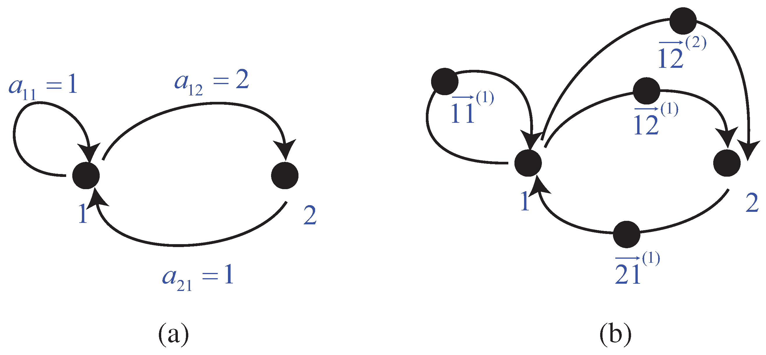
Remark 2.1. In the language of graph theory, $a_{ij}$ represents the number of directed edges from vertex i to vertex j. Hence ${\sum }_{ij}{\left({\mathbf{A}}^n\right)}_{ij}$ equals to the number of all possible routes of length $n+1$, i.e.,

$$\begin{array}{c}\hfill \#\left\{\text{all}\text{possible}\text{routes}\text{of}\text{length}n+1\right\}=\sum _{ij}{\left({\mathbf{A}}^n\right)}_{ij}=O\left({\lambda }_N{\left(\mathbf{A}\right)}^n\right)\end{array}$$

For the construction of $\overline{\mathbf{A}}$, we add an additional vertex on every edge from vertex i to vertex j (See Figure 2.1 for the illustration). Hence, each route that obeys the rule defined by $\mathbf{A}$,

$$\begin{array}{c}\hfill (i_1,i_2,\dots ,i_j,i_{j+1},\dots ,i_{n-1},i_n),\text{provided}{a}_{i_j{i}_{j+1}}>0\text{for}\text{all}j=1,\cdots ,n-1\end{array}$$

(10)

now becomes one of the following routes according to the rule defined by $\overline{\mathbf{A}}$:

$$\begin{array}{c}\hfill (i_1,{\overrightarrow{i_1{i}_2}}^{\left(k_1\right)},i_2,\dots i_j,{\overrightarrow{i_j{i}_{j+1}}}^{\left(k_j\right)}{i}_{j+1},\dots ,i_{n-1},{\overrightarrow{i_{n-1}{i}_n}}^{\left(k_{n-1}\right)},i_n)\end{array}$$

(11)

where $1\le k_j\le a_{i_j{i}_{j+1}}$, $j=1,\dots ,n-1$. However, a route of the form in (11) is equivalent to the form in (10) but its length is doubled. Hence $O\left({\lambda }_N{\left(\overline{\mathbf{A}}\right)}^{2n}\right)=O\left({\lambda }_N{\left(\mathbf{A}\right)}^n\right)$.

Figure 1. Illustration for Remark 2.1 with the example $\mathbf{A}=\left[\begin{array}{cc}1& 2\\ 1& 0\end{array}\right]$.

Now, let $\mathbf{P}\in {\mathcal{P}}_{\mathbf{A}}$ be given and $\mathbf{q}$ be its associated stationary probability vector. We shall accordingly define a stochastic matrix $\overline{\mathbf{P}}\in {\mathcal{P}}_{\overline{\mathbf{A}}}$ and its associated stationary probability vector $\overline{\mathbf{q}}$. The stochastic matrix $\overline{\mathbf{P}}$ is defined as follows:

$$\begin{array}{cc}& \text{(1)}{\overline{p}}_{i,{\overrightarrow{ij}}^{\left(k\right)}}=\frac{p_{ij}}{a_{ij}}\text{for}\text{all}1\le k\le a_{ij}\text{provided}{a}_{ij}>0\hfill \end{array}$$

(12a)

$$\begin{array}{cc}& \text{(2)}{\overline{p}}_{{\overrightarrow{ij}}^{\left(k\right)},j}=1\text{for}\text{all}1\le k\le a_{ij}\text{provided}{a}_{ij}>0\hfill \end{array}$$

(12b)

$$\begin{array}{cc}& \text{(3)}\text{the}\text{rest}\text{entries}\text{are}\text{set}\text{to}\text{zero}\hfill \end{array}$$

(12c)

From (6) and (12), it is easily seen that $\overline{\mathbf{P}}$ is a stochastic matrix compatible with $\overline{\mathbf{A}}$. Let the vector $\overline{\mathbf{q}}\in {\mathbb{R}}^{N+\tilde{N}}$ be defined by

$$\begin{array}{c}\hfill {\overline{q}}_i=\frac{q_i}{2},1\le i\le N\end{array}$$

(13a)

and

$$\begin{array}{c}\hfill {\overline{q}}_{{\overrightarrow{ij}}^{\left(k\right)}}=\frac{q_i{p}_{ij}}{2a_{ij}},\text{for}\text{all}1\le k\le a_{ij}\text{with}{a}_{ij}>0\end{array}$$

(13b)

Proposition 2.2.

$\overline{\mathbf{q}}$ is the stationary probability vector associated with $\overline{\mathbf{P}}$.

Proof.

We first show that $\overline{\mathbf{q}}$ is a left eigenvector of $\overline{\mathbf{P}}$ with the corresponding eigenvalue 1. For any $1\le j\le N$, using (12b), (13b), and the fact that ${\mathbf{q}}^{\top }\mathbf{P}={\mathbf{q}}^{\top }$, we have

$$\begin{array}{cc}\hfill {\left({\overline{\mathbf{q}}}^{\top }\overline{\mathbf{P}}\right)}_j=\sum _{i,k}{\overline{q}}_{{\overrightarrow{ij}}^{\left(k\right)}}{\overline{p}}_{{\overrightarrow{ij}}^{\left(k\right)},j}& =\sum _{i,a_{ij}>0}\sum _{k=1}^{a_{ij}}\frac{1}{2}{q}_i\frac{p_{ij}}{a_{ij}}·1\hfill \end{array}$$

$$\begin{array}{cc}& =\sum _i\frac{1}{2}{q}_i{p}_{ij}=\frac{1}{2}{q}_j={\overline{q}}_j\hfill \end{array}$$

(14a)

On the other hand, using (12a) and (13a), for all ${\overrightarrow{ij}}^{\left(k\right)}$ with $a_{ij}>0$ and $1\le k\le a_{ij}$, we have

$$\begin{array}{cc}\hfill {\left({\overline{\mathbf{q}}}^{\top }\overline{\mathbf{P}}\right)}_{{\overrightarrow{ij}}^{\left(k\right)}}& ={\overline{q}}_i{\overline{p}}_{i,{\overrightarrow{ij}}^{\left(k\right)}}\hfill \end{array}$$

$$\begin{array}{cc}& =\frac{1}{2}{q}_i\frac{p_{ij}}{a_{ij}}={\overline{q}}_{{\overrightarrow{ij}}^{\left(k\right)}}\hfill \end{array}$$

(14b)

In (14), we have proved ${\overline{\mathbf{q}}}^{\top }\overline{\mathbf{P}}={\overline{\mathbf{q}}}^{\top }$. Now we show that the total sum of entries of $\overline{\mathbf{q}}$ is 1. Using the fact

$$\begin{array}{cc}\hfill \sum _{ij}\sum _{k=1}^{a_{ij}}{\overline{q}}_{{\overrightarrow{ij}}^{\left(k\right)}}& =\sum _{ij}\sum _{k=1}^{a_{ij}}\frac{q_i{p}_{ij}}{2a_{ij}}\hfill \\ & =\sum _{ij}\frac{1}{2}{q}_i{p}_{ij}=\frac{1}{2}\sum _i{q}_i\hfill \end{array}$$

we conclude that

$$\begin{array}{cc}\hfill \sum _{\alpha \in \mathcal{I}\cup \mathcal{E}}{\left(\mathbf{q}\right)}_{\alpha }& =\sum _i{\overline{q}}_i+\sum _{ij}\sum _{k=1}^{a_{ij}}{\overline{q}}_{{\overrightarrow{ij}}^{\left(k\right)}}\hfill \\ & =\frac{1}{2}\sum q_i+\frac{1}{2}\sum _i{q}_i=1\hfill \end{array}$$

The proof is complete. ☐

From the construction of the transition matrix $\overline{\mathbf{A}}$, it is easily seen that $\overline{\mathbf{A}}$ is irreducible. In (12) and Proposition 2.2, we show that $\overline{\mathbf{P}}\in {\mathcal{P}}_{\overline{\mathbf{A}}}$ and the vector $\overline{\mathbf{q}}$ defined by (13) is its associated stationary probability vector. Hence the Kolmogorov-Sinai entropy $h_{\overline{\mathbf{P}},\overline{\mathbf{q}}}\left({\sigma }_{\overline{\mathbf{A}}}\right)$ is well-defined. Now we give the relationship between the quantities $h_{\overline{\mathbf{P}},\overline{\mathbf{q}}}\left({\sigma }_{\overline{\mathbf{A}}}\right)$ and $h_{\mathbf{P},\mathbf{q},\mathbf{A}}$ defined in Equation (3).

Proposition 2.3.

$$\begin{array}{c}\hfill h_{\overline{\mathbf{P}},\overline{\mathbf{q}}}\left({\sigma }_{\overline{\mathbf{A}}}\right)=\frac{1}{2}{h}_{\mathbf{P},\mathbf{q},\mathbf{A}}\end{array}$$

Proof.

We note that by (12b), $log{\overline{p}}_{{\overrightarrow{ij}}^{\left(k\right)},j}=0$ if $a_{ij}>0$. Using the definition of $\overline{\mathbf{P}}$ and $\overline{\mathbf{q}}$ in (12) and (13), as well as the entropy formula (1), we have

$$\begin{array}{cc}\hfill h_{\overline{\mathbf{P}},\overline{\mathbf{q}}}\left({\sigma }_{\overline{\mathbf{A}}}\right)& =-\sum _{ij,a_{ij}>0}\sum _{k=1}^{a_{ij}}{\overline{q}}_i{\overline{p}}_{i,{\overrightarrow{ij}}^{\left(k\right)}}log{\overline{p}}_{i,{\overrightarrow{ij}}^{\left(k\right)}}\hfill \\ & =-\sum _{ij,a_{ij}>0}\sum _{k=1}^{a_{ij}}\frac{1}{2}{q}_i\frac{p_{ij}}{a_{ij}}log\frac{p_{ij}}{a_{ij}}\hfill \\ & =-\sum _{ij,a_{ij}>0}\frac{1}{2}{q}_i{p}_{ij}log\frac{p_{ij}}{a_{ij}}\hfill \\ & =\frac{1}{2}{h}_{\mathbf{P},\mathbf{q},\mathbf{A}}\hfill \end{array}$$

The proof is complete. ☐

Using Proposition 2.3, 2.1, and Parry’s Theorem 1.1, it follows that

$$\begin{array}{cc}\hfill \frac{1}{2}{h}_{\mathbf{P},\mathbf{q},\mathbf{A}}& =h_{\overline{\mathbf{P}},\overline{\mathbf{q}}}\left({\sigma }_{\overline{\mathbf{A}}}\right)\hfill \end{array}$$

$$\begin{array}{cc}& \le log{\lambda }_N\left(\overline{\mathbf{A}}\right)=\frac{1}{2}log{\lambda }_N\left(\mathbf{A}\right)\hfill \end{array}$$

(15)

Step 2: Inequality (3) is true for all irreducible nonnegative matrices with rational entries.

Any $N\times N$ nonnegative matrix with all entries that are rational can be written as $\mathbf{A}/n$ where $\mathbf{A}$ is a nonnegative matrix with integer entries and n is an positive integer. Suppose $\mathbf{A}$ is irreducible and $\mathbf{P}\in {\mathcal{P}}_{\mathbf{A}/n}$. Note that ${\mathcal{P}}_{\mathbf{A}/n}={\mathcal{P}}_{\mathbf{A}}$. Letting $\mathbf{q}$ be a stationary probability vector associated with $\mathbf{P}$, inequality (3) for $\mathbf{A}/n$ follows from the following proposition.

Proposition 2.4.

$$\begin{array}{c}\hfill h_{\mathbf{P},\mathbf{q},\mathbf{A}/n}\le log{\lambda }_N(\mathbf{A}/n)\end{array}$$

Proof.

From the definition of $h_{\mathbf{P},\mathbf{q},\mathbf{A}/n}$, we see that

$$\begin{array}{cc}\hfill h_{\mathbf{P},\mathbf{q},\mathbf{A}/n}=-\sum _{ij,a_{ij}>0}{q}_i{p}_{ij}log\frac{p_{ij}n}{a_{ij}}& =-\sum _{ij,a_{ij}>0}{q}_i{p}_{ij}log\frac{p_{ij}}{a_{ij}}-\sum _{ij}{q}_i{p}_{ij}logn\hfill \end{array}$$

$$\begin{array}{cc}& =h_{\mathbf{P},\mathbf{q},\mathbf{A}}-\sum _{ij}{q}_i{p}_{ij}logn\hfill \end{array}$$

(16)

On the other hand, since ${\mathbf{q}}^{\top }\mathbf{P}={\mathbf{q}}^{\top }$ and $\sum q_i=1$, we have

$$\begin{array}{c}\hfill \sum _{ij}{q}_i{p}_{ij}logn=logn\end{array}$$

(17)

Substituting (17) into (16) and using the result (15) in Step 1, we have

$$\begin{array}{c}\hfill h_{\mathbf{P},\mathbf{q},\mathbf{A}/n}=h_{\mathbf{P},\mathbf{q},\mathbf{A}}-logn\le log{\lambda }_N\left(\mathbf{A}\right)-logn=log{\lambda }_N(\mathbf{A}/n)\end{array}$$

☐

Step 3: Inequality (3) is true for all irreducible nonnegative matrices.

It remains to show (3) holds for all nonnegative $\mathbf{A}$ with irrational entries. The assertion follows from Step 2 and the continuous dependence of eigenvalues with respect to the matrix.

Now, we give the proof of the second assertion of Theorem 1.2.

Proposition 2.5.

The equality in (3) holds when one chooses

$$\begin{array}{c}\hfill \mathbf{P}=\frac{1}{{\lambda }_N\left(\mathbf{A}\right)}\mathrm{diag}{\left(\mathbf{x}\right)}^{-1}\mathbf{A}\mathrm{diag}\left(\mathbf{x}\right)\end{array}$$

and

$$\begin{array}{c}\hfill \mathbf{q}=\frac{\mathbf{y}\circ \mathbf{x}}{{\mathbf{y}}^{\top }\mathbf{x}}\end{array}$$

where $\mathbf{x}>0$ and $\mathbf{y}>0$ are, respectively, the right and left eigenvectors of $\mathbf{A}$ corresponding to eigenvalue ${\lambda }_N\left(\mathbf{A}\right)$.

Proof.

By setting ${\mathbf{y}}^{\top }\mathbf{x}=1$, we may write

$$\begin{array}{c}\hfill p_{ij}=\frac{a_{ij}{x}_j}{{\lambda }_N\left(\mathbf{A}\right)x_i}\text{and}{q}_i=x_i{y}_i\end{array}$$

To ease the notation, set ${\lambda }_N={\lambda }_N\left(\mathbf{A}\right)$. Hence, we have

$$\begin{array}{cc}\hfill h_{\mathbf{P},\mathbf{q},\mathbf{A}}& =-\sum _{ij}{x}_i{y}_i\frac{a_{ij}{x}_j}{{\lambda }_N{x}_i}log\frac{x_j}{{\lambda }_N{x}_i}\hfill \\ & =\sum _{ij}\frac{y_i}{{\lambda }_N}\left(a_{ij}{x}_j\right)log\left({\lambda }_N{x}_i\right)-\sum _{ij}\frac{x_j}{{\lambda }_N}\left(y_i{a}_{ij}\right)log{x}_j\hfill \\ & =\sum _i{y}_i{x}_{i}log\left({\lambda }_N{x}_i\right)-\sum _j{x}_j{y}_{j}log{x}_j\left(\text{Use}\text{the}\text{facts}{\sum }_j{a}_{ij}{x}_j={\lambda }_N{x}_i\text{and}{\sum }_i{y}_i{a}_{ij}={\lambda }_N{y}_j\right)\hfill \\ & =\sum _i{x}_i{y}_{i}log{\lambda }_N\hfill \\ & =log{\lambda }_N\hfill \end{array}$$

The proof of Theorem 1.2 is complete. ☐

In the following, we give the proof of Corollary 1.3. We first prove the following useful proposition. It will be used in Section 3 as well.

Proposition 2.6.

Let $\mathbf{A}\in {\mathbb{R}}^{N\times N}$ be an irreducible nonnegative matrix. Suppose $\mathbf{A}$ is symmetric and $\mathbf{x}\in {\mathbb{R}}^N$ be positive. If $\mathbf{P}=\mathrm{diag}{\left(\mathbf{A}\mathbf{x}\right)}^{-1}\mathbf{A}\mathrm{diag}\left(\mathbf{x}\right)$ and $\mathbf{q}=\frac{\mathbf{x}\circ \mathbf{y}}{{\mathbf{x}}^{\top }\mathbf{y}}$, where $\mathbf{y}=\mathbf{A}\mathbf{x}$, then

$$\begin{array}{c}\hfill h_{\mathbf{P},\mathbf{q},\mathbf{A}}=\frac{-1}{{\mathbf{x}}^{\top }\mathbf{y}}\sum _{i=1}^N{x}_i{y}_{i}log\frac{x_i}{y_i}\end{array}$$

From Proposition 2.5, we see that the matrix $\mathbf{P}$ in Proposition 2.5 is a stochastic matrix compatible with $\mathbf{A}$ and $\mathbf{q}$ is its associated stationary probability vector. Hence, the entropy $h_{\mathbf{P},\mathbf{q},\mathbf{A}}$ is well defined. Now, we give the proof of this Proposition.

Proof. Since $\mathbf{A}\ge 0$ is irreducible and $\mathbf{x}>0$, it follows $\mathbf{A}\mathbf{x}>0$, and hence, $\mathrm{diag}{\left(\mathbf{A}\mathbf{x}\right)}^{-1}$ is well-defined. It is easily seen that $p_{ij}=0$ if and only if $a_{ij}=0$. However, $\mathbf{P}\mathbf{e}=\mathrm{diag}{\left(\mathbf{A}\mathbf{x}\right)}^{-1}\left(\mathbf{A}\mathbf{x}\right)=\mathbf{e}$. This shows that $\mathbf{P}\in {\mathcal{P}}_{\mathbf{A}}$. On the other hand, since $\mathbf{A}$ is symmetric, we see that ${\mathbf{y}}^{\top }={\mathbf{x}}^{\top }\mathbf{A}$. Hence

$$\begin{array}{c}\hfill {\mathbf{q}}^{\top }\mathbf{P}={(\mathbf{x}\circ \left(\mathbf{A}\mathbf{x}\right))}^{\top }\mathrm{diag}{\left(\mathbf{A}\mathbf{x}\right)}^{-1}\mathbf{A}\mathrm{diag}\left(\mathbf{x}\right)/{\mathbf{x}}^{\top }\mathbf{A}\mathbf{x}={\mathbf{q}}^{\top }\end{array}$$

We have proved the first assertion of this proposition. By the definition of $h_{\mathbf{P},\mathbf{q},\mathbf{A}}$ in (3), we have

$$\begin{array}{cc}\hfill h_{\mathbf{P},\mathbf{q},\mathbf{A}}& =-\sum _{ij}\frac{a_{ij}{x}_i{x}_j}{{\mathbf{x}}^{\top }\mathbf{y}}log\frac{x_j}{y_i}=\frac{1}{{\mathbf{x}}^{\top }\mathbf{y}}\left[\sum _{i=1}^N{x}_i{y}_{i}log{y}_i-\sum _{i=1}^N{x}_j{y}_{j}log{x}_j\right]\hfill \\ & =\frac{-1}{{\mathbf{x}}^{\top }\mathbf{y}}\sum _{i=1}^N{x}_i{y}_{i}log\frac{x_i}{y_i}\hfill \end{array}$$

This completes the proof. ☐

Now, we are in a proposition to give the proof of Corollary 1.3.

Proof of Corollary 1.3.

For convenience, we let $\mathbf{y}=\mathbf{A}\mathbf{x}$. Hence ${\displaystyle \mathbf{q}=\frac{\mathbf{x}\circ \mathbf{y}}{{\mathbf{x}}^{\top }\mathbf{y}}}$ and ${\displaystyle p_{ij}=\frac{a_{ij}{x}_j}{y_i}}$. Using Proposition 2.6, we have

$$\begin{array}{cc}\hfill h_{\mathbf{P},\mathbf{q},\mathbf{A}}& =\frac{-1}{{\mathbf{x}}^{\top }\mathbf{y}}\sum _{i=1}^N{x}_i{y}_{i}log\frac{x_i}{y_i}\hfill \end{array}$$

(18)

$$\begin{array}{cc}& \ge -log\frac{{\mathbf{x}}^{\top }\mathbf{x}}{{\mathbf{x}}^{\top }\mathbf{y}}\hfill \end{array}$$

(19)

$$\begin{array}{cc}& =log\frac{{\mathbf{x}}^{\top }\mathbf{A}\mathbf{x}}{{\mathbf{x}}^{\top }\mathbf{x}}\hfill \end{array}$$

Here inequality (19) follows from Jensen’s inequality (see e.g., [12] (Theorem 7.35)) for $-log$ and the fact that ${\sum }_{i=1}^N\frac{1}{{\mathbf{x}}^{\top }\mathbf{y}}{x}_i{y}_i=1$. Similarly, using Proposition 2.6 and the monotonicity of log, we also see that

$$\begin{array}{cc}\hfill h_{\mathbf{P},\mathbf{q},\mathbf{A}}& =\frac{-1}{{\mathbf{x}}^{\top }\mathbf{y}}\sum _{i=1}^N{x}_i{y}_{i}log\frac{x_i}{y_i}\hfill \end{array}$$

$$\begin{array}{cc}& \ge \frac{1}{{\mathbf{x}}^{\top }\mathbf{y}}\sum _{i=1}^N{x}_i{y}_{i}log\left(\underset{1\le i\le N}{min}\frac{y_i}{x_i}\right)\hfill \end{array}$$

(20)

$$\begin{array}{cc}& =log\left(\underset{1\le i\le N}{min}\frac{y_i}{x_i}\right)\hfill \end{array}$$

This proves the first assertion of Corollary 1.3. It is easily seen that if $\mathbf{x}$ is an eigenvector corresponding to ${\lambda }_N\left(\mathbf{A}\right)$, then both equalities in (19) and (20) hold. From the assumption that $\mathbf{A}\ge 0$ is irreducible and $\mathbf{x}>0$, it follows that $\mathbf{y}>0$ also. This implies there are N terms in (18). Hence equality in (19) or in (20) holds only if $\frac{x_i}{y_i}$, for all $i=1,\dots ,N$, are constant. That is, $\mathbf{y}=\mathbf{A}\mathbf{x}=\lambda \mathbf{x}$. Here λ is some eigenvalue of $\mathbf{A}$. However, $\mathbf{x}>0$. From Perron-Frobenius Theorem it follows $\lambda ={\lambda }_N\left(\mathbf{A}\right)$. The proof is complete. ☐

3. Proof of Theorem 1.4

In this section, we shall give the proof of Theorem 1.4. We first prove (5).

Proposition 3.1.

Let $\mathbf{A}$, $\mathbf{V}$ and $\mathbf{x}$ be as defined in Theorem 1.4. Then we have

$$\begin{array}{cc}\hfill {\lambda }_N(\mathbf{A}+\mathbf{V})-{\lambda }_N\left(\mathbf{A}\right)& \ge \frac{f(1/{\lambda }_N\left(\mathbf{A}\right))-1}{1/{\lambda }_N\left(\mathbf{A}\right)}\hfill \end{array}$$

(21)

where

$$\begin{array}{cc}\hfill f\left(z\right)& =\prod _{i=1}^N{(1+v_{i}z)}^{\frac{(1+v_{i}z)x_i^2}{{\sum }_{j=1}^N(1+v_{j}z)x_i^2}}\hfill \end{array}$$

The equality holds in (21) if and only if $v_1=\cdots =v_N$.

Proof.

To ease the notation, we shall denote $\lambda ={\lambda }_N\left(\mathbf{A}\right)$. Let $\mathbf{y}=(\mathbf{A}+\mathbf{V})\mathbf{x}=\lambda \mathbf{x}+\mathbf{V}\mathbf{x}$, $\mathbf{q}=\frac{\mathbf{x}\circ \mathbf{y}}{{\mathbf{x}}^{\top }\mathbf{y}}$, and $\mathbf{P}=\mathrm{diag}{\left(\mathbf{y}\right)}^{-1}(\mathbf{A}+\mathbf{V})\mathrm{diag}\left(\mathbf{x}\right)\in {\mathcal{P}}_{\mathbf{A}+\mathbf{V}}$. From Theorem 1.2 and Proposition 2.6, we have

$$\begin{array}{cc}\hfill log{\lambda }_N(\mathbf{A}+\mathbf{V})& \ge h_{\mathbf{P},\mathbf{q},\mathbf{A}+\mathbf{V}}\hfill \end{array}$$

$$\begin{array}{cc}& =\frac{1}{{\mathbf{x}}^{\top }(\mathbf{A}+\mathbf{V})\mathbf{x}}\sum _{i=1}^N(\lambda +v_i)x_i^{2}log(\lambda +v_i)\hfill \end{array}$$

(22)

We note that

$$\begin{array}{c}\hfill log{\lambda }_N\left(\mathbf{A}\right)=\frac{1}{{\mathbf{x}}^{\top }(\mathbf{A}+\mathbf{V})\mathbf{x}}\sum _{i=1}^N(\lambda +v_i)x_i^{2}log\lambda \end{array}$$

(23)

Subtracting (23) from (22), we have

$$\begin{array}{c}\hfill log\frac{{\lambda }_N(\mathbf{A}+\mathbf{V})}{{\lambda }_N\left(\mathbf{A}\right)}\ge \frac{1}{{\sum }_{i=1}^N(1+v_i/\lambda )x_i^2}\sum _{i=1}^N(1+v_i/\lambda )x_i^{2}log(1+v_i/\lambda )\end{array}$$

and hence,

$$\begin{array}{c}\hfill \frac{{\lambda }_N(\mathbf{A}+\mathbf{V})-{\lambda }_N\left(\mathbf{A}\right)}{{\lambda }_N\left(\mathbf{A}\right)}\ge f(1/{\lambda }_N\left(\mathbf{A}\right))-1\end{array}$$

This proves (21). Now we prove the second assertion of this proposition. It is easily seen that $v_1=\cdots =v_N$ implies the equality in (21) holds. Conversely, suppose the equality in (21) holds. It is equivalent to the equality in (22) holds. Now, we write (22) in an alternative form

$$\begin{array}{cc}\hfill \frac{1}{{\mathbf{x}}^{\top }(\mathbf{A}+\mathbf{V})\mathbf{x}}\sum _{i=1}^N(\lambda +v_i)x_i^{2}log(\lambda +v_i)& \le log\left(\frac{1}{{\mathbf{x}}^{\top }(\mathbf{A}+\mathbf{V})\mathbf{x}}\sum _{i=1}^N{(\lambda +v_i)}^2{x}_i^2\right)\hfill \end{array}$$

(24)

$$\begin{array}{cc}& =log\frac{{\mathbf{x}}^{\top }{(\mathbf{A}+\mathbf{V})}^2\mathbf{x}}{{\mathbf{x}}^{\top }(\mathbf{A}+\mathbf{V})\mathbf{x}}\hfill \end{array}$$

$$\begin{array}{cc}& \le log{\lambda }_N(\mathbf{A}+\mathbf{V})\hfill \end{array}$$

(25)

Here (24) follows from the convexity of log and Jensen’s inequality. Hence, if the equality in (22) holds, then the equality in (25) also holds. This means $\mathbf{x}$ is also an eigenvector of $\mathbf{A}+\mathbf{V}$. However, since $\mathbf{x}>0$ is the eigenvector of $\mathbf{A}$ corresponding to ${\lambda }_N\left(\mathbf{A}\right)$, we conclude that $v_1=\cdots =v_N$. This completes the proof. ☐

The following proposition can be obtained from a standard calculation.

Proposition 3.2.

Let f be the real-valued function in Proposition 3.1. Then we have

$$\begin{array}{cc}\hfill f^{\prime }\left(z\right)& =\left(\frac{b}{1+bz}+\frac{g\left(z\right)}{{(1+bz)}^2}\right)f\left(z\right)\hfill \end{array}$$

(26a)

$$\begin{array}{cc}\hfill f^{\prime \prime }\left(z\right)& =\left(\frac{g^{\prime }\left(z\right)}{{(1+bz)}^2}+\frac{g{\left(z\right)}^2}{{(1+bz)}^4}\right)f\left(z\right)\hfill \end{array}$$

(26b)

where $b={\sum }_{i=1}^N{x}_i^2{v}_i$ and

$$\begin{array}{cc}\hfill g\left(z\right)& =\sum _{i=1}^N{x}_i^2\sum _{j=1}^N{x}_j^2(v_i-v_j)log(1+v_{i}z),\hfill \end{array}$$

(27a)

$$\begin{array}{cc}\hfill g^{\prime }\left(z\right)& =\frac{1}{2}\sum _{i,j=1}^N{x}_i^2{x}_j^2{(v_i-v_j)}^2\frac{1}{(1+v_{i}z)(1+v_{j}z)},\hfill \end{array}$$

(27b)

In the following, we show that the lower bound estimate (5) for ${\lambda }_N(\mathbf{A}+\mathbf{V})-{\lambda }_N\left(\mathbf{A}\right)$ is greater than ${\mathbf{x}}^{\top }\mathbf{V}\mathbf{x}$.

Proposition 3.3.

Let f be the real-valued function in Proposition 3.1. Then we have

$$\begin{array}{c}\hfill \frac{f(1/{\lambda }_N\left(\mathbf{A}\right))-1}{1/{\lambda }_N\left(\mathbf{A}\right)}\ge {\mathbf{x}}^{\top }\mathbf{V}\mathbf{x}\end{array}$$

Proof.

It is easily seen from the definition of $f\left(z\right)$ that $f\left(0\right)=1$. Hence, using the Mean Value Theorem follows that there exists a $\zeta \in (0,1/{\lambda }_N\left(\mathbf{A}\right))$ such that

$$\begin{array}{c}\hfill \frac{f(1/{\lambda }_N\left(\mathbf{A}\right))-1}{1/{\lambda }_N\left(\mathbf{A}\right)}=f^{\prime }\left(\zeta \right).\end{array}$$

(28)

From (26a) and (27a), we see that $f^{\prime }\left(0\right)=b={\mathbf{x}}^{\top }\mathbf{V}\mathbf{x}$. From (26b), (27a) and (27b), we also see that $f^{\prime \prime }\left(z\right)\ge 0$ for all $z\ge 0$. This implies

$$\begin{array}{c}\hfill f^{\prime }\left(\zeta \right)\ge f^{\prime }\left(0\right)={\mathbf{x}}^{\top }\mathbf{V}\mathbf{x}\end{array}$$

(29)

The assertion of this proposition follows from (28) and (29) directly. ☐

4. Conclusions

In this paper, we first generalize Parry’s Theorem to general nonnegative matrices. This can be treated as an estimation for the lower bound for a nonnegative matrix. Second, we use the generalized Parry’s Theorem to estimate a nontrivial lower bound of ${\lambda }_N(\mathbf{A}+\mathbf{V})-{\lambda }_N\left(\mathbf{A}\right)$, provided that $\mathbf{A}\ge 0$ is symmetric and $\mathbf{V}\ge 0$ is a diagonal matrix. The bound is optimal but implicit that can be applied when ${\lambda }_N\left(A\right)$ and its corresponding eigenvector are known. As an interesting topic to be explored in the future, rather than a nonnegative matrix eigenvalue problem, one may wish to derive a similar inequality to (3) for a general square matrix or for a generalized eigenvalue problem $\mathbf{A}\mathbf{x}=\lambda \mathbf{B}\mathbf{x}$.