1. Introduction
Empirical linguistic laws tend to be functions with one key parameter: Zipf’s law [
1], which describes the relationship between the number of occurrence of a word (
f) and the resulting ranking of the word from common to rare (
r), states that
, with the scaling exponent
a as the free parameter. Herdan’s or Heaps’ law describes how the number of distinct words used in a text (
V, or “vocabulary size”, or number of types) increases with the total number of appearance of words (
N, or, the number of tokens) as:
[
2,
3]. Although in both Zipf’s and Herdan’s law, there is a second parameter:
,
, the parameter
C is either a
y-intercept in linear regression and thus not considered to be functionally important, or subtracted from the total number of parameters by the normalization constraint (e.g.,
).
Interestingly, one empirical linguistic law, the Menzerath-Altmann law [
4,
5], concerning the relationship between the length of two linguistic units, contains two free parameters. Suppose the higher linguistic unit is the sentence, whose length (
y) is measured by the number of the lower linguistic unit, words, and the length of words (
x) is measured by the even lower linguistic unit, e.g., phonemes or letters. Then, the Menzerath-Altmann law states that
with two free parameters,
b and
c. Few people paid attention to the two-parameter nature of this function as it does not fit the data as good as the Zipf’s law on its respective data, although Baayen listed several multiple-parameter theoretical models in his review on word frequency distribution [
6].
We argue here about need to apply two-parameter functions to fit ranked linguistic data for two reasons. First, some ranked linguistic data, such as the letter usage frequencies, do not follow well a power-law trend. It is then natural to be flexible in data fitting by using two-parameter functions. Second, even for the known cases of “good fits”, such as the Zipf’s law on ranked word-frequency distribution i.e., rank-frequency plot), the fitting tends to be not so good when the full ranking range is included. This imperfection is more often ignored than investigated. We would like to check whether one can model the data even better than Zipf’s law by using two-parameter fitting functions.
The first 2-parameter function we consider is the Beta-function which attempts to fit the two ends of a rank-frequency distribution by power-laws with different exponents [
7,
8]. Suppose the variable
f values are ranked:
, we define the normalized frequencies
such that
, (
n denotes the number of items to be ranked,
r denotes the rank number, and
is the normalization factor). In a Beta function, the ranked distribution is modeled by
where the parameter
a characterizes the scaling for low-rank-number (
i.e., high frequency) items points, and
b characterizes the scaling for the high-rank-number (
i.e., low frequency) items points. For the example of English words,
n is the vocabulary size, and “the” is usually the
(most frequent) word.
If a logarithmic transformation is applied to both sides of Equation (
1), the Beta function can be cast in a multiple regression model:
where
,
,
, and
.
The second 2-parameter function we are interested in is the Yule-function [
9]:
A previous application of Yule’s function to linguistic data can be found in [
10].
The Menzerath-Altmann function mentioned earlier:
cannot be guaranteed to be a model for ranked distribution as the monotonically decreasing property is not always true even when the parameter
b stays negative. Note that Menzerath-Altmann function is a special case of
which shares the same functional form as the generalized inverse Gauss-Poisson distribution [
6].
Another two-parameter function, proposed by Mandelbrot [
11], cannot be easily cast in a regression framework, and it is not used in this paper:
For random texts, one can calculate the value of
b, e.g.,
for 26-alphabet languages [
12]. Clearly, all these 2-parameter functions one way or the other attempt to modify the power-law function:
For comparison purposes, the exponential function is also applied:
Two more fitting functions, whose origin will be explained in the next section, are labeled as Gusein-Zade [
13] and Weibull functions [
14]:
In this paper, these functions will be applied to ranked letter frequency distributions, ranked word-spacing distributions, and ranked word frequency distributions. A complete list of functions, their corresponding multiple linear regression form, and the dataset each function will be applied, are included in
Table 1. When the normalization factor
N is fixed, parameter
C is no longer freely adjustable, and the number of free parameters,
, is one less the number of fitting parameters,
K. The value of
is also listed in
Table 1.
The general framework we adopt in comparing different fitting functions is Akaike information criterion (AIC) [
15] in regression models. In regression, model parameters in model
are estimated to minimize the sum of squared errors (SSE):
It can be shown that when the variance of the error is unknown, which is to be estimated from the data, least square leads to maximum likelihood
(the underlying statistical model is that the fitting noise or deviance is normally distributed) (p. 185 of [
16]):
The model selection based on AIC minimizes the following term:
where
K is the number of fitting parameters in the model. Combining the above two equations, it is clear that AIC of a regression model can be expressed by SSE (any constant term will be canceled when two models are compared, so it is removed from the definition):
For two models applied to the same dataset, the difference between their AIC’s is:
If model-2 has one more parameter than model-1, model-2 will be selected if
. Note that almost all fitting functions listed in
Table 1 are variations of the power-law function, so the regression model is better applied to the log-frequency scale:
.
Table 1.
List of functions discussed in this paper. The number of free parameters in a function is . The functional form in the third and the 4th column is for , or , respectively. We define: , , , and . The last 3 columns indicate which dataset a function is applied to (marked by x): dataset 1 is the ranked letter frequency distribution, dataset 2 is the ranked inter-word spacing distribution, and dataset 3 is the ranked word frequency distribution.
| model | | formula | linear regression | data1 | data2 | data3 |
|---|
| | | () | () | (letter freq.) | (word spacing) | (word freq.) |
| Gusein-Zade | 0 | | | x | x | - |
| Weibull | 1 | | | x | x | - |
| power-law | 1 | | | x | x | x |
| exponential | 1 | | | x | x | - |
| Beta | 2 | | | x | x | x |
| Yule | 2 | | | x | x | x |
| Altmann | 2 | | | x | - | x |
| Mandelbrot | 2 | | - | - | - | - |
Before we fit and compare various functions, we would like to explain the origin of Gusein-Zade and Weibull function by showing the equivalence between an empirical ranked distribution and the empirical cumulative distribution in the next section.
2. Equivalence between an Empirical Rank-Value Distribution (eRD) and an Empirical Cumulative Distribution (eCD)
Our usage of rank-frequency distribution may raise a question of “why not use a more standard statistical distribution?” It is tempting to relate a sample-based (empirical) ranked distribution to the “order statistics” [
17]. However, they are not equivalent. Suppose a particular realization of the values of
n variables being ranked (ordered) such that:
, and there are many (e.g.,
m) realizations; the distribution of
m top-ranking (rank-1, order-1, maximum) variable values (
) characterize an order statistic an empirical rank-value distribution (
x-axis:
,
y-axis:
) only characterizes the distribution of one particular realization.
However, empirical rank-value distribution (eRD) is equivalent to the empirical cumulative distribution (eCD) of the
n values of variable
x from a data set.
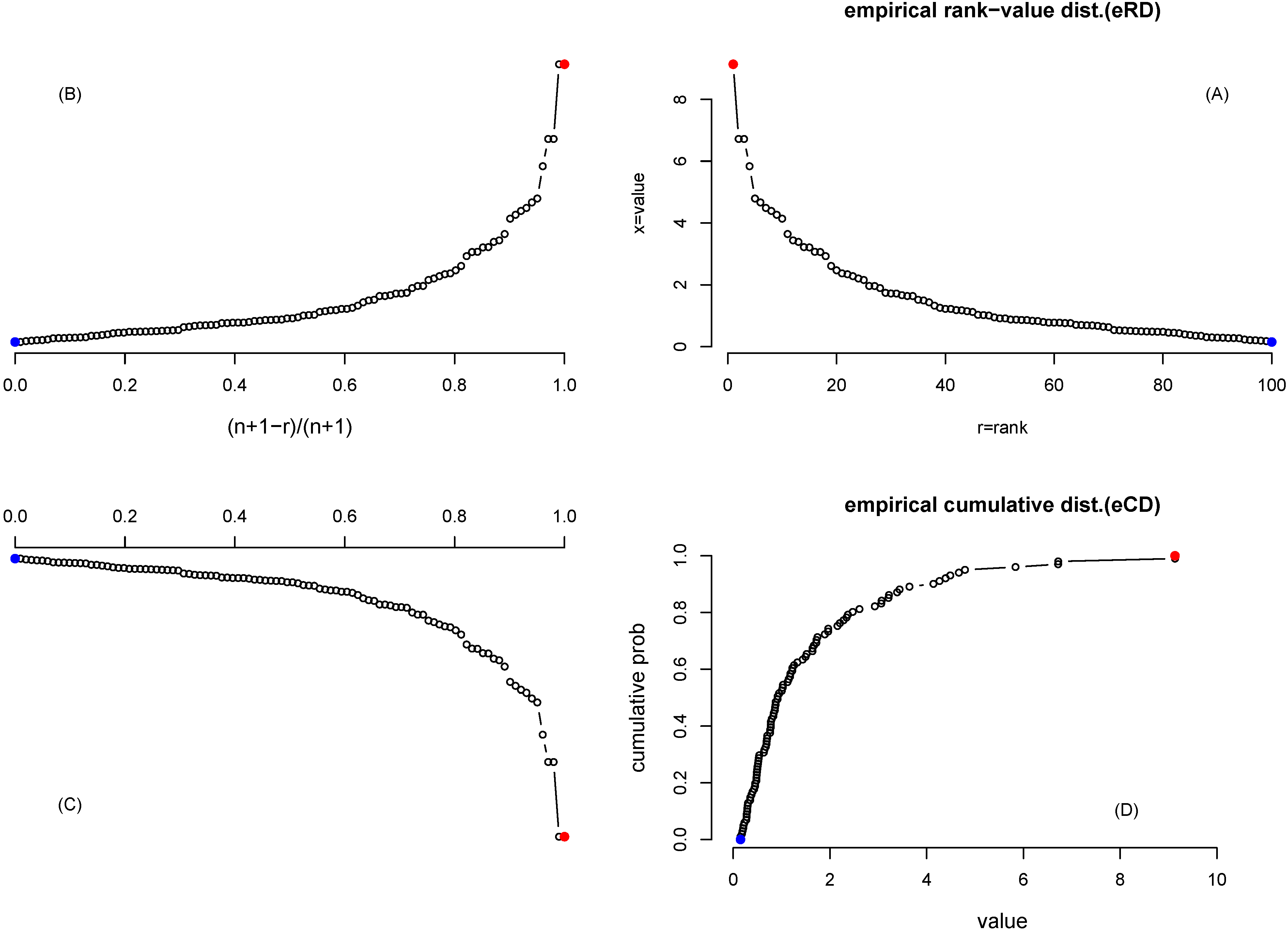
Figure 1 shows a step-to-step transformation (starting from the upper-right, counter-clockwise) from an eRD to an eCD, using
values randomly sampled from the log-normal distribution. One empirical rank-value distribution in
Figure 1(A) is transformed to
Figure 1(B) by a mirror image with respect to the
y-axis, plus a transformation of the
x-axis: the new
x-axis is reversed from the old
x-axis and is normalized to (0,1). The purpose of this operation is to start the empirical cumulation from the lowest ranking point.
Figure 1(C) is a mirror image of
Figure 1(B) with respect to
x-axis, and
Figure 1(D) is a counter-clockwise rotation of
Figure 1(C) of
.
Figure 1(D) is then the empirical cumulative distribution of this data set, which shows the proportion of values that are smaller than a threshold marked by the
x-axis. Actually, there is a simpler operation from
Figure 1(A) to
Figure 1(D): a clockwise rotation of
plus a reverse and a normalization of the old
x-axis to the new
y-axis in the range of (0,1).
The relationship between eRD and eCD has been discussed in the literature a number of times [
18,
19,
20,
21,
22,
23]. The reason we emphasize this relationship is to reinforce the understanding that a functional fitting of the rank-value distribution will correspond to a mathematical description of the empirical cumulative distribution, and vice versa. Since the derivative of the empirical cumulative distribution is the empirical probability density (ePD), we then have an estimation of ePD as well, even though it may not be in a close form. The relationship between an ePD and the true underlying distribution is always tricky [
6,
24].
The frequency spectrum (FS) [
6] is defined as the number of different events occurring with a given frequency. The cumulative sum of FS, called empirical structural type distribution (eSTD), is closely related to the empirical cumulative distribution. Generally speaking, eCD can be converted to eSTD by mirroring with respect to the
line, then rescale the new
y-axis from 1 to
n (see
Figure 1(D)). The situation is slightly more complicated when there are horizontal bars in eRD (equivalent to vertical lines in eCD) (see section 5). In that case, a horizontal bar is coverted to a point by its right end, before the mirror/rotation is carried out. We note that Alfred James Lotka used FS in his discovery of the power-law pattern in data [
22,
25].
Figure 1.
(A) log-normal distributed values being ranked (x-axis is the rank r, for the largest value, for the smallest value, y-axis is the value itself); (B) Mirror image of (A) with respect to the y-axis. Note that the new x-axis is both reversed and normalized (so that lowest ranking value at 0 and highest ranking value at 1); (C) Mirror image of (B) with respect of x-axis; (D) Rotation of (C) of . The highest ranking value is marked by the red color and the lowest ranking value by the blue color.-90
The Gusein-Zade and Weibull function introduced in section 1 can be understood by a reverse transformation from eCD to eRD. Suppose an eCD converges to 1 exponentially, which also describes the gap length distribution of a Poisson process with the mean gap length of
:
Similar to the survival curve in biostatistics [
26], eCD is a step function with
n vertical jumps. The lowest-ranking point (
) corresponds to the first step, with cumulative probability of
, and the highest-ranking point (
) corresponds to the last step with the cumulative probability of
. This can be used to rewrite Equation (
15) as:
or,
which is exactly Equation (
8). In data fitting, we treat any coefficient in the function as a parameter, thus
becomes
C. This rank-frequency distribution is exactly the same as the one proposed by Sabir Gusein-Zade [
13,
27,
28].
Suppose the CD approaches 1 in a stretched exponential relaxation [
29,
30]:
the converted RD is the Weibull function defined in Equation (
9) with
and
.
In general, any cumulative distribution of
f can be converted to RD by solving
f as a function of
r.
3. Ranked Letter Distribution
The frequency of letters in a language is of fundamental importance to communication and encryption. For example, the Morse code is designed so that the most common letters have the shortest codes. Shannon used the frequencies of letters as well as other units to study the redundancy and predictability of languages [
31]. It is well known that the letter “e" is the most frequent letter in English [
32,
33]. On the other hand, the most common letter in other languages can be different, e.g., “a" for Turkish, and “a", “e", “i" share the top ranks in Italian,
etc. (
http://en.wikipedia.org/wiki/Letter_frequency)
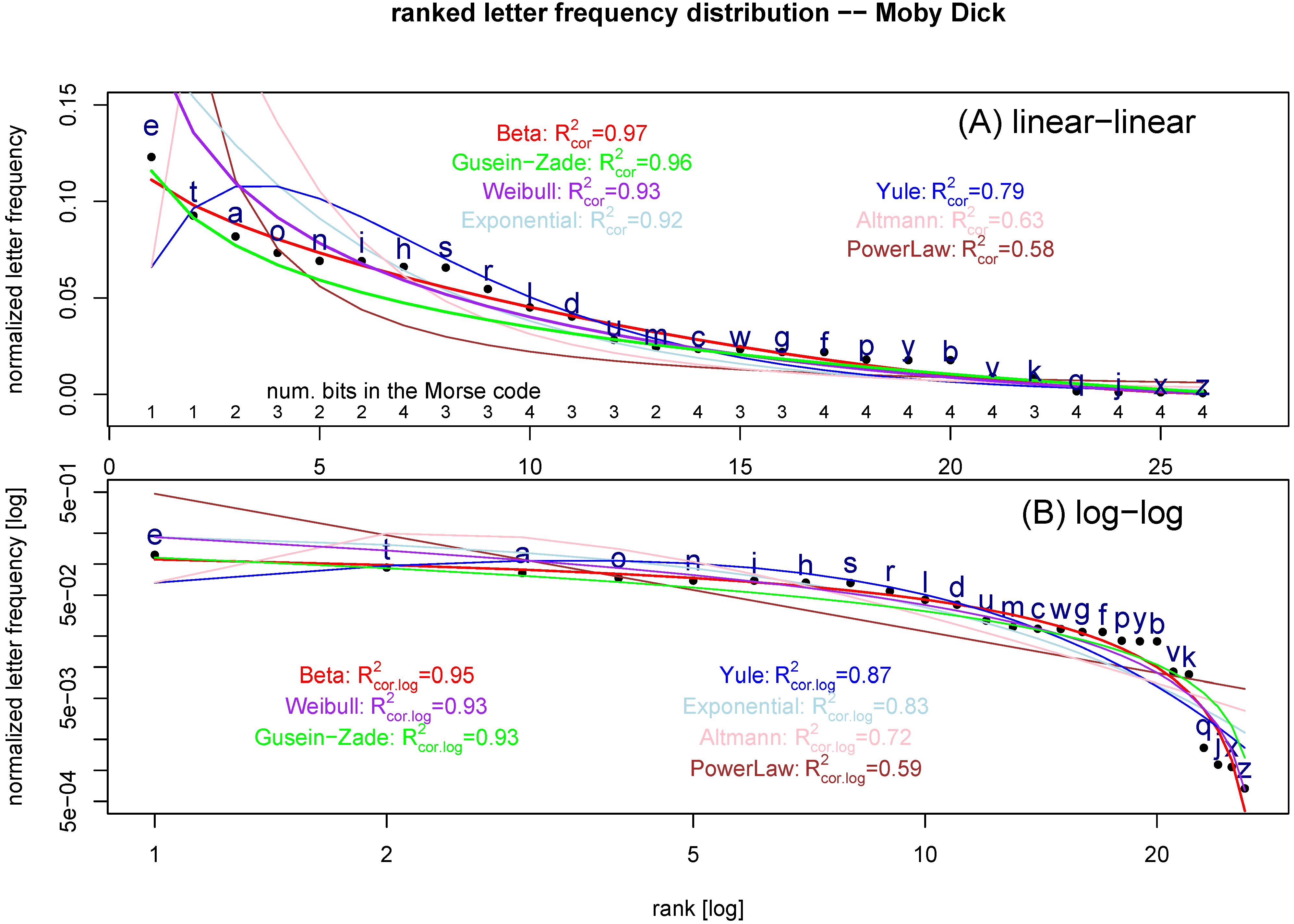
We plot the ranked letter frequencies in the text of
Moby Dick in
Figure 2 both in linear-linear and log-log scales (see
Appendix A for the source information). The number of bits in Morse code for these letters is also listed in
Figure 2(A), which does show the tendency of low number of bits for more commonly used letters. Seven fitting functions (one zero-parameter, three one-parameter, and three two-parameter functions) are applied (
Table 1). All can be framed in multiple regression (see
Appendix B for programming information).
The fitting of Gusein-Zade equation in a regression for the log-frequency data needs more explanation. From
Table 1, we see that there is no regression coefficient for the
term, and the only parameter to be estimated is the constant term. To show this fact, the regression model is re-written as:
From
Figure 2, it is clear that power-law, Altmann, and Yule functions do not fit the data as well as other functions. When the one-parameter functions are compared, exponential function clearly out-performs the power-law function.
For regression on the log-frequency data, SSE and AIC can be determined, and conclusion on which model is the best model can be reached.
Table 2 shows that Beta function is the best fitting function, followed by Weibull and Gusein-Zade function. The performance of Gusein-Zade function is impressive, considering that it has 2 fewer parameters than Beta and Weibull functions.
Another commonly used measure of fitting performance is
, which does ignore the issue of number of parameters.
can either be defined as the proportion of variance “explained” by the regression or defined as the squared correlation between the observed and the fitted values (see
Appendix C for more details).
Figure 2.
Ranked letter frequency distribution for the text of
Moby Dick (normalized so that the sum of all letter frequencies is equal to 1:
). (A) in the linear-linear scale, and (B) in log-log scale. Seven fitting functions (see
Table 1) are overlapped on the data: power-law function (brown,
), exponential (lightblue,
), Beta function (red,
), Yule function (blue,
), Gusein-Zade (green), Weibull (purple,
), and Altmann (pink,
). The number of bits in Morse code for the corresponding letter is written at the bottom of (A). The
values listed are
or
in Equation (
26).
The
values in
Table 2 show again that Beta function is the best fitting function, followed by Weibull and Gusein-Zade functions. The
and
for Gusein-Zade function is not equal because the variance decomposition does not hold true (
Appendix C) when Equation (
20) is converted back to the form of
.
When the regression is carried out in log-frequency scale, whereas the SSE and
is calculated in the scale, we do not expect the variance decomposition holds true, and do not expect
to be equal to
. The last two columns in
Table 2 shows SSE and
for these models when
y axis in linear scale. There are a few minor changes in the relative fitting performance among different functions. However, we caution in reading too much in these numbers as the parameter values are fitted to ensure the best performance in the log-frequency scale, not in the frequency scale.
Table 2.
Comparison of regression models in fitting ranked letter frequency distribution obtained from the text of Mody Dick. The regression is applied to the log-frequency scale (
Table 1).
: sum of squared error (Equation (
10)); ΔAIC: Akaike information criterion relative to the best model (whose AIC is set at 0) (Equation (
14));
: variance ratio Equation (
25);
: an alternative definition of
based on correlation (Equation (
26)). The SSE and
, based on the regression in the logarithmic scale, whereas applied to the linear
y scale, are shown in the last two columns.
Table 2.
Comparison of regression models in fitting ranked letter frequency distribution obtained from the text of Mody Dick. The regression is applied to the log-frequency scale (Table 1). : sum of squared error (Equation (10)); ΔAIC: Akaike information criterion relative to the best model (whose AIC is set at 0) (Equation (14)); : variance ratio Equation (25); : an alternative definition of based on correlation (Equation (26)). The SSE and , based on the regression in the logarithmic scale, whereas applied to the linear y scale, are shown in the last two columns.
| model | | log-scale | linear-scale |
|---|
| | | SSE | Δ AIC | | | SSE | |
| Gusein-Zade | 0 | 5.77 | 16.9 | 0.933 | 0.892 | .00196 | 0.962 |
| power-law | 1 | 22.2 | 53.9 | 0.586 | 0.586 | 0.145 | 0.580 |
| exponential | 1 | 8.91 | 30.2 | 0.834 | 0.834 | 0.0124 | 0.918 |
| Weibull | 1 | 3.59 | 6.52 | 0.933 | 0.933 | .00726 | 0.928 |
| Beta | 2 | 2.58 | 0 | 0.952 | 0.952 | .000716 | 0.973 |
| Yule | 2 | 6.66 | 24.6 | 0.876 | 0.876 | .00752 | 0.795 |
| Altmann | 2 | 14.83 | 47.4 | 0.723 | 0.723 | 0.0323 | 0.628 |
The fitted Beta function in
Figure 2(B) is:
i.e., the two parameters in Equation (1) are
and
. In [
34], the relative magnitude of
a and
b is used to measure the consistency to power-law behavior (
provides a confirming answer, and
does not). Equation (
21) indicates that the ranked letter frequency distribution in English is very different from a power-law function.
4. Ranked Inter-word Spacing Distribution
Motivated by level statistics in quantum disorder systems, it has been proposed that distance between successive occurrences of the same word might be related to whether or not that word plays an important role in the text (the so-called “keyword”) [
35,
36]. Similar studies of gap distributions are also common in bioinformatics, such as the in-frame start-to-stop codon distances (which defines “open reading frames”) [
37,
38] or in-frame stop-stop codon distances [
39]. In the example provided in [
36], for the text of Don Quijote, the function word “but” tends to be randomly scattered along the text, whereas the content word “Quijote” is more clustered. Here we will use the text of
Moby Dick to obtain the ranked nearest-neighbor distance distributions of selected words, and check which functions fit the data.
Figure 3 shows two ranked nearest-neighbor spacing distributions (after normalization) between a given word, one for a function word and another for a content word. The representative of function words is “THE” which is the most common word used in
Moby Dick. The representative of content words is “WHALE” which is the 23rd ranked word but the most common noun. The main conclusion in [
35,
36] is confirmed that function words such as THE tend to be evenly scattered whereas content words such as WHALE tends to be clustered, leaving huge gaps between clusters (and the low-rank-number spacings are much larger).
Figure 3.
Ranked nearest-neighbor spacing (normalized) between the word THE (in the unit of word) (A,B), and that between the word WHALE (C,D), in the text of Moby Dick. Both and -axis are in log scales. Six functions are used to fit the data: power-law (brown, (THE, weighted), (THE), (WHALE, weighted), (WHALE)), exponential (lightblue, (THE, weighted), (THE), (WHALE, weighted), (WHALE)), Beta (red, (THE, weighted), (THE), (WHALE, weighted), (WHALE) ), Yule (blue, (THE, weighted), (THE), (WHALE, weighted), (WHALE)), Weibull (purple, (THE, weighted), (THE), (WHALE, weighted), (WHALE) ), and Gusein-Zade functions (green), using either weighted least square regression (B,D) or regular least square regression (A,C). The weighting used is (r is the rank).-90
![]()
When a power-law function is applied to fit the inter-word spacings, the fitting performance is not good. In particular, it fails badly to fit the low-rank-number points (see the brown line in
Figure 3(A,C)). Since the density of points is denser at the tail of the ranking distribution, the least-square-fit regression result using all data points equally is not consistent with the visual impression in the log-log scale overlapping between the fitting line and the data.
There could be at least two solutions to this problem. The first solution is to use a subset of the data points so that these are evenly distributed in the log-transformed
x-axis. The second solution is to assign a weight to each point in the least-square fitting, such that the weight is smaller when the density of data points is higher in the log-transformed
x-axis. We adopt the second solution and choose a weight inversely proportional to the rank:
. This particular weight is chosen by some trials-and-errors process, and no theoretical justification will be provided in this paper. Weighting is allowed in the
R subroutine for linear regression (
Appendix B).
When the weighting option is chosen in power-law function, the regression line does indeed seem to pass through the low-rank-number points (brown line in
Figure 3(B,D)), although it still fails to fit the tail (high-rank number points) portion of the ranking distribution. Other functions, whose parameter values are determined by the weighted regression in log-spacing scale, are drawn in
Figure 3(B,D) as well: exponential, Beta, Yule, Weibull, and Gusein-Zade function
Table 3 summarizes the fitting results of these functions by SSE and AIC. Two sets of result are presented: one with the weight
and the other without. Interestingly, Yule function is the best fitting function in most situations, for both the function word “the" and content word “whale". The Beta function is the close second best function. The AIC difference between models for weighted regression is calculated by the formula in
Appendix E.
Table 3.
Comparison of regression models in fitting ranked inter-word spacing distributions obtained from the text of
Moby Dick for words THE and WHALE. The regression is applied to the log-distance scale (4th column of
Table 1). Two sets of result are presented: one for the weighted regression (weight
), another without weights. SSE: sum of squared error (Equation (
10)); ΔAIC: Akaike information criterion relative to the best model (whose AIC is set at 0) (Equation (
14)). One
(
in Equation (
31)) is listed in the last column.
Table 3.
Comparison of regression models in fitting ranked inter-word spacing distributions obtained from the text of Moby Dick for words THE and WHALE. The regression is applied to the log-distance scale (4th column of Table 1). Two sets of result are presented: one for the weighted regression (weight ), another without weights. SSE: sum of squared error (Equation (10)); ΔAIC: Akaike information criterion relative to the best model (whose AIC is set at 0) (Equation (14)). One ( in Equation (31)) is listed in the last column.
| word | model | | weighted regression | unweighted regression | |
|---|
| | | | SSE | Δ AIC | SSE | Δ AIC | |
| | Gusein | 0 | 0.701 | 25.9 | 5860.9 | 73588.2 | 0.933 |
| T | power-law | 1 | 0.947 | 31.0 | 1014.0 | 48720.0 | 0.909 |
| H | exponential | 1 | 2.49 | 40.8 | 295.1 | 31222.6 | 0.761 |
| E | Weibull | 1 | 0.698 | 27.9 | 1332.5 | 52591.9 | 0.933 |
| | Beta | 2 | 0.265 | 20.1 | 297.4 | 31334.1 | 0.975 |
| | Yule | 2 | 0.0366 | 0 | 32.6 | 0 | 0.996 |
| | Gusein | 0 | 3.83 | 18.7 | 155.2 | 2537.2 | 0.931 |
| W | power-law | 1 | 1.62 | 14.2 | 306.0 | 3320.2 | 0.919 |
| H | exponential | 1 | 3.58 | 20.2 | 122.4 | 2265.8 | 0.821 |
| A | Weibull | 1 | 1.38 | 12.9 | 155.2 | 2539.2 | 0.931 |
| L | Beta | 2 | 0.360 | 4.69 | 17.1 | 0 | 0.982 |
| E | Yule | 2 | 0.195 | 0 | 75.0 | 1703.2 | 0.990 |
Among several choices of
s (see
Appendix C,
Appendix D), we list
in
Table 3. The relative fitting performance judged by
is consistent with that by SSE and AIC. It is worth noting that the highest
values, which is achieved by the Yule function,
0.996 for word THE, 0.990 for word WHALE, are quite high. It indicates that Yule function fits the data very well.
It is proposed in [
35] that if a word is randomly distributed along the word sequence, it is a Poisson process and the nearest-neighbor spacing will follow an exponential distribution. That equation is exactly the Gusein-Zade function in Equation (
8). Both
Figure 3 and
Table 3 shows, however, that Gusein-Zade function is not the best fitting function when compared to others.
5. Revisiting Zipf’s Law
Ranked word frequency distribution in natural [
1] and artificial languages [
40] follows a reasonably good power-law, especially when only the low-rank-number words are fitted. Ranking words by their frequency of usage has practical applications, for example, it may establish the priorities in learning a language [
41]. However, the fitting by a power-law function for the whole range of ranks is by no mean perfect. In [
42], it was suggested that two power-law fitting with two different scaling exponents are needed to fit the ranked word frequencies. In a more striking illustration [
43], 42 million words (tokens) from Wall Street Journal were used to draw the ranked word frequencies, and it deviate from the Zipf’s law at
.
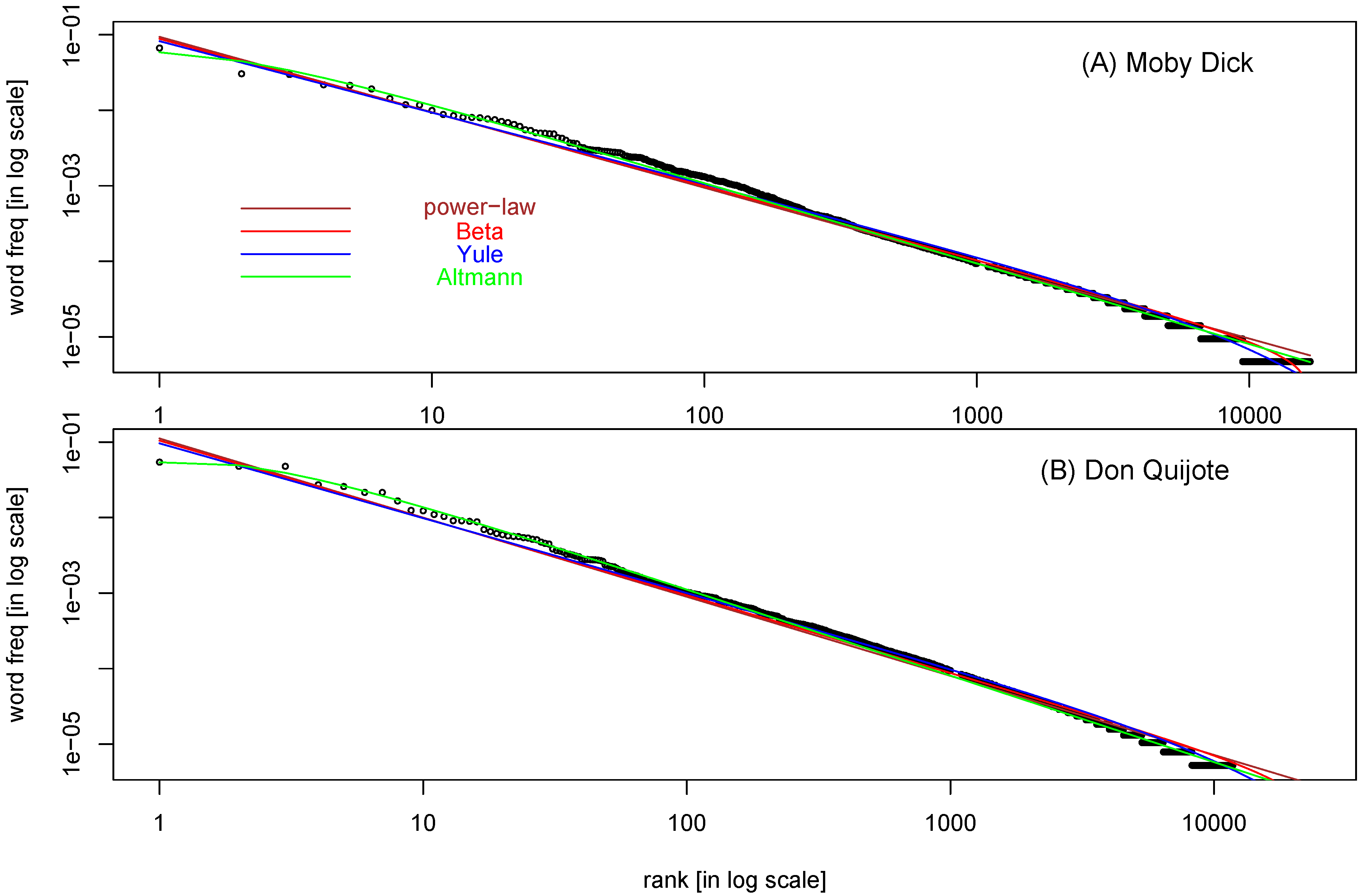
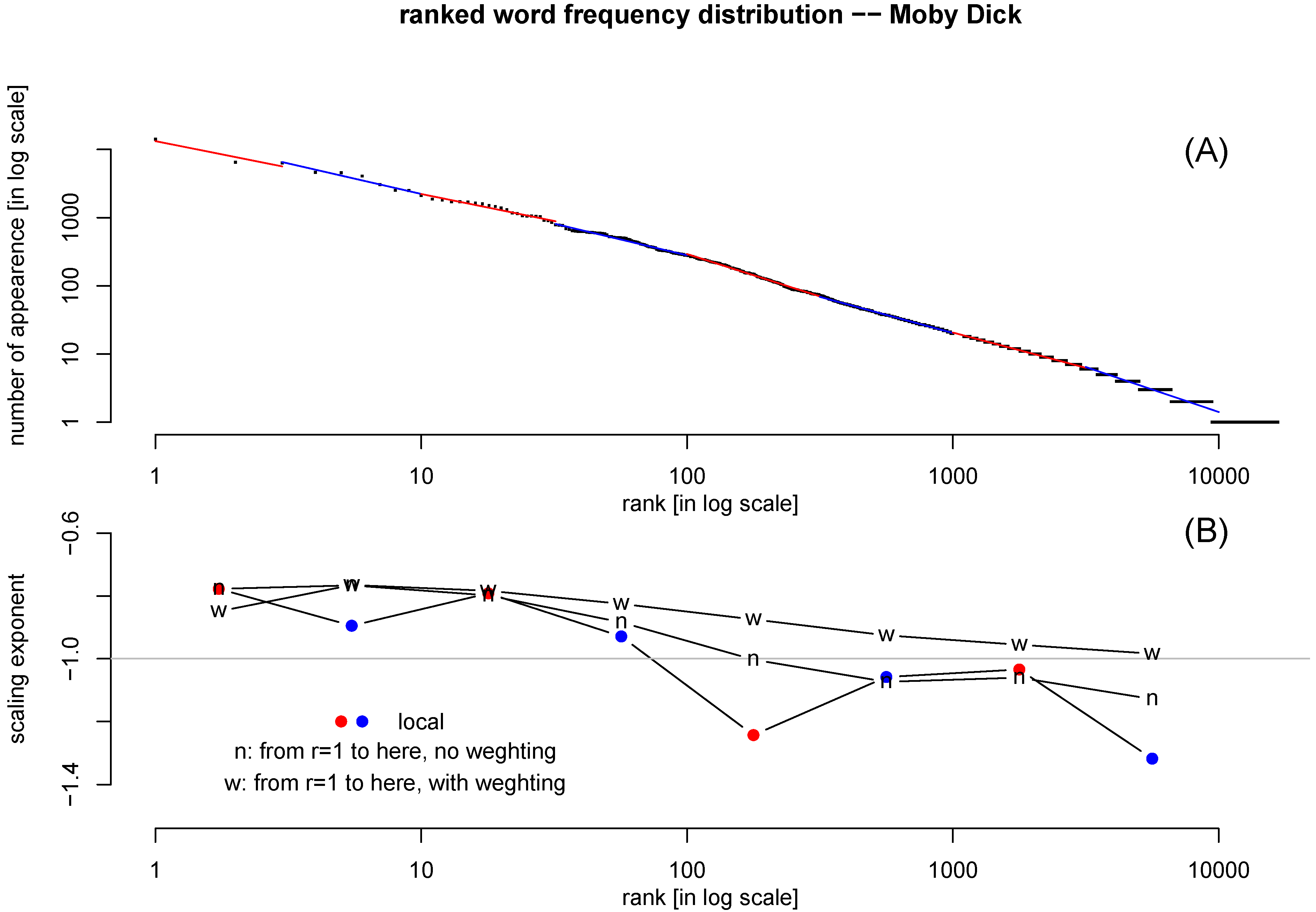
Figure 4(A) shows the ranked word frequency distribution for the text
Moby Dick. In order to examine more closely how good Zipf’s law fits the data, we carry about three regression analyses: one is a local regression using only points whose rank is within certain range; the second is a regression for all points whose ranking number is lower (
) than certain value. That regression is repeated with the weight of
.
Figure 4.
(A) Ranked word frequency distribution of text Moby Dick, in log-log scale. The number of word type is 16713, and the number token is 212791. Points within certain rank range are fitted with power-law locally, alternately colored by red and blue. (B) The slope of the local regression line (red/blue): the slope of regression for all points higher than certain rank (): without weight (“n") and with weight () (“w").-90
The scaling exponents from these three types of regressions are plotted in
Figure 4(B). It is clear that the slope is becoming steeper towards the tail (high-rank-number words). The regression with weight manages to slow down the increase of the slope, as the points near the tail are weighted down. Still, the slope is not a constant. The slope of
as expected by the Zipf’s law is marked in
Figure 4(B) as a reference.
Figure 4 confirms the previous observations that Zipf’s law is not a perfect fit of the ranked word frequency distribution in the full rank range [
42,
43].
This leaves room for improvement by a two-parameter fitting function.
Figure 5 shows the results of three 2-parameter fitting functions (all with weight
) plus that of power-law function, one for words frequency in
Moby Dick and another for Don Quijote (see
Appendix A for source information). Exponential function, Gusein and Weibull function all fit the data badly, so these are not included in the plot.
Table 4 shows SSE and ΔAIC (relative to the best model) of these four functions, in both weighted and unweighted regression. For weighted regression, Altmann function is the best model, although other three functions are not far behind. For unweighted regression, Beta function is the best model. The reason for this difference might be due to the ability of Altmann function to make nonlinear (in log-log plot) turn at the head area of the curve (low-rank-number), and that of the Beta function at the tail area (high-rank-number).
Table 4 also shows that ranking of functions by
values is consistent with that by SSE.
We may conclude from
Table 4 that it is worthwhile to use two-parameter models, as all three (Beta, Yule, and Altmann function) outperform the Zipf’s law, even if not by much. One important point made in [
6] is that when dealing with the word frequency distribution, due to the presence of “large number of rare words” [
6,
24], the length of the text may affect the result. Consequently, it is preferable to check the obtained word statistics as a function of the sample size.
In order to check whether the conclusion that two-parameter models outperform Zipf’s law is still true at a different sample size, we split the Don Quijote into two books: El ingenioso hidalgo don Quijote de la Mancha, and Segunda parte del ingenioso caballero don Quijote de la Mancha. The SSE and relative AIC result of these two books are shown in
Table 4. The main conclusion that Altmann function is the best model in weighted regression, and Beta function is the best in unweighted regression, remain the same.
Figure 5.
Ranked word frequency (normalized) in the English text of
Moby Dick (MD) (A), and the Spanish text of Don Quijote (DQ) (B). The following weighted regressions are applied and the resulting fitting lines are shown (
Table 1): power-law function or Zipf’s law (brown,
(MD, weighted),
(DQ, weighted) ), Beta function (red,
(MD, weighted),
(DQ, weighted) ), Yule function (blue,
(MD, weighted),
(DQ, weighted) ), and Menzerath-Altmann function (green,
(MD, weighted),
(DQ, weighted)).-90
6. Discussion
It is natural to add more parameters to models when they fail to fit satisfactorily certain sets of data (e.g., [
44]). Nevertheless, if the mathematicians’ task were only to fit the data, then with as many parameters as the points in the dataset it would be possible in principle to fit anything but the resulting model would be useless because it would be good only for a particular set of data. The goal should then be to find a balance between the extremes of too few parameters and bad fittings and too many parameters and overfitting.
For many linguistic data, one-parameter functions perform reasonably well, but when analyzing large datasets there are some discrepancies at the extremes of the abscissae. It is easy to understand why we would like to try some more parameters starting with two parameter models. These models have not been extensively used partly because of a lack of critical comparison among them, and partly because their performance may depend on particular dataset used.
Table 4.
Comparison of regression models in fitting ranked word frequency distributions obtained from the English text of
Moby Dick, and the Spanish text of Don Quijote. The two books of Don Quijote are also separated for additional analysis with the goal of checking sample-size effect. The regression is applied to the log-distance scale (4th column of
Table 1). Two sets of result are presented: one for the weighted regression (weight
), another without weights. SSE: sum of squared error (Equation (
10)); ΔAIC: Akaike information criterion relative to the best model (whose AIC is set at 0) (Equation (
14)). The last column is
in Equation (
31).
Table 4.
Comparison of regression models in fitting ranked word frequency distributions obtained from the English text of Moby Dick, and the Spanish text of Don Quijote. The two books of Don Quijote are also separated for additional analysis with the goal of checking sample-size effect. The regression is applied to the log-distance scale (4th column of Table 1). Two sets of result are presented: one for the weighted regression (weight ), another without weights. SSE: sum of squared error (Equation (10)); ΔAIC: Akaike information criterion relative to the best model (whose AIC is set at 0) (Equation (14)). The last column is in Equation (31).
| data | model | | weighted regression | unweighted regression | |
|---|
| | | | SSE | ΔAIC | SSE | ΔAIC | |
| | power-law | 1 | 0.656 | 7.54 | 452.7 | 551.7 | 0.993 |
| Moby | Beta | 2 | 0.523 | 7.21 | 438.0 | 0 | 0.994 |
| Dick | Yule | 2 | 0.369 | 3.69 | 442.8 | 184.0 | 0.996 |
| | Altmann | 2 | 0.260 | 0 | 441.2 | 120.3 | 0.997 |
| | power-law | 1 | 1.10 | 17.9 | 783.8 | 6018.2 | 0.990 |
| Don | Beta | 2 | 0.950 | 18.3 | 603.4 | 0 | 0.991 |
| Quijote | Yule | 2 | 0.721 | 15.3 | 748.7 | 4959.5 | 0.993 |
| | Altmann | 2 | 0.170 | 0 | 771.5 | 5654.3 | 0.998 |
| | power-law | 1 | 0.831 | 16.3 | 560.9 | 6045.8 | 0.991 |
| Don | Beta | 2 | 0.751 | 17.3 | 377.2 | 0 | 0.992 |
| Quijote | Yule | 2 | 0.592 | 14.8 | 483.0 | 3767.8 | 0.994 |
| book-1 | Altmann | 2 | 0.138 | 0 | 556.9 | 5937.7 | 0.999 |
| | power-law | 1 | 0.964 | 19.0 | 591.2 | 6861.8 | 0.990 |
| Don | Beta | 2 | 0.899 | 20.3 | 391.0 | 0 | 0.991 |
| Quijote | Yule | 2 | 0.758 | 18.5 | 499.1 | 4053.0 | 0.992 |
| book-2 | Altmann | 2 | 0.125 | 0 | 588.7 | 6791.9 | 0.999 |
For ranked letter frequency data, because the range of abscissae is short, the difference between various fitting functions can be small. Only when the independent variable range is expanded, could we see a divergence among different functions.
In this paper, we only limit ourselves to regression models on the log-frequency-log-rank scale. And it is interesting to find Beta function outperform the Gusein-Zade function traditionally applied in the letter frequency distribution [
27]. Further analyses are needed, both by using other datasets and by using regression in the frequency scale, to have more confidence of the conclusion reached here.
For inter-word spacing distribution, if a word appears in the text randomly, its probability distribution is a geometric distribution [
35]. Geometric distribution is the discrete version of exponential distribution, and because integral of an exponential function is still exponential, by the method in section 2, we expect the Gusein-Zade function to fit the ranked data well. It is again interesting that the best fitting function is not Gusein-Zade function, but Yule function.
The word frequency distribution is one of the most studied linguistic data, following the works by Zipf [
1], and with tremendous amount of knowledge being accumulated on this topic [
6]. Mandelbrot function is an example of extending one-parameter to two-parameter in fitting word frequency distribution [
11]. Most usage of two-parameter models in linguistic data is perhaps on the phoneme distribution [
10,
29]. In our analysis, although several two-parameter models outperform the power-law function, the Zipf’s law is still reasonably good.
In this paper we reveal some technical subtleties in fitting a function modified from a power-law function. Since power-law function is a linear function when both axes are in logarithmic scales, it is much easier to apply a linear regression on the log-transformed data. However, in the log-log plot, the density of data points at the low-ranking end (large r values) is much higher, even though their contribution to a visual impression is much less than their proportions. Whether or not we put a lesser weight on these points may affect the data fitting result.
Another issue not yet addressed in this paper is that a logarithmic transformation changes the data to another dataset, and the fitting result can be different from that before the logarithmic transformation. Since one major purpose of the logarithmic transformation is to apply an easier linear regression, in order to avoid a data transformation, non-linear regression is needed. Such analysis will be delayed to a future study.
Fitting linguistic data with more than two parameters (e.g., 3, 4) remains a possibility for future studies. However, for the three types of data considered here, the best
’s are all larger than 0.95 using two-parameter functions, and there is no obvious systematic deviations. Two-parameter functions seem to achieve a good balance between under- and over-fittings. As in any statistical modeling, more does not always means better [
45].
In conclusion, even though we have not exhausted all two-parameter functions in fitting ranked linguistic data, we at least put some of them together at one place that were used to be scattered in the literature. Some preliminary conclusions have been reached: among the functions we studied, and by fitting the log-transformed data, Beta function is the best fitting function for English letter frequency distribution, Yule is the best fitting function for inter-word spacing distribution, and Altmann function fits the word frequency distribution slightly better than others. However, these specific conclusions need confirmation in more datasets. It is important to emphasize the fact that a good statistical fitting could lead to a good phenomenological or first-principles approach to the same problem. We hope that this paper could contribute to pave the way in this direction for linguistic data.

