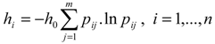
Imprecise Shannon’s Entropy and Multi Attribute Decision Making

Farhad Hosseinzadeh Lotfi; Reza Fallahnejad

doi:10.3390/e12010053

and

Department of Mathematics, Science & Research Branch, Islamic Azad University (IAU), Tehran, Iran

^*

Author to whom correspondence should be addressed.

Entropy2010, 12(1), 53-62;https://doi.org/10.3390/e12010053

Version Notes

Order Reprints

Abstract

Finding the appropriate weight for each criterion is one of the main points in Multi Attribute Decision Making (MADM) problems. Shannon’s entropy method is one of the various methods for finding weights discussed in the literature. However, in many real life problems, the data for the decision making processes cannot be measured precisely and there may be some other types of data, for instance, interval data and fuzzy data. The goal of this paper is the extension of the Shannon entropy method for the imprecise data, especially interval and fuzzy data cases.

Keywords:

multi attribute decision making; entropy; imprecise data

MSC Codes:

90B50; 90C29; 90C70

1. Introduction

Multiple attribute decision making (MADM) refers to making preference decisions (e.g., evaluation, prioritization, and selection) over the available alternatives that are characterized by multiple, usually conflicting, attributes. The structure of the alternative performance matrix is depicted in Table 1, where x_ij is the rating of alternative i with respect to criterion j and w_j is the weight of criterion j (in this paper, we consider the case that the rating of alternative i with respect to criterion j is non-negative).

Table 1. Structure of the alternative performance matrix.

**Table 1.** Structure of the alternative performance matrix.
	Criterion 1	Criterion 2	…	Criterion n
Alternative 1	X₁₁	X₁₂	…	X_1n
Alternative 2	X₂₁	X₂₂	…	X_2n
⋮	⋮	⋮	⋮	⋮
Alternative m	X_m1	X_m2	…	X_mn
	W₁	W₂	…	W_n

Since each criterion has a different meaning, it cannot be assumed that they all have equal weights, and as a result, finding the appropriate weight for each criterion is one the main points in MADM. Various methods for finding weights can be found in the literature and most of them can be categorized into two groups: subjective and objective weights. Subjective weights are determined only according to the preference decision makers. The AHP method [1], weighted least squares method [2] and Delphi method [3] belong in this category. The objective methods determine weights by solving mathematical models without any consideration of the decision maker’s preferences, for example, the entropy method, multiple objective programming [4,5], principal element analysis [5], etc. Since in the most real problems, the decision maker’s expertise and judgment should be taken into account, subjective weighting may be preferable, but when obtaining such reliable subjective weights is difficult, the use of objective weights is useful. One of the objective weighting measures which has been proposed by researchers is the Shannon entropy concept [6]. Entropy concept was used in various scientific fields. The concept of Shannon’s entropy has an important role in information theory and is used to refer to a general measure of uncertainty. In transportation models, entropy is acted as a measure of dispersal of trips between origin and destinations [7]. In physics, the word entropy has important physical implications as the amount of “disorder” of a system [7]. Also the entropy associated with an event is a measure of the degree of randomness in the event. Entropy has also been concerned as a measure of fuzziness [8]. In MADM the greater the value of the entropy corresponding to an special attribute, which imply the smaller attribute’s weight, the less the discriminate power of that attribute in decision making process.

In many real life problems, the data of the decision making processes cannot be measured precisely and there may be some other types of data, for instance interval data and fuzzy data. In other words, the decision maker would prefer to say his/her point of view in these forms rather than a real number because of the uncertainty and the lack of certain data, especially when data are known to lie within bounded variables, or when facing missing data, judgment data, etc. In MADM it is most probable that we confront such a case, so finding a suitable weight is an important problem. It is logical that when data are imprecise, weights be imprecise too. In this paper we present a method for solving MADM problems by entropy method consisting of interval data. In this method the weight, which is obtained for each alternative, will be an interval number. We apply the Sengupta approach mentioned in [9] to compare the interval scores we have found.

This paper has been organized as follows: In Section 2 the MADM problem is presented with interval data. Then Entropy method is extended for the interval data. In the same section we will also show that if all of the alternatives have deterministic data, then the interval entropy weight leads to the usual entropy weight. In Section 3, by using α-level set, we will obtain interval weight for fuzzy MADM problem in different levels of confidence. We will also use the data of an empirical example for more explanation and showing the validation of the proposed method. The final section will be the conclusion.

2. Interval Shannon’s Entropy

2.1. Method

As noted before, Shannon’s entropy is a well known method in obtaining the weights for an MADM problem especially when obtaining a suitable weight based on the preferences and DM experiments are not possible. The original procedure of Shannon’s entropy can be expressed in a series of steps:

S1: Normalize the decision matrix.

Set

The raw data are normalized to eliminate anomalies with different measurement units and scales. This process transforms different scales and units among various criteria into common measurable units to allow for comparisons of different criteria.

S2: Compute entropy h_i as Entropy 12 00053 i002

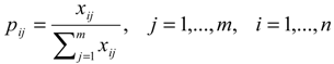
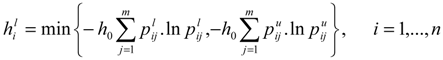
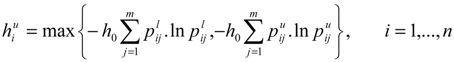
, where h₀ is the entropy constant and is equal to (ln m)^-1, and p_ij .ln p_ij is defined as 0 if p_ij = 0.

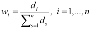S3: Set d_i = 1 − h_i , i = 1,...,n as the degree of diversification.

S4: Set Entropy 12 00053 i003

as the degree of importance of attribute i.

Now suppose that determining the exact value of the elements of decision matrix is difficult and, as a result, their values are considered as intervals. The structure of the alternative performance matrix in interval data case is expressed as shown in Table 2, where [

x_{i j}^{l}, x_{i j}^{u}

] is the rating of alternative i with respect to criterion j, [

w_{j}^{l}, w_{j}^{u}

] is the weight of criterion j:

Table 2. Structure of the alternative performance when data are intervalled.

**Table 2.** Structure of the alternative performance when data are intervalled.
	Criterion 1	Criterion 2	…	Criterion n
Alternative 1	[ $x_{11}^{l}, x_{11}^{u}$ ]	[ $x_{12}^{l}, x_{12}^{u}$ ]	...	[ $x_{1 n}^{l}, x_{1 n}^{u}$ ]
Alternative 2	[ $x_{21}^{l}, x_{21}^{u}$ ]	[ $x_{22}^{l}, x_{22}^{u}$ ]	...	[ $x_{2 n}^{l}, x_{2 n}^{u}$ ]
⋮	⋮	⋮		⋮
Alternative m	[ $x_{m 1}^{l}, x_{m 1}^{u}$ ]	[ $x_{m 2}^{l}, x_{m 2}^{u}$ ]	...	[ $x_{m n}^{l}, x_{m n}^{u}$ ]
	[ $w_{1}^{l}, w_{1}^{u}$ ]	[ $w_{2}^{l}, w_{2}^{u}$ ]	...	[ $w_{n}^{l}, w_{n}^{u}$ ]

When there is interval data, and considering the fact that the value of each alternative with respect to each criterion can change within a range and have different behaviors, it is logically better that weights change in different situations as well (note that here the DM knows that the exact/real value of a criterion is within its data interval and the probability of each point to be the exact value is the same—in other words, a uniform distribution of the interval data is assumed). Therefore, we try to extend Shannon’s entropy for these interval data.

Proposed Approach

S’1: The normalized values

p_{i j}^{l}

and

p_{i j}^{u}

are calculated as:

S’2: Lower bound

h_{i}^{l}

and upper bound

h_{i}^{u}

of interval entropy can be obtained by:

where h₀ is equal to (ln m)^-1, and

p_{i j}^{l} . \ln p_{i j}^{l}

or

p_{i j}^{u} . \ln p_{i j}^{u}

is defined as 0 if

p_{i j}^{l} = 0

or

p_{i j}^{u} = 0

.

S’3: Set the lower and the upper bound of the interval of diversification

d_{i}^{l}

and

d_{i}^{u}

as the degree of diversification as follows:

S’4: Set Entropy 12 00053 i008

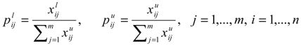
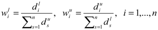as the lower and upper bound of interval weight of attribute i.

Theorem.

The inequality Entropy 12 00053 i009

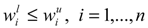is held.

Proof.

By using the definition of

h_{i}^{l}

and

h_{i}^{u}

in the second step of the proposed approach, it is clear that

h_{i}^{l} \leq h_{i}^{u}

. Also referring to the definition of

d_{i}^{l}

and

d_{i}^{u}

we have

. So

and

. Therefore Entropy 12 00053 i009

.

Definition. We name the interval Entropy 12 00053 i013

as the weight of i’th criterion obtained from interval entropy method. Notice that if all of the alternatives have deterministic data, then we have

x_{i j}^{l} = x_{i j}^{u}

and also

p_{i j}^{l} = p_{i j}^{u}

. So we have

h_{i}^{l} = h_{i}^{u}

and therefore

d_{i}^{l} = d_{i}^{u}

, then

w_{i}^{l} = w_{i}^{u}

(the basic entropy weight). It means if all of the alternatives have deterministic data, then the interval entropy weight leads to the usual entropy weight. As a result, the entropy weight in the case of interval data as the proposed method is well defined, but if at least one of the numbers is interval, all weights will be in the interval form, even for the criteria with crisp data. The reason is that the final entropy weight is dependent on the degree of diversification (d_i) of all criteria based upon the forth step of the entropy method ( Entropy 12 00053 i014

). So, if a criterion is in the interval form, its degree of diversification will be obtained in the interval form too. Therefore, the weight of crisp criteria will alter based on the alteration of the degree of diversification of an interval criterion in its interval degree of diversification.

2.2. Comparing interval weights

After determining the weights in interval form by using the proposed method, we must rank them. In other words, when considering two interval numbers; we want to know which one is “greater” or “smaller”. Various methods can be found in the literature for ranking interval data, each of which is based on a certain theory (for example see [9,10,11,12,13,14]). In this paper we use Sengupta’s approach [9]. As we know, interval data can be shown by their first and last points. But an interval number can be shown by its mid-point and its half-width. Sengupta’s approach compares two intervals based upon those. Sengupta and Pal introduced the acceptability function to compare two interval numbers D and E as follows: Entropy 12 00053 i015

where m (D), m (E) are the mid-points of interval numbers D and E, and w (D), w (E) are the half-width of D and E. A_(≺) may be interpreted as the ‘‘first interval to be inferior to the second interval’’. This procedure states that between two interval numbers with the same mid-point, the less uncertain interval will be the best choice for both of maximization and minimization purposes.

2.3. A numerical example

In this section, the steps of the proposed method are described with a simple example. Suppose that there is an MADM problem with six alternatives and four criteria. Data are presented in Table 3.

Table 3. The data of alternatives.

**Table 3.** The data of alternatives.
	C1	C2	C3	C4
A1	1451	[2551,3118]	[40,50]	[153,187]
A2	843	[3742,4573]	[63,77]	[459,561]
A3	1125	[3312,4049]	[48,58]	[153,187]
A4	55	[5309,6488]	[72,88]	[347,426]
A5	356	[3709,4534]	[59,71]	[151,189]
A6	391	[4884,5969]	[72,88]	[388,474]

As we can see, the first criterion is in the crisp form whereas other criteria are intervals. We want to obtain a weight for each criterion by using the proposed approach. In Table 4 the normalized data are presented.

Table 4. The normalized rates.

**Table 4.** The normalized rates.
C1	C2	C3	C4
0.343905	[0.088491,0.108578]	[0.092623,0.115778]	[0.06442,0.343905]
0.199703	[0.130293,0.159066]	[0.145396,0.178244]	[0.193756,0.199703]
0.266601	[0.115092,0.140608]	[0.110932,0.134626]	[0.06442,0.266601]
0.012884	[0.184582,0.225841]	[0.166397,0.203554]	[0.146184,0.012884]
0.084242	[0.129207,0.15798]	[0.136241,0.164243]	[0.063429,0.084242]
0.092666	[0.169924,0.207926]	[0.166397,0.203554]	[0.163528,0.092666]

In the first row of Table 5, interval entropy of each criterion obtained in the second step (S’2) can be seen. The closer the entropy of a criterion to 1, the less important the criterion. In the second and the third rows of Table 5, the degree of diversification and the weight of each criterion are mentioned. As can be seen, the corresponding weight to the first criterion, which is in the crisp form, is interval. As mentioned before, since other criteria have interval diversification, as their diversification change between intervals, the weight of the first criterion will change within an interval too. Finally we applied Sengupta approaches to rank the criteria. Mid-points and half-widths of interval weights that are used to obtain the final rank of each criterion by using the acceptability function can be seen in raw 4 and raw 5 of Table 5. To determine the rank of criterion C1 for example, we use acceptability functions for intervals corresponding to C1 and C2, C1 and C3 and also C1 and C4. The obtained values are –0.9461898, –0.9729971 and 0.35378407, respectively. We see that the rank of C1 is just better than the rank of C4. Therefore, C1 locates at rank 3. Other criteria can be ranked in the same way. For problems with more complexity, with a small program (for example Excel) we can determine the rank of each criterion. In the last row of Table 5, the rank of each criterion can be seen.

Table 5. Entropy, degree of diversification, weight and rank.

**Table 5.** Entropy, degree of diversification, weight and rank.
	C1	C2	C3	C4
Entropy	0.851761	[0.896549,0.984209]	[0.900264,0.988816]	[0.794438,0.851761]
Degree of Diversification	0.148239	[0.015791,0.103451]	[0.011184,0.099736]	[0.148239,0.205562]
Weight	[0.266143,0.458301]	[0.028352,0.319835]	[0.020079,0.308348]	[0.266143,0.635525]
Mid-point	0.362222	0.174093	0.164213	0.450834
Half-width	0.096079	0.145742	0.144135	0.184691
Rank	2	3	4	1

3. Fuzzy Shannon’s Entropy

3.1. Fuzzy Shannon’s entropy based on α-level sets

In real decision making problem, a lot for data happens to be of fuzzy type. The structure of the alternative performance matrix in fuzzy data case is expressed as shown in Table 6, where

{\tilde{x}}_{i j}

is the rating of alternative i with respect to criterion j, and

{\tilde{w}}_{j}

is the weight of criterion j:

Table 6. Structure of the alternative performance in the case of fuzzy data.

**Table 6.** Structure of the alternative performance in the case of fuzzy data.
	Criterion 1	Criterion 2	…	Criterion n
Alternative 1	${\tilde{x}}_{11}$	${\tilde{x}}_{12}$	...	${\tilde{x}}_{1 n}$
Alternative 2	${\tilde{x}}_{21}$	${\tilde{x}}_{22}$	...	${\tilde{x}}_{2 n}$
⋮	⋮	⋮	⋮	⋮
Alternative m	${\tilde{x}}_{m 1}$	${\tilde{x}}_{m 2}$	...	${\tilde{x}}_{m n}$
	${\tilde{w}}_{1}$	${\tilde{w}}_{2}$	...	${\tilde{w}}_{n}$

In the case where all fuzzy data are expressed in triangular and trapezoidal fuzzy numbers, several approaches have been proposed to deal with the fuzzy data. Fuzzy data will be transformed into interval data in this paper by using the α-level sets.

Definition (α-level sets). The α-level set of a fuzzy variable

{\tilde{x}}_{i j}

is defined by a set of elements that belong to the fuzzy variable

{\tilde{x}}_{i j}

with membership of at least α i.e., Entropy 12 00053 i016

.

The α-level set can also be expressed in the following interval form:

where 0 < α ≤ 1. By setting different levels of confidence, namely 1 − α, fuzzy data are accordingly transformed into different α-level sets Entropy 12 00053 i018

, which are all intervals. Now by using the proposed method in the previous section, we can obtain an interval weight for each α-level set. We name the entropy weight for the i’th fuzzy criterion in α-level as Entropy 12 00053 i019

. Now by using every interval ranking method, we can rank all fuzzy criteria in every α-level set. In what follows, we find the weights for the criteria of a real MADM problem.

3.2. Empirical example

Consider Table 7 in which there are seven alternatives and 16 criteria. Data are taken from [15]. Data are fuzzy triangular numbers in the form of (a,b,c), where the first, second and third components display the left, center and right side of the related numbers. We used the proposed method for five level sets, 0.1, 0.3, 0.5, 0.7 and 0.9. The obtained weights and the corresponding rank of each criterion for different α-level sets are presented in Table 8. As can be seen in Table 8, the rankings under different α-levels might be quite different. In this situation, the overall ranking cannot be easily observed. In order to generate an overall ranking, choosing a trade-off between the precision and the confidence is suggested. A higher α means precision of the interval chosen and a lower α means a higher confidence in the result. A risk-averse assessor or DM might choose a high alpha because of strong dislike of uncertainty (fuzziness), while a risk-taking assessor or DM might prefer a low alpha because of seeking risk. In addition, weighted averaging of the interval weights by using alpha as weight is suggested. After obtaining the weighted average, ranks can be obtained by different approaches, for example Sengupta approach.

Table 7. The data of alternatives (Empirical Example).

**Table 7.** The data of alternatives (Empirical Example).
	A1	A2	A3	A4	A5	A6	A7
C1	(3.400, 5.400, 7.400)	(3.799, 5.800, 7.800)	(4.333, 6.333, 8.266)	(6.199, 8.199, 9.600)	(2.599, 4.599, 6.599)	(5.266, 7.266, 9.066)	(6.733, 8.733, 9.866)
C2	(1.799, 3.799, 5.800)	(3.799, 5.800, 7.800)	(5.533, 7.533, 9.266)	(7, 9,10)	(3, 5,7)	(5.533, 7.533, 9.266)	(3.799, 5.800, 7.800)
C3	(3.799, 5.800, 7.733)	(3.799, 5.800, 7.733)	(3.799, 5.800, 7.733)	(6.333, 8.333, 9.600)	(3.799, 5.800, 7.733)	(5.266, 7.266, 9)	(5.133, 7.133, 8.866)
C4	(4.066, 6.066, 8.066)	(5.800, 7.800, 9.333)	(5.800, 7.800, 9.333)	(5.800, 7.800, 9.333)	(1.933, 3.933, 5.933)	(5.800, 7.800, 9.333)	(4.066, 6.066, 8.066)
C5	(4.599, 6.599, 8.533)	(5.266, 7.266, 8.933)	(5.266, 7.266, 8.933)	(5.266, 7.266, 8.933)	(3.133, 5.133, 7)	(5.266, 7.266, 8.933)	(4.599, 6.599, 8.533)
C6	(2.866, 4.866, 6.866)	(4.866, 6.866, 8.666)	(5.400, 7.400, 9.066)	(5.533, 7.533, 9.199)	(3.400, 5.400, 7.400)	(6.733, 8.733, 9.866)	(3.799, 5.800, 7.733)
C7	(2.466, 4.466, 6.466)	(4.866, 6.866, 8.666)	(4.866, 6.866, 8.666)	(5.533, 7.533, 9.133)	(4.466, 6.466, 8.399)	(6.466, 8.466, 9.600)	(3.400, 5.400, 7.333)
C8	(4.466, 6.466, 8.199)	(4.466, 6.466, 8.199)	(4.466, 6.466, 8.199)	(4.466, 6.466, 8.199)	(2.599, 4.599, 6.599)	(2.599, 4.599, 6.599)	(4.466, 6.466, 8.199)
C9	(2.333, 4.333, 6.333)	(5.133, 7.133, 8.866)	(5.133, 7.133, 8.866)	(5.133, 7.133, 8.866)	(2.866, 4.866, 6.866)	(2.866, 4.866, 6.866)	(5.133, 7.133, 8.866)
C10	(5.533, 7.533, 9.199)	(3.400, 5.400, 7.400)	(3.533, 5.533, 7.466)	(2.266, 4.199, 6.133)	(3.933, 5.933, 7.933)	(3.799, 5.800, 7.800)	(3.799, 5.800, 7.800)
C11	(2.466, 4.466, 6.466)	(4.066, 6.066, 8.066)	(5.400, 7.400, 9)	(5.133, 7.133, 8.866)	(6.733, 8.733, 9.866)	(6.599, 8.600, 9.800)	(3, 5,7)
C12	(2.133, 4.066, 6.066)	(4.333, 6.333, 8.266)	(6.866, 8.866, 9.933)	(7, 9,10)	(3.799, 5.800, 7.733)	(5.266, 7.266, 9)	(5.266, 7.266, 9)
C13	(3.400, 5.400, 7.400)	(5.400, 7.400, 9.199)	(5.800, 7.800, 9.399)	(2.200, 4.066, 6.066)	(0.866, 2.466, 4.466)	(6.733, 8.733, 9.866)	(2.866, 4.866, 6.866)
C14	(5.133, 7.133, 8.866)	(3.400, 5.400, 7.400)	(3.533, 5.533, 7.466)	(2.133, 3.933, 5.866)	(2.733, 4.733, 6.666)	(5.133, 7.133, 8.866)	(3.533, 5.533, 7.533)
C15	(4.599, 6.599, 8.533)	(2.733, 4.733, 6.733)	(4.199, 6.199, 8.199)	(2.333, 4.333, 6.333)	(1.133, 2.866, 4.866)	(6.333, 8.333, 9.666)	(1.533, 3.400, 5.400)
C16	(3.666, 5.666, 7.666)	(5, 7,8.800)	(4.066, 6.066, 7.933)	(2.200, 4.199, 6.199)	(1.666, 3.400, 5.333)	(5.400, 7.400, 9.066)	(3.266, 5.266, 7.266)

Table 8. The weight and rank for the 16 criteria under different α-level settings.

**Table 8.** The weight and rank for the 16 criteria under different α-level settings.
	α = 0.1		α = 0.3		α = 0.5
	[ $w_{i}^{l}, w_{i}^{u}$ ]	Rank	[ $w_{i}^{l}, w_{i}^{u}$ ]	Rank	[ $w_{i}^{l}, w_{i}^{u}$ ]	Rank
C1	[0.001106, 2.678872]	9	[0.001686, 1.798292]	9	[0.002775, 1.114091]	9
C2	[0.001769, 2.870533]	8	[0.002652, 1.936326]	8	[0.0043, 1.210006]	7
C3	[0.000477, 2.64328]	11	[0.000737, 1.764269]	12	[0.001227, 1.081136]	14
C4	[0.001264, 2.626005]	13	[0.00187, 1.762589]	13	[0.002994, 1.092323]	11
C5	[0.000371, 2.536726]	15	[0.000538, 1.689477]	16	[0.000844, 1.031383]	16
C6	[0.0009, 2.634344]	12	[0.001372, 1.764558]	11	[0.002255, 1.089002]	13
C7	[0.000914, 2.664014]	10	[0.00138, 1.7839]	10	[0.002252, 1.100421]	10
C8	[0.000553, 2.9384]	7	[0.00083, 1.96164]	7	[0.001347, 1.202042]	8
C9	[0.001173, 2.944939]	6	[0.001726, 1.976302]	6	[0.002749, 1.222171]	6
C10	[0.000727, 3.095741]	5	[0.001058, 2.073005]	5	[0.001672, 1.274704]	5
C11	[0.001338, 2.606493]	14	[0.002036, 1.751892]	14	[0.003342, 1.08908]	12
C12	[0.00143, 2.525463]	16	[0.002167, 1.698879]	15	[0.003546, 1.058105]	15
C13	[0.003731, 3.214919]	3	[0.005511, 2.198219]	2	[0.008824, 1.405822]	2
C14	[0.001095, 3.147682]	4	[0.001593, 2.112584]	4	[0.002515, 1.304852]	4
C15	[0.003194, 3.582455]	1	[0.004714, 2.438022]	1	[0.007556, 1.544431]	1
C16	[0.001725, 3.227949]	2	[0.002508, 2.17573]	3	[0.003956, 1.354434]	3
	α = 0.7			α = 0.9
	[ $w_{i}^{l}, w_{i}^{u}$ ]		Rank	[ $w_{i}^{l}, w_{i}^{u}$ ]		Rank
C1	[0.005295, 0.592758]		9	[0.015317, 0.205936]		9
C2	[0.0081, 0.655912]		6	[0.023193, 0.244052]		4
C3	[0.002364, 0.560752]		15	[0.0069, 0.175001]		15
C4	[0.005568, 0.58199]		11	[0.01574, 0.203552]		10
C5	[0.001542, 0.530417]		16	[0.004288, 0.159366]		16
C6	[0.004295, 0.574551]		13	[0.012403, 0.193142]		13
C7	[0.004264, 0.579997]		12	[0.012259, 0.194217]		12
C8	[0.002542, 0.622921]		8	[0.007297, 0.193332]		14
C9	[0.005095, 0.646322]		7	[0.014376, 0.218216]		7
C10	[0.003077, 0.663629]		5	[0.008639, 0.208405]		11
C11	[0.006354, 0.584896]		10	[0.018306, 0.211323]		7
C12	[0.006723, 0.570882]		14	[0.019317, 0.209957]		8
C13	[0.016453, 0.798981]		2	[0.046753, 0.345504]		1
C14	[0.004628, 0.686627]		4	[0.012987, 0.226037]		5
C15	[0.014128, 0.858899]		1	[0.040333, 0.346101]		2
C16	[0.007276, 0.725392]		3	[0.020421, 0.256179]		3

4. Conclusions

There are several methods for obtaining the weights of criteria of an MADM problem, one of which is the entropy method. When data are nondeterministic, like interval data, the method must be modified to show the correct result. In this research we extended Shannon’s entropy method for interval data. The new method for obtaining weights yields the interval weight for each criterion, and in the end we show that when data is deterministic, our method is the same as the conventional methods. Also by using α-level method, we obtained weights for criteria in the case of fuzzy data. In this paper we did not consider outlier numbers. Investigation of robustness of the method when some outliers are present in data will be considered in future works.

Acknowledgements

The authors thank the editor of Entropy journal for his useful guidance and suggestions which improved the paper. The authors also thank the two anonymous referees for their helpful comments on the first version of this paper. The second author has carried out the above work during his Ph. D. Course. He would like to express his gratitude to Gholam Reza Jahanshahloo, Farhad Hosseinzadeh Lotfi and Mir Mozaffar Maasoomi for their really kind guidance during the course.

References

Saaty, T.L. The Analytic Hierarchy Process; McGraw-Hill: NewYork, NY, USA, 1980. [Google Scholar]
Chu, A.T.W.; Kalaba, R.E.; Spingarn, K. A comparison of two methods for determining the weights of belonging to fuzzy sets. J. Optimiz. Theor. App. 1979, 27, 531–538. [Google Scholar] [CrossRef]
Hwang, C.L.; Lin, M.J. Group Decision Making under Multiple Criteria: Methods and Applications; Springer: Berlin, Germany, 1987. [Google Scholar]
Choo, E.U.; Wedley, W.C. Optimal criterion weights in repetitive multicriteria decision-making. J. Oper. Res. Soc. 1985, 36, 983–992. [Google Scholar] [CrossRef]
Fan, Z.P. Complicated multiple attribute decision making: Theory and applications. Ph.D Dissertation, Northeastern University, Shenyang, China, 1996. [Google Scholar]
Shannon, C.E. A mathematical theory of communication. Bell Syst. Tech. J. 1948, 27, 379–423. [Google Scholar] [CrossRef]
Islam, S.; Roy, T.K. A new fuzzy multi-objective programming: Entropy based geometric programming and its application of transportation problems. Eur. J. Oper. Res. 2006, 173, 387–404. [Google Scholar] [CrossRef]
Güneralpa, B.; Gertnera, G.; Mendozaa, G.; Anderson, A. Evaluating probabilistic data with a possibilistic criterion in land-restoration decision-making: Effects on the precision of results. Fuzzy Set Syst. 2007, 158, 1546–1560. [Google Scholar] [CrossRef]
Sengupta, A.; Pal, T.K. On comparing interval numbers. Eur. J. Oper. Res. 2000, 127, 28–43. [Google Scholar] [CrossRef]
Chanas, S.; Zielisnski, P. Ranking fuzzy interval numbers in the setting of random sets—further results. Inform. Sci. 1999, 117, 191–200. [Google Scholar] [CrossRef]
Delgado, M.; Vila, M.A.; Voxman, W. A fuzziness measure for fuzzy numbers: Applications. Fuzzy Set Syst. 1998, 93, 125–135. [Google Scholar] [CrossRef]
Delgado, M.; Vila, M.A.; Voxman, W. On a canonical representation of fuzzy numbers. Fuzzy Set Syst. 1998, 94, 205–216. [Google Scholar] [CrossRef]
Moore, R.E. Method and Application of Interval Analysis; SIAM: Philadelphia, PA, USA, 1979. [Google Scholar]
Sengupta, A.; Pal, T.K. A-index for ordering interval numbers. In Proceeding of the Indian Science Congress 1997; Delhi University: Delhi, India, 1997. [Google Scholar]
Wang, T.C.; Chang, T.H. Application of TOPSIS in evaluating initial training aircraft under a fuzzy environment. Expert Syst. Appl. 2007, 33, 870–880. [Google Scholar] [CrossRef]

© 2010 by the authors; licensee Molecular Diversity Preservation International, Basel, Switzerland. This article is an open-access article distributed under the terms and conditions of the Creative Commons Attribution license (http://creativecommons.org/licenses/by/3.0/).