Optimal Thermodynamics—New Upperbounds

Abstract

This paper reviews how ideas have evolved in this field from the pioneering work of CARNOT right up to the present. The coupling of thermostatics with thermokinetics (heat and mass transfers) and entropy or exergy analysis is illustrated through study of thermomechanical engines such as the Carnot heat engine, and internal combustion engines. The benefits and importance of stagnation temperature and irreversibility parameters are underlined. The main situations of constrained (or unconstrained) optimization are defined, discussed and illustrated. The result of this study is a new branch of thermodynamics: Finite Dimensions Optimal Thermodynamics (FDOT).

1. Introduction

1.1. CARNOT’s pioneering work

The use of energy in the form of heat is as old as mankind itself. The conversion of combustion heat into mechanical energy is however a relatively more recent development. The main objective of the pioneering work of Carnot [1] was probably to develop a thermodynamical model of engine from an engineering standpoint, but particular emphasis was also given to the fundamental physical consequences.

Carnot is without doubt the precursor of all subsequent developments in the field of Thermodynamics as applied to machines, systems and processes. He also introduced the crucial concept of the cycle, the most famous example of which being his own “Carnot cycle”. Finally he can be credited with being the originator of the notion of efficiency and indeed, we are well aware of the importance of energy efficiency in today’s world. It is nonetheless essential to note that the theory of efficiency as developed by Carnot remains limited to thermostatics if it is related to the second law of thermodynamics.

1.2. Onsager’s work

Thermostatics is relevant to equilibrium states. At the beginning of the 20^th century, Onsager [2] proposed a phenomenological theory of irreversible processes in which fluxes are related to forces in a linear manner. The fundamental importance of this work lies in the fact that it permits the description of equilibrium transformations in a simple way (linear approximation). The kinetics of processes are involved for all kinds of energies and the coupling between them.

This theoretical position is clearly dominant for the study and development of machines and such machines are generally designed for the steady state (or nominal) situation. However it should also be noted that the linear hypothesis may represent a less accurate approximation. For example the coupling of heat and mass transfer is generally more complex than linear coupling due to the form of heat transfer correlations proposed in research literature on the subject.

1.3. Finite Time Thermodynamics (F.T.T.)

F.T.T. first appeared in the work of Curzon and Ahlborn [3]. Essentially their article is interesting for its study of time. This results from the finite durations of thermodynamical transformations during the cycle at a finite power w (for an engine). Consequently, they observed that the corresponding efficiency (at MAX w) becomes less than the Carnot limit (see Figure 1, relative to a CARNOT heat engine [4]). This was first pointed out by both Chambadal [5] and by Novikov [6] in 1957.

Figure 1. Cycle related to Carnot irreversible engine in (T,s) diagram.

Figure 1. Cycle related to Carnot irreversible engine in (T,s) diagram.

This new approach has been developed by certain famous thermodynamicists [7] who used it in a recent book. Since 1980 approximately 20 books have been published on the subject along with numerous papers. The great majority of these papers have been referenced in review papers for example [8,9,10].

Numerous papers have been published on the subject of the Carnot thermomechanical engine. The great majority of them cover the endoreversible Carnot heat engine. C. Wu et al’s [11] study of this engine compares the steady state and sequential approaches and concludes that the thermal efficiency at maximum power is the same for both engines. Therefore this article will concentrate on a careful examination of the steady state Carnot heat engine (Section 5 and Section 6) but we choose to broaden the study to include various objective functions as Salamon and Nitzan [12] did for the endoreversible Carnot engine. Salamon et al. [13] also considered processes with arbitrary constraints; here we propose to concentrate on new constraints related to useful effect or energy consumption or efficiency [14]. An extension to reverse cycle machines (refrigerator and heat pump) is straightforward.

The effect of the heat transfer law model on optimal performance was first studied in reference [15]. The most commonly-used heat transfer laws are the radiative and convective laws (for example the Dulong-Petit law used by Angulo Brown and coworkers). We used both these kinds of laws along with a phenomenological law [16]. The influence on results is significant but nevertheless for the purposes of this study we restricted our work to the linear heat transfer law according to Onsager’s theory.

We propose to concentrate on the effect of heat leakage (via the non-adiabaticity of the engine and irreversibilities). Heat leakage is of primary importance for the performance of heat engines as has been shown by Andresen et al. [17] and pursued by Patria et al. [18]; Chen et al. also used models with heat losses to develop the general performance characteristics of engines as was first shown by Gordon and Huleikil [19]. Two characteristic points show up clearly on the curve representing power output versus first law efficiency. The first corresponds to maximum power MAX w (and the corresponding efficiency, η(MAX w) while the second corresponds to MAX η [and the corresponding power, w(MAX η)]. An optimal zone can be defined between these two points and corresponds to the zone where the engine should be used.

The same tendency was observed when internal irreversibility is considered with s_i formalism [20]. In the literature on the subject, the most common way cited to account for the internal irreversibility of an engine (converter) is to introduce a cycle irreversibility ratio I as was done for example by Wu and Kiang [21], and also by Novikov [6], albeit in a simpler situation. We intend to show hereafter (Section 2) that internal created entropy flux s_i is a more efficient way of optimizing energy systems because it allows entropy analysis.

Lastly, studies on this subject have suggested using numerous other criteria apart from MAX w or MAX η and we shall examine these criteria in Section 3. Following our study, we chose to retain the three of these criteria that appear to be the most basic along with MAX w and MAX η, the minimum energy consumption. However none of the cited papers considered the addition of a constraint to the objective function. For example an engine with imposed power (constraint) could be optimized in energy consumption (or efficiency). If the intention is to develop an engine with imposed efficiency, this situation provides the choice between minimizing energy consumption or maximizing power depending on the main objective that is chosen. This also appears to correspond to important practical cases (see Section 4).

1.4. The aims of the present paper

To summarize, the paper mainly focuses on engines. The results presented hereafter follow and complete those presented in preceding works [22,23,24,25,26,27,28,29] relative to existing CARNOT heat machines such as steam turbines, refrigerating machines and heat pumps. However, contrary to the great majority of papers published on the subject, irreversibility is considered as a physical quantity (s_i) [20] with a study of endoirreversible machines (Section 5).

We shall also report on a new appraisal of an engine when incoming heat flux limitation (extensive variable) occurs. This is shown to correspond to the temperature limitation for the engine studied (intensive variable upperbound) or stagnation temperature, T_S. The solar heating system is used as an example. Corresponding models are reported for an internal combustion engine where temperature limitation occurs from adiabatic combustion (T_ad) (Section 7).

The case of C.H.P. systems based on the Carnot heat engine is covered in Section 6 and the usefulness of the exergy concept is illustrated when combined useful heat and power effects are expected. New upperbounds have been derived from these specific models.

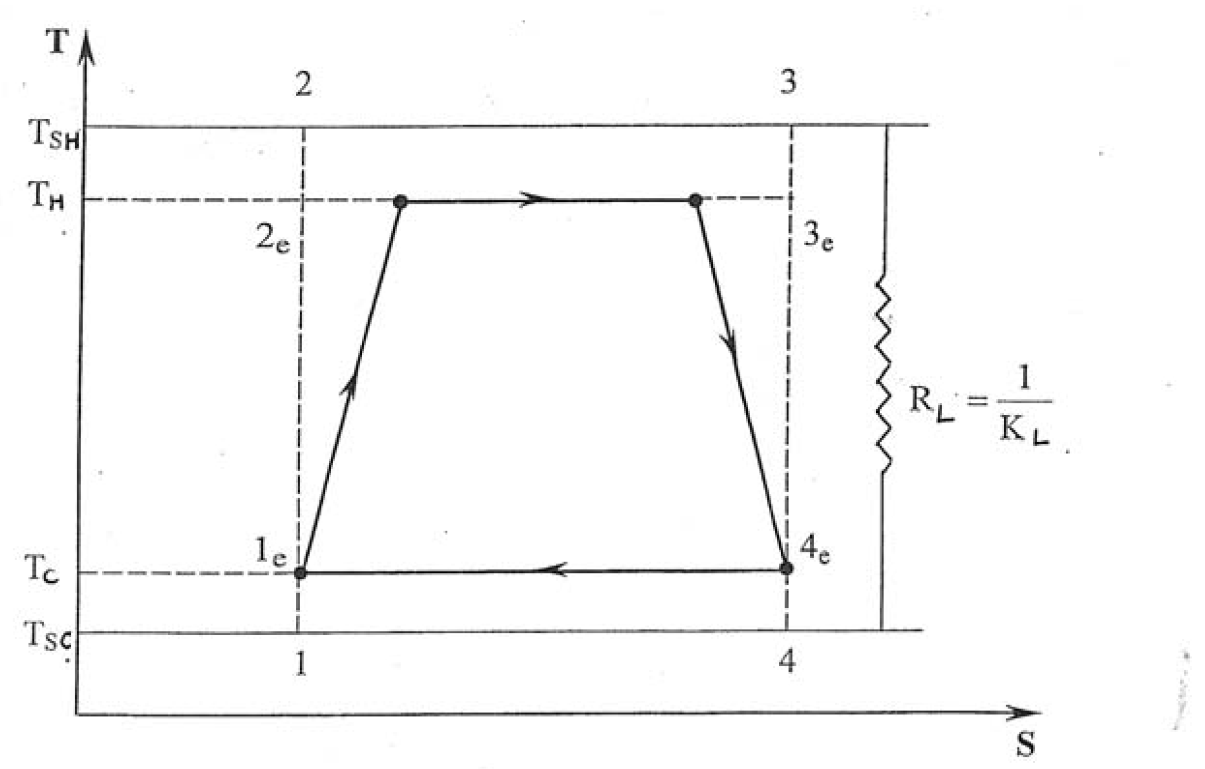
2. The Model: from the Carnot Cycle to the Carnot Heat Engine

We studied the cycle as applied to a Carnot heat engine in contact with two isotherms (a hot at T_SH temperature and a cold isotherm with T_SC temperature). The system (engine and heat reservoirs) is non-adiabatic and thermal losses occur through thermal resistance R_L. The four thermodynamical transformations are linearized and assumed to be irreversible (Figure 1). Internal irreversibility is represented by ${\dot{s}}_i$ that is to say the entropy flux generated inside the functioning in a steady state.

It is well known that the first law efficiency of the Carnot heat engine in the thermostatics limit (equilibrium) is [26]:

$${\eta }_c=1-\frac{T_{SC}}{T_{SH}}$$

(1)

The Chambadal-Novikov-Curzon-Ahlborn efficiency [28] differs from that given by Equation (1) and corresponds to the maximum engine power delivered according to the endoreversible cycle (1e 2e 3e 4e), the external irreversibilities being associated to temperature gradients between engine and reservoirs:

$${\eta }_e(MAX\dot{w})=1-\sqrt{\frac{T_{SC}}{T_{SH}}}$$

(2)

It is thus of interest to show the evolution of the steady state endoreversible engine power versus the consumed energy flux graphically (see Figure 2)

Figure 2. The mean power of an endoreversible CARNOT engine in relation to the heat flux consumed.

Figure 2. The mean power of an endoreversible CARNOT engine in relation to the heat flux consumed.

This figure clearly shows the most efficient zone for the engine on the curve as lying between points 0 and A. Moreover, maximum efficiency occurs at point 0 but with zero power which means that the most efficient point for the engine must be located near to and on the left of point A. This could be presented differently [28] by showing engine power versus efficiency (see Figure 3a).

Figure 3. a). Variation of the Carnot. b). Variation of the Carnot endoreversible engine power versus efficiency, efficiency in presence of thermal losses.

Figure 3. a). Variation of the Carnot. b). Variation of the Carnot endoreversible engine power versus efficiency, efficiency in presence of thermal losses.

If thermal losses (through the engine body at least) are calculated then this is reflected by the differences between Figure 3a and Figure 3b (an endoreversible engine in the presence of heat losses). The presence of engine non-adiabaticity imposes a new value for maximum efficiency $MAX\eta$ at point C; this value is smaller than ${\eta }_C$ and the corresponding high-efficiency zone for the engine is reduced to the interval AC. The same consequences were observed when we studied an endoirreversible engine [20].

3. Entropy Generated versus Irreversibility Ratio

3.1. Irreversibility ratio method

The most commonly-used way to account for the internal irreversibility of a machine (converter) is to introduce a cycle irreversibility ratio I according to [31] :

$$I\frac{{\dot{q}}_H}{T_H}+\frac{{\dot{q}}_C}{T_C}=0$$

(3)

Note : we use here typographical conventions such that ${\dot{q}}_H>0,{\dot{q}}_C<0,\dot{w}>0$, in equations etc.

In this case the corresponding efficiency at maximum power is given by:

$${\eta }_I(MAX\dot{w})=1-\sqrt{I\frac{T_{SC}}{T_{SH}}}$$

(4)

The same methodology applied to a non-adiabatic endoreversible engine gives:

$${\eta }_I(MAX\dot{w})=1{\left[1-\sqrt{\frac{T_{SC}}{T_{SH}}}\right]}^2·{\left[1+\frac{K_L}{K_{eq}}{\eta }_C-\sqrt{\frac{T_{SC}}{T_{SH}}}\right]}^{-1}$$

(5)

with $\frac{1}{K_{eq}}=\frac{1}{K_H}+\frac{1}{K_C}$.

We propose to complete this model by simultaneously considering internal irreversibility and non-adiabaticity whilst bearing in mind that the flux delivered at the hot side $\dot{q}$ remains limited, whatever the source of energy (solar energy, or combustion for example). This differs from some results obtained by previous works on the subject [30] where the thermal capacity of the source, represented by ${\dot{C}}_H={\dot{m}}_H{C}_H$ was finite. The thermal balance at the hot side gives:

$${\dot{q}}_H=K_H(T_{SH}-T_H)=\dot{q}-K_L(T_{SH}-T_{SC})$$

(6)

The corresponding definition of the “stagnation temperature” of the system, T_S (maximum possible temperature of the system) results from ${\dot{q}}_H=0$ as:

$$T_S=\frac{\dot{q}+K_L{T}_{SC}}{K_L}$$

(7)

Engine power is optimized using the same methodology with respect to T_SH variable which gives:

$$MAX\dot{w}=\frac{K_L}{k^{\prime }+1}{(\sqrt{T_S}-\sqrt{I{T}_{SC}})}^2$$

(8)

with $k^{\prime }=\frac{K_L}{K_{eq}^{\prime }};\frac{1}{K_{eq}^{\prime }}=\frac{1}{K_H}+\frac{I}{K_C}$.

$$\eta (MAX\dot{w})=\frac{1}{1+k^{\prime }}\frac{{(\sqrt{T_S}-\sqrt{I{T}_{SC}})}^2}{T_S-T_{SC}}$$

(9)

When I increases, efficiency diminishes. Equation (9) implies that internal irreversibilities are linked to non-adiabaticity (first term of Equation (9)). A maximum of $MAX\dot{w}$ noted $MAX{\dot{w}}_{opt}$ could be obtained for a specific allocation of conductances if the total conductance remains finished (and imposed):

K_T = K_H + K_C

(10)

Thus K_Copt can be expressed as:

$$K_{Copt}=\frac{K_T\sqrt{I}}{1+\sqrt{I}}$$

(11)

and for $\eta (MAX{\dot{w}}_{opt})$:

$$\eta (MAX{\dot{w}}_{opt}) = \frac{1}{1+\frac{K_L}{K_T}(1+{\sqrt{I)}}^2}\frac{{(\sqrt{T_S}-\sqrt{I{T}_{SC}})}^2}{T_S-T_{SC}}$$

(12)

3.2. Generated entropy flux method

In this case, the entropy balance for the engine can be expressed as:

$$\frac{{\dot{q}}_H}{T_H}+\frac{{\dot{q}}_C}{T_C}+{\dot{s}}_i=0$$

(13)

This could be completed by the entropy balance of the whole system (including source and sink) with the total entropy flux ${\dot{s}}_t$ expressed as:

$$\frac{{\dot{q}}_H}{T_{SH}}+\frac{{\dot{q}}_C}{T_{SC}}+{\dot{s}}_t=0$$

(14)

The difference between Equations (14) and (13) confirms that the total entropy flux consists of an internal entropy flux and two external entropy fluxes associated with heat transfer.

Following these calculations:

$$MAX\dot{w}=\frac{K_L}{1-{\dot{s}}_i/K_C+K_L/K_{eq}^{″}}{\left(\sqrt{T_S\left(1-{\dot{s}}_i/K_C\right)}-\sqrt{T_{SC}}\right)}^2$$

(15)

$K_{eq}^{″}$ can be expressed as follows: $\frac{1}{K_{eq}^{″}}=\frac{1}{K_H}+\frac{1}{K_C}-\frac{{\dot{s}}_i}{K_C{K}_H}$.

The maximum of $MAX\dot{w}$ corresponding to a specific allocation of conductances satisfying the limitation of Equation (10) can be expressed as:

$$MAX{\dot{w}}_{opt}=\frac{K_L\left(\sqrt{T_S}-\sqrt{T_{SC}}\right)}{1-{\dot{s}}_i/K_T+4K_L/K_T}\left[\left(\sqrt{T_S}-\sqrt{T_{SC}}\right)\left(1-\frac{{\dot{s}}_i}{K_T}\frac{\sqrt{T_S}+\sqrt{T_{SC}}}{\sqrt{T_S}-\sqrt{T_{SC}}}\right)-\frac{{\dot{s}}_i}{K_L}\frac{T_{SC}}{\sqrt{T_S}-\sqrt{T_{SC}}}\right]$$

(16)

K_Copt can be expressed as:

$$K_{Copt}=\frac{K_T}{2}\frac{1+{\dot{s}}_i\left(\frac{1}{K_L}·\frac{\sqrt{T_{SC}}}{\sqrt{T_S}-\sqrt{T_{SC}}}+\frac{1}{K_T}\frac{\sqrt{T_S}+\sqrt{T_{SC}}}{\sqrt{T_S}-\sqrt{T_{SC}}}\right)}{1+\frac{{\dot{s}}_i}{2K_L}·\frac{\sqrt{T_{SC}}}{\sqrt{T_S}-\sqrt{T_{SC}}}}$$

(17)

for $\eta (MAX{\dot{w}}_{opt}$), the efficiency at $MAX{\dot{w}}_{opt}$ it corresponds to:

$$\eta \left(MAX{\dot{w}}_{opt}\right)=\frac{1}{1-\frac{{\dot{s}}_i}{K_T}+4\frac{K_L}{K_T}}\left[\frac{\sqrt{T_S}-\sqrt{T_{SC}}}{\sqrt{T_S}+\sqrt{T_{SC}}}-{\dot{s}}_i\left[\frac{1}{K_T}·\frac{\sqrt{T_S}+\sqrt{T_{SC}}}{\sqrt{T_S}-\sqrt{T_{SC}}}+\frac{1}{K_L}·\frac{T_{SC}}{T_S-T_{SC}}\right]\right]$$

(18)

3.3. A partial conclusion

As a partial conclusion, the comparison of the two methods is consistent since the same endoreversible limit is used but whilst the ratio method may appear simpler (for example Equation (12) as compared to Equation(18)), the entropy flux method is definitively recommended because it is based on physical laws and entropy analysis [8] gives direct access to ${\dot{s}}_i$ (entropy balance) which appears as a complex function of system variables and parameters. It also allows us to show that the equipartition theorem [32] is only applicable to the allocation of system conductances if the converter is endoreversible (17). It should also be noted that the cold conductance of the engine is greater than the hot conductance at optimum power.

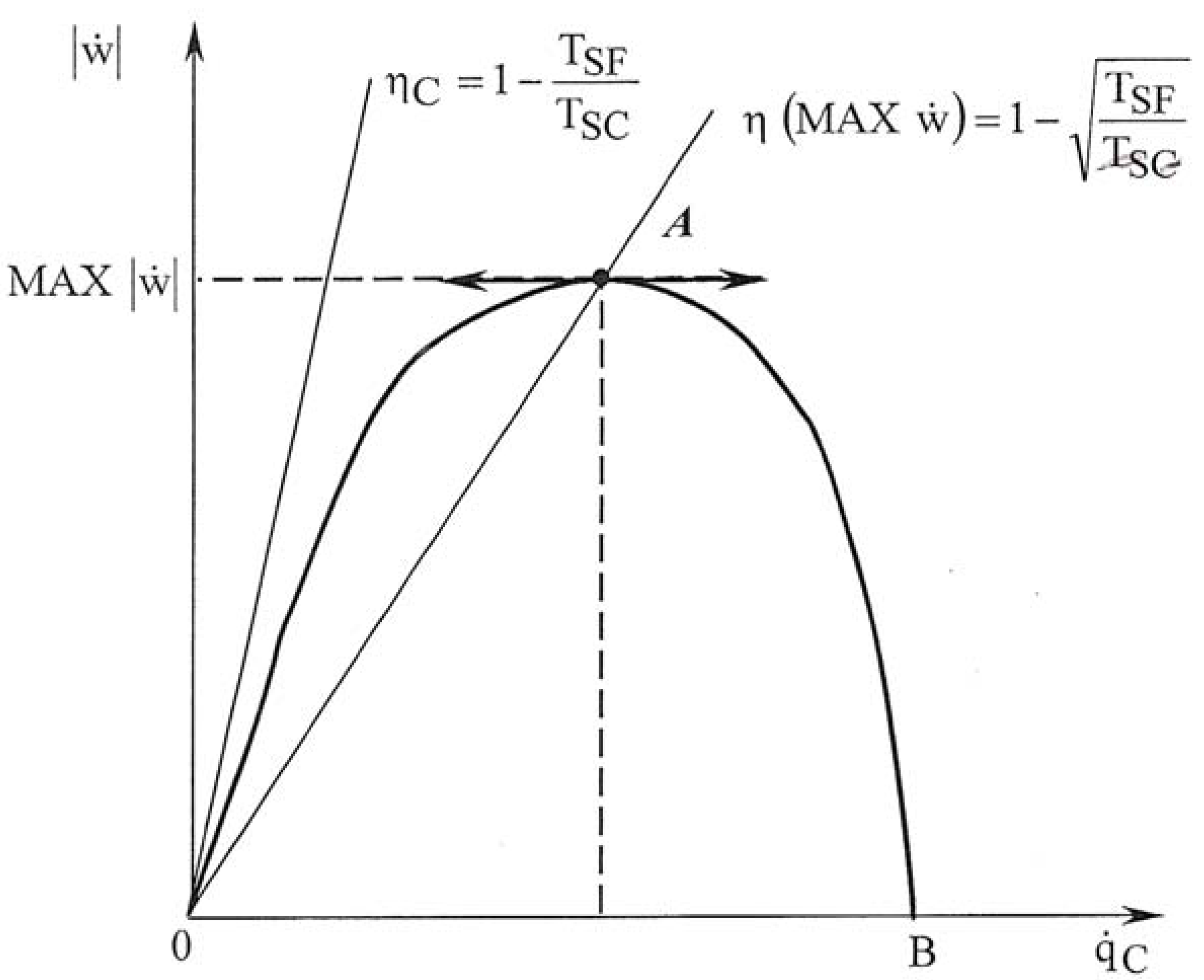
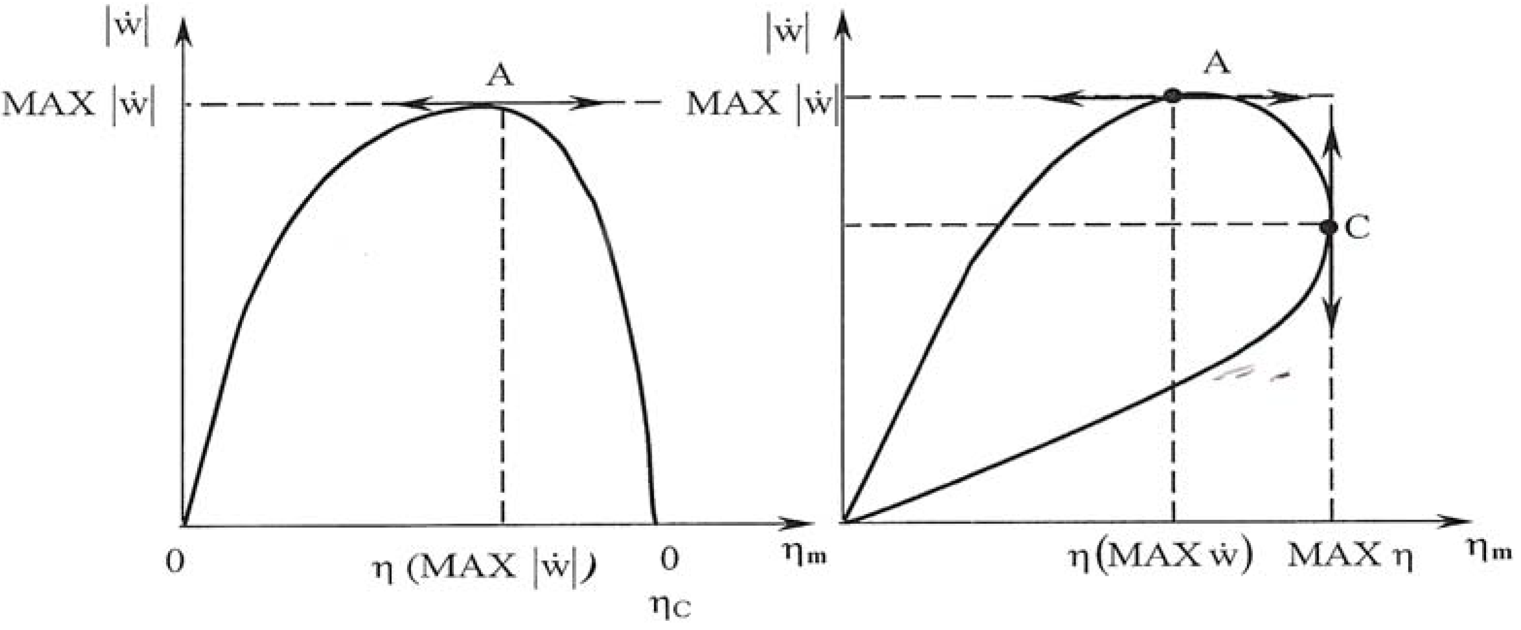
4. Various Optimization Objectives

The main objective functions of every kind of machines (engines, refrigerators, heat pumps…) are useful effect (U.E.), energy consumption (E.C.), and efficiencies. Nowadays it is important to add the release of by-products into the environment, R, to those functions. So the objective functions that require optimization are: MAX [U.E.]; min [E.C.]; min [R]; MAX [efficiencies]. The three first items are linked to the system size while the last function one is non-dimensional and possesses various definitions. The most widely used function was defined in Section 2 and Section 3 of this paper and is relative to the first law of thermodynamics ${\eta }_I$:

$${\eta }_I=\frac{\left|U.E.\right|}{E.C.}$$

(19)

The efficiency factor can be applied to the converter and the corresponding efficiency is a conversion efficiency ${\eta }_{C0}$. It could also be applied to transfer efficiency ${\eta }_{TR}$. If we consider the system as a whole (the converter in its environment) this gives an overall efficiency factor like those discussed in Section 2 and Section 3.

By combining the first and second laws of thermodynamics (which depends on the chosen form of the second law (either Equation (13) or Equation (14)), a general definition of the exergy efficiency ${\eta }_x$ applied to the machine or to the system (machine in its environment) is obtained:

$${\eta }_x=\frac{\left|U.E_x\right|}{E_x.C.}$$

(20)

U.E_x, useful exergy.

E_x.C., exergy consumption or consumed exergy.

Care should be taken to distinguish this definition from the definition given by Grassmann [33].

It should also be noted that the engineering approach is influenced by economics and thus the following objective functions need to be considered-min investment cost and min overall cost (including operating cost which could also be an objective in itself).

This is therefore a question of thermoeconomics.

The influence of the choice of objective functions will be discussed in Section 6 and Section 7, but need to be mitigated due to constraints.

5. Engine Optimization with Constraints

5.1. Model equations

Whatever the problem to be solved, physical equations (the first and second laws of thermodynamics, state equation relative to cycled medium, kinetic equations) represent analytical constraints existing between system variables and parameters.

5.2. Added constraints

There are other constraints added because of physical or engineering limitations. These could include finite size (like Equation (10)), finite time (duration), finite speed, material constraints (maximum pressure or temperature) and finite costs. Environmental and societal constraints are of course growing in importance in today’s world.

This means that Finite Dimensions (size and time) Thermodynamics is now a mandatory subject for the purposes of machine optimization. We will also give examples in the framework of F.D.O.T. (Finite Dimensions Optimal Thermodynamics) of certain cases where other added constraints exist such as imposed power, imposed heat flux input, imposed engine efficiency or limitation relative to temperature (intensive variable) as was discussed in Section 3 (see also [34,35]).

6. The Case of a Combined Heat and Power System (C.H.P.)

6.1. Comparison of the two irreversibility methods

Here we studied a non-adiabatic CARNOT heat engine using the same hypothesis as in Section 3 except for the fact that T_SC now corresponds to a useful temperature level T_u. For hot heat cogeneration T_u > T₀ the ambient temperature (reference temperature).

We used the same mathematical methods as in Section 3.1., but applied them to a new objective function, maximum useful exergy flux $\dot{E}{x}_u$. With heat reference relative to the useful medium (T_u), this can be expressed as follows according to the irreversibility ratio method:

$$\left|\dot{E}{x}_u\right|={\dot{q}}_H\left(1-I\frac{T_0{T}_C}{T_u{T}_H}\right)$$

(21)

More precisely, Equation (21) can be expressed as:

$$\left|\dot{E}{x}_u\right|=K_L\left(T_S-T_{SH}\right)\left(1-\frac{T_0}{T_{SH}(1+k^{\prime })-T_S{k}^{\prime }}\right)$$

(22)

After optimization using the ratio method this gives:

$$MAX{\left|\dot{E}{x}_u\right|}_{opt}=\frac{K_L{\left(\sqrt{T_S}-\sqrt{I{T}_0}\right)}^2}{1+\frac{K_L}{K_T}{\left(1+\sqrt{I}\right)}^2}$$

(23)

$$\eta \left[MAX{\left|\dot{E}{x}_u\right|}_{opt}\right]=\frac{1}{1+\frac{K_L}{K_T}{\left(1+\sqrt{I}\right)}^2}·\frac{{\left(\sqrt{T_S}-\sqrt{I{T}_0}\right)}^2}{T_S-T_0}$$

(24)

A comparison of Equations (24) and (12) shows that if we move from mechanical power optimization to exergy flux optimization, T_SC is replaced by the ambient temperature T₀, and T_u the temperature level of the useful heat does not influence the optimum and the corresponding ${\eta }_I$ efficiency.

Corresponding results are obtained analytically with entropy analysis, when the ${\dot{s}}_i$ parameter is assumed to be constant:

$$\left|\dot{E}{x}_u\right|={\dot{q}}_H\left(1-\frac{T_0{T}_C}{T_u{T}_H}\right)-\frac{T_0{T}_C}{T_u}{\dot{s}}_i$$

(25)

After optimization, with the entropy flux method this gives :

$$MAX{\left|\dot{E}{x}_u\right|}_{opt}=\frac{K_L\left(\sqrt{T_S}-\sqrt{T_0}\right)\left[K_T\left(\sqrt{T_S}-\sqrt{T_0}\right)-{\dot{s}}_i\left(\sqrt{T_S}+\sqrt{T_0}\right)\right]}{K_T-{\dot{s}}_i+4K_L}$$

(26)

Supposing there is always incoming energy flux pure exergy (radiative energy for a solar heating system, or chemical energy for an engine) this corresponds to:

$$\eta \left[MAX{\left|\dot{E}{x}_u\right|}_{opt}\right]=\frac{1}{\sqrt{T_S}+\sqrt{T_0}}·\frac{K_T\left(\sqrt{T_S}-\sqrt{T_0}\right)-{\dot{s}}_i\left(\sqrt{T_S}+\sqrt{T_0}\right)}{K_T-{\dot{s}}_i+4K_L}$$

(27)

Note: these results could be reconsidered in term of efficiencies if we suppose that the incoming energy in the system is converted irreversibly at the contact of the source (radiative to thermal energy for the solar heating system; chemical to thermal energy during combustion for an internal combustion engine).

In the case of a solar heating system the input exergy flux is:

$$\dot{E}{x}_C=K_L\left(T_S-T_0\right)\left(1-\frac{T_0}{T_{SH}}\right)$$

(28)

So the corresponding exergy efficiency is expressed as:

$${\eta }_x\left[MAX|\dot{E}{x}_{u_{opt}}\right]=\frac{1}{\sqrt{T_S}+\sqrt{T_0}}·\frac{K_T\left(\sqrt{T_S}-\sqrt{T_0}\right)-{\dot{s}}_i\left(\sqrt{T_S}+\sqrt{T_0}\right)}{K_T-{\dot{s}}_i+4K_L}$$

$$·\frac{\left[\left(K_T+{\dot{s}}_i\right)\sqrt{T_0}+4K_L\sqrt{T_S}\right]\sqrt{T_S}}{K_T\left(\sqrt{T_S}-\sqrt{T_0}\right)\sqrt{T_0}+{\dot{s}}_i\left(\sqrt{T_S}+\sqrt{T_0}\right)\sqrt{T_S}+4K_L\left(T_S-T_0\right)}$$

(29)

As a partial conclusion, it can be noted that the entropy flux method permits a more precise identification of the influence of internal irreversibility and thermal losses.

6.2. Extension of these results to cases with an extra constraint

The synthesis of the optimization results for an adiabatic engine when the objective function O.F. is the efficiency ${\eta }_I$, respectively the power $\dot{w}$, or the energy consumption ${\dot{q}}_H$, was reported in a recent paper [14].

The same development has been applied to reverse cycle machines (submitted for publication). For the purposes of this study our intention was to extend these results to the Carnot C.H.P. system considering the useful exergy $\dot{E}{x}_u$ to be the objective function but with various added constraints representative of hot combined heat and power systems. We mainly obtained simple analytical results except when $\dot{w}={\dot{w}}_0$, the mechanical power imposed (a second order equation needs to be solved).

Table 1 summarizes the results obtained for MAX (−Ex_u), the useful exergy flux when the irreversibility ratio method is used. The optimum of this objective function corresponds to the case without constraint:

$$MAX\left(-\dot{E}{x}_u\right)=\frac{K_T{K}_L}{K_T+4K_L{\left(1+\sqrt{I}\right)}^2}{\left(\sqrt{T_S}-\sqrt{I{T}_0}\right)}^2$$

(30)

The results in the endoreversible case are straightforward.

Table 1. Constrained optimum for a CARNOT CHP system irreversible ratio method.

	O.F.	MAX ($\dot{E}{x}_u$)
Added constraint
R = $\frac{{\dot{q}}_u}{{\dot{w}}_0}=$R0		$\frac{K_T{K}_L}{K_T+K_L{\left(1+\sqrt{I}\right)}^2}\left(T_S-I\frac{1+R_0}{R_0}\right)\left(1-\frac{T_0}{T_u}·\frac{R_0}{1+R_0}\right)$
$\dot{w}={\dot{w}}_0$
${\dot{q}}_u={\dot{q}}_0$		$\frac{K_T{K}_L{T}_S}{K_T+K_L\left[{\left(1+\sqrt{I}\right)}^2-\frac{I{K}_T{T}_u}{{\dot{q}}_0}\right]}+\frac{K_T{T}_0}{K_T{T}_u}{\dot{q}}_0$
without		$\frac{K_T{K}_L}{K_T+K_L{\left(1+\sqrt{I}\right)}^2}{\left(\sqrt{T_S}-\sqrt{I{T}_0}\right)}^2$

Table 1. Constrained optimum for a CARNOT CHP system irreversible ratio method.

	O.F.	MAX ($\dot{E}{x}_u$)
Added constraint
R = $\frac{{\dot{q}}_u}{{\dot{w}}_0}=$R0		$\frac{K_T{K}_L}{K_T+K_L{\left(1+\sqrt{I}\right)}^2}\left(T_S-I\frac{1+R_0}{R_0}\right)\left(1-\frac{T_0}{T_u}·\frac{R_0}{1+R_0}\right)$
$\dot{w}={\dot{w}}_0$
${\dot{q}}_u={\dot{q}}_0$		$\frac{K_T{K}_L{T}_S}{K_T+K_L\left[{\left(1+\sqrt{I}\right)}^2-\frac{I{K}_T{T}_u}{{\dot{q}}_0}\right]}+\frac{K_T{T}_0}{K_T{T}_u}{\dot{q}}_0$
without		$\frac{K_T{K}_L}{K_T+K_L{\left(1+\sqrt{I}\right)}^2}{\left(\sqrt{T_S}-\sqrt{I{T}_0}\right)}^2$

A third optimization calculation could be performed by finding the best allocation between thermal losses (K_L) and the total heat conductance K_T of the thermomechanical system. Supposing we dispose of K = K_L + K_T to allocate, with the same value for K_L and K_T, this can be expressed as:

$$OPT\left[MAX\left(\dot{E}{x}_u\right)\right]=\frac{K}{10}{\left(\sqrt{T_S}-\sqrt{T_0}\right)}^2$$

(31)

Even if this result may not be a highly accurate approximation, it does show a new optimization allocation between heat loss and heat transfer conductances. This approach would need to be refined using thermoeconomics but nevertheless represents the best compromise between heat transfers from the source sinking through the engine and thermal losses (insulation conductance ).

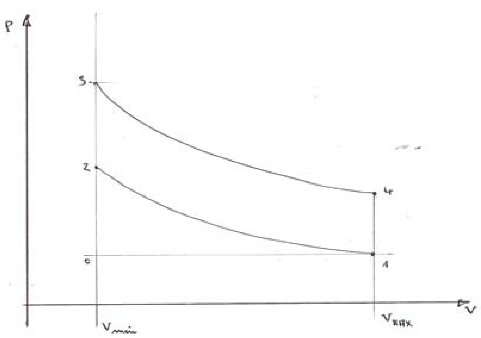
7. The Case of the Internal Combustion Engine (I.C.E.)

Here we study the example of an engine working on the basis of the OTTO (BEAU DE ROCHAS) cycle (Figure 4). The revisited model is based on the two laws of thermodyamics. The first law applied to the cycled gas is:

$$W+C_V\left(T_3-T_2\right)+C_V\left(T_1-T_4\right)=0$$

(32)

This equation is written with reference to the cycled gas mass $\dot{M}$ with the cycled gas assumed to be a perfect gas.

Figure 4. Representation of the OTTO Cycle engine in the CLAPEYRON diagram.

Figure 4. Representation of the OTTO Cycle engine in the CLAPEYRON diagram.

We add the energy balance corresponding to the heat release to Equation (32):

$$q=\frac{\dot{m}LHV}{\dot{M}}=C_V\left(T_3-T_2\right)+k_L\left(\frac{T_3+T_2}{2}-T_w\right)$$

(33)

$\dot{m}$, fuel mass flux

LHV, low heating value of the fuel

$k_L=\frac{K_L}{\dot{M}}$, heat loss coefficient during combustion

T_w, cylinder wall temperature.

We presume that heat loss mainly occurs during the combustion process (as has been noted in some previous studies), that is to say via adiabatic compression and expansion.

The second law using the entropy flux method gives the entropy balance applied to the cycled gas as:

$$\dot{M}{C}_V\left[\ln \frac{T_3}{T_2}+\ln \frac{T_1}{T_4}\right]+{\dot{s}}_i=0$$

(34)

${\dot{s}}_i$, supposed constant is the entropy flux created in the gas during the whole cycle resulting from solid and fluid irreversibilities on the gas. Equation (34) is thus re-calculated as follows:

$$\frac{T_3{T}_1}{T_2{T}_4}=K=e^{-{\dot{s}}_i/\dot{M}{C}_V}$$

(35)

7.1. The incoming energy flux (fuel consumption) is imposed

If $\dot{m}/\dot{M}$ is imposed, q results as a parameter through Equation (33).

The objective function is the useful effect W (32) and the variable temperatures T₂, T₃, T₄ are subject to the two physical constraints (Equations 33, 35).

The results of optimization in term of $T_{2_{opt}}$, representative of the associated optimum volumetric ratio $r_{V_{opt}}$ can easily be expressed analytically as follows:

$$r_{V_{opt}}=\frac{VMAX}{V\min }={}^{\gamma -1}\sqrt{T_{2_{opt}}/T_1}$$

(36)

$$T_{2_{opt}}=a{T}_{1}witha=\sqrt{\frac{q+k_L{T}_W}{k_L{T}_1}·\frac{1}{K}}=\sqrt{\frac{Tad}{K{T}_1}}$$

$$MAX\left(-W)\right)=C_V{T}_1\left\{a\left[aK\left(1-\alpha \right)+\alpha \right]\left(1-\frac{1}{aK}\right)+1-a\right\}$$

(37)

with $\alpha =\frac{C_V-k_L/2}{C_V+k_L/2}$

7.2. An engine with imposed maximum temperature T_MAX

Generally the thermomechanical material limitation appears to be the dominant constraint which imposes a maximum temperature limitation on the burned gas, T_MAX = T₃.

It results in a corresponding heat release:

$$q=\left(C_V+\frac{k_L}{2}\right)T_{MAX}-k_L{T}_W-\left(C_V-\frac{k_L}{2}\right)T_2$$

(38)

Combining equations (32) and (35) gives the following:

$$W=-C_V\left[T_{MAX}-T_2-\frac{T_{MAX}{T}_1}{K{T}_2}+T_1\right]$$

(39)

It is easy to deduce that the optimum of W is obtained for $T_{2_{opt}}^{\prime }=\sqrt{\frac{T_{MAX}{T}_1}{K}}$, and:

$$MAX\left(-W\right)=C_V\left[{\left(\sqrt{T_{MAX}}-\sqrt{\frac{T_1}{K}}\right)}^2+T_1\left(1-\frac{1}{K}\right)\right]$$

(40)

The corresponding ${\eta }_I$ efficiency results from Equations (38) and (40). A new result, the endoreversible limit ( K = 1), is obtained:

$${\eta }_I{\left[MAX\left(-W\right)\right]}_{endo}=\frac{{\left(\sqrt{T_{MAX}}-\sqrt{T_1}\right)}^2}{\sqrt{T_{MAX\text{}}}\left(\sqrt{T_{MAX}}-\sqrt{T_1}\right)+\frac{k_L}{2C_V}\left(T_{MAX}+\sqrt{T_{MAX}{T}_1}-2T_w\right)}$$

(41)

This results could be applied more specifically to an adiabatic engine (k_L = 0). For the first time we obtained, using equation (41), the remarkable result of Chambadal–Novikov–Curzon–Ahlborn [3] applied to an internal combustion engine within the limits of an adiabatic and endoreversible case.

7.3. Further details and results

The search for maximum efficiency could also be performed using temperature limitation (Section 7.2.) as the dominant constraint.

Our aim with this work was to extrapolate from the more basic case to a more elaborated case to highlight the usefulness of the proposed methodology. The basic cases could be kept for tendency and feasibility results whereas the elaborated model could be extremely helpful for sensitivity analysis and so forth albeit with higher modeling and calculation costs.

Details of the internal combustion engine modeling, as well as numerical and computation procedures are given in ref. [36,37]. For the sake of brevity they are briefly summarized hereafter. The kinematics of the piston assembly is described according to the classic model (with $\theta$, crankshaft angular position as variable), the mass balance is determined by noting pressure losses at the intake and exhaust. Mechanical losses due to friction and pumping are calculated using Heywood’s correlation and heat losses through the cylinder are estimated using the Hohenberg correlation.

Figure 5 gives the results obtained using this model. It shows the sensitivity analysis of power versus efficiency for a spark ignition engine, with mean parameter values of V_cyl, cylinder volume, 0, 5 litre, R_SB, stroke to bore ratio, 1, $\epsilon$, volumetric ratio, 16, T_W, cylinder wall temperature, 480 K, $\varphi$, fuel air ratio, 0, 70, and ${\theta }_0$, ignition advance, –5°.

Figure 5. Power versus efficiency curves for an I.C.E.

Figure 5. Power versus efficiency curves for an I.C.E.

Figure 5a reports the sensitivity to $\epsilon$, Figure 5b respectively to ${\theta }_0$, Figure 5c to R_SB and Figure 5d, to V_cyl. A maximum power point and a maximum efficiency point can be noted on each figure. Each of these points is associated with a given angular speed of the engine and the optimal zone for the engine is in between.

An increase in $\epsilon$, or a decrease in ${\theta }_0$ is favourable in terms of obtaining maximum power and efficiency. The last two parameters tend to have more contrasting influences. An increase in the R_SB ratio has a large negative influence on power but leads to a less pronounced increase in efficiency (Figure 5c). An increase in cylinder volume has a medium negative influence on specific volumetric power but a significant positive influence on efficiency (Figure 5d). These results should be interpreted in light of current engine tendencies (dow sizing) and complementary constraints (practical limitations) should also be borne in mind. Complements to the model are currently being developed.

8. Conclusions

8.1. The present paper features a short overview of thermodynamics from Carnot to the present

First the paper focused on model evolution from the Carnot cycle to the Carnot engine. We put particular emphasis on the Carnot heat engine but corresponding results have been developed by the author for reverse cycle Carnot machines [38,39].

8.2. Comparison between the irreversibility ratio and the entropy flux method

For the first time a comparison has been made of the irreversibility ratio method, and the entropy flux method for engines in the presence of heat losses while introducing the concept of limited maximum temperature of the studied system. T_S was named stagnation temperature for a thermomechanical system with heat source and sink which corresponds clearly to the solar heating system. In the case of an internal combustion engine, T_S corresponds to the adiabatic combustion temperature of the flue gas.

The classic maximum power levels of the Carnot engine were compared. The result was the recommendation that the entropy flux method should be used even if calculation may appear a little more complicated due to the fact that ${\dot{s}}_i$ the entropy flux created due to irreversibilities, is undoubtedly a complex physical function that could be obtained through careful entropy analysis or experimental identification.

8.3. New objective functions (energy comsumption, environmental pollution etc)

Until now the main objective function for engines has always been power and also perhaps efficiency. This paper suggests it is necessary to rethink this question and add energy consumption, the release of by-products into the environment to those objective functions. Similarly other efficiency rating than the first law efficiency need to be considered, for example second law efficiencies (the author considers this essential for combined Heat and Power applications: see Section 6). It would also be important to develop thermoeconomical objectives but examples have not been given in this paper.

8.4. New constraints (imposed energy consumption, power, efficiency etc.)

Until now, few research articles have covered other constraints. In this paper we proposed three main cases wherein optimization of the system was carried out with imposed energy consumption (for example using a solar heating system or an internal combustion engine).

This was shown to correspond to temperature limitation (finite temperature). The paper also discussed the case of an engine with an imposed or demanded given power and a second case where the corresponding first law efficiency was imposed (control purpose).

These added constraints clearly seem to have a definite effect on optimum factors. Clear illustration of this was given in the reported example of a Carnot C.H.P. system Table 1) where the objective function was the optimum of useful exergy flux.

8.5. Enlarged concept of F.D.O.T.

The present research has also been developed further for a gas turbine [35] and for the Stirling engine [40]. Hopefully the models will continue to be improved in the near future with the joint aim of developing the frame of Finite Dimensions Optimal Thermodynamics methodology (F.D.O.T.) and continuing to validate the proposed model by comparison with experimental results as was recently the case for refrigerating machines [38].

References

1. Maury, J.P. Carnot et la machine à vapeur; P.U.F.: Paris, France, 1987. [Google Scholar]
2. Onsager, L. Reciprocal relations in irreversible processes I. Phys. Rev. 1931, 37, 405. [Google Scholar]Reciprocal relations in irreversible processes II. Phys. Rev. 1931, 38, 2265. [CrossRef]
3. Curzon, F.L.; Ahlborn, B. Efficiency of a Carnot engine at maximum power output. Am. J. Phys. 1975, 1, 22–24. [Google Scholar] [CrossRef]
4. Feidt, M. Thermodynamique et optimisation énergétique des systèmes et procédés; TEC et DOC: 2ème édition Paris, France, 1996; p. 343. [Google Scholar]
5. Chambadal, P. Les centrales nucléaires; A. Colin: Paris, France, 1957. [Google Scholar]Le choix du cycle thermique dans une usine génératrice nucléaire; Revue Générale d'Electricité, 1958.Evolution et applications du concept d'entropie; Dunod: Paris, France, 1963; p. 84.
6. Novikov, I. The efficiency of atomic power stations (a review). Atomaya Energiya 1957, 3–11. [Google Scholar] [CrossRef]
7. Kondepudi, D.; Prigogine, I. Modern Thermodynamics; Wiley: Chicester, UK, 1998. [Google Scholar]
8. Bejan, A. Entropy generation minimization : the new thermodynamics of finite size and finite time processes. J. Appl. Phys. 1997, 79, 1191–1218. [Google Scholar] [CrossRef]
9. Chen, L.; Wu, C.; Sun, F. Finite time thermodynamic optimization or entropy generation minimization of energy system. J. Non Equil. Thermodyn. 1999, 24, 327–359. [Google Scholar] [CrossRef]
10. Ourmayaz, A.; Sogut, S.O.; Sahin, B.; Yavuz, H. Optimization of thermal systems based on finite time thermodynamics and thermoeconomics. Prog. Energ. Combust. Sci. 2004, 30, 175–217. [Google Scholar] [CrossRef]
11. Wu, C.; Kiang, R.L.; Lopardo, V.J.; Karpouzian, G.N. Finite time thermodynamics and endoreversible heat engines. Int. J. Mech. Eng. Edu. 1993, 21, 337–346. [Google Scholar] [CrossRef]
12. Salomon, P.; Nitzan, A. Finite time optimization of a newton's law Carnot cycle. J. Chem. Phys 1981, 74, 3546–3560. [Google Scholar] [CrossRef]
13. Salomon, P.; Andresen, B.; Berry, R.S. Thermodynamics in finite time II. Potentials for finite time processes. Phys. Rev. A 1977, 15, 2094–2102. [Google Scholar] [CrossRef]
14. Feidt, M. Optimal use of energy systems and processes. Int. J. Exergy. (in press). [CrossRef]
15. Gutkowicz-Krusin, D.; Procaccia, I.; Ross, J. On the efficiency of rate processes. Power and efficiency of heat engines. J. Chem. Phys. 1978, 69, 3898–3906. [Google Scholar] [CrossRef]
16. Stitou, D.; Feidt, M. Nouveaux critères pour l'optimisation et la caractérisation des procédés thermiques de conversion énergétique. Int. J. Therm. Sci. 2005, 44, 1142–1153. [Google Scholar] [CrossRef]
17. Andresen, B.; Salamon, R.; Berry, R.S. Thermodynamics in finite time : extremals for imperfect heat engines. J. Chem. Phys. 1977, 66, 1571–1577. [Google Scholar] [CrossRef]
18. Patria, R.K.; Nulton, J.D.; Salamon, P. Carnot like processes in finite time II. Applications to model cycles. Am. J. Phys. 1993, 61, 916–924. [Google Scholar] [CrossRef]
19. Gordon, J.M.; Huleilil, M. General performance characteristics of real heat engines. J. Appl. Phys. 1992, 7, 829–837. [Google Scholar] [CrossRef]
20. Petre, C.; Costea, M.; Petre, C.; Petrescu, S. Optimization of the direct Carnot cycle. Appl. Therm. Eng. 2007, 27, 829–839. [Google Scholar]
21. Wu, C.; Kiang, R.L. Finite time thermodynamic analysis of a Carnot engine with internal irreversibility. Energy 1992, 1, 1173–1178. [Google Scholar] [CrossRef]
22. Feidt, M. Thermodynamics and optimization of reverse cycle machines, in Thermodynamics Optimization of Complex Energy Systems; Kluwer Academic Publishers: Morwell, MA, USA, 1999. [Google Scholar]
23. Feidt, M.; Philippi, I. Basis of a general approach for finite time Thermodynamics applied to two heat reservoirs machine. In Int. Symposium ECOS'92, Zaragosa, Spain; 1992. [Google Scholar]
24. Feidt, M. Thermodynamique en temps fini des cycles moteurs ou générateur de froid ou de chaud. In Invited Lecture at the Second Conference of Romanian Society of Thermotechnics, Bucuresti, Romania; 1993. [Google Scholar]
25. Feidt, M.; Ramany-Bala, P.; Benelmir, R. Synthesis, unification and generalization of preceding finite time studies devoted to Carnot cycles; Flowers: Firenze, Italy, 1994. [Google Scholar]
26. Goth, Y.; Feidt, M. Recherches des conditions optimales de fonctionnement des pompes à chaleur ou machines à froid associées à un cycle de Carnot endoreversible. C.R. Acad. Sc.: Paris, France, 1986; 303 Série II–1; pp. 113–122. [Google Scholar]
27. Feidt, M. Optimization of thermal systems and processes, applications to heat pump. In ICIAM'87, Paris, France; 1987. [Google Scholar]
28. Feidt, M.; Petrescu, S.; Costéa, M. Du rendement de Carnot à la Thermodynamique en Temps Fini.; CFGP: Nancy, France, 2001; pp. 125–133. [Google Scholar]
29. Feidt, M. La Thermodynamique en Temps Fini, Histoire et Avenir. In Conférence invitée séminairede la Chaire de Thermotechnique, Université Polytechnique de Bucarest, Romania; 2003. [Google Scholar]
30. Chen, J.; Yan, Z.; Lin, G.; Andresen, B. On the Curzon-Ahlborn efficiency and its connexion with efficiencies of real engines. Energ. Conv. Manage. 2001, 42, 173–181. [Google Scholar] [CrossRef]
31. Ibrahim, O.M.; Klein, S.A.; Mitchell, J.W. Optimum heat power cycles for specified boundary conditions. J. Eng. Gas Turb. Power 1991, 113, 514. [Google Scholar] [CrossRef]
32. Tondeur, D.; Kvaalen, E. Equipartition of entropy production. An optimally criterion for transfer and separation processes. Ind. Chem. Res. 1986, 26, 2827–2833. [Google Scholar]
33. Feidt, M.; Lang, S. Conception optimale de systèmes combinés à génération de puissance, chaleur et froid. Entropie 2002, 242, 2–11. [Google Scholar]
34. Descieux, D.; Feidt, M. Analysis of the non adiabatic Dual cycle at maximum imposed temperature, application to C.H.P. system. In Proceedings ECOS'07, Padova, Italy; 2007; pp. 885–892. [Google Scholar]
35. Feidt, M.; Costea, M.; Postelnicu, V. Comparaison entre le cycle simple de Brayton avec apport thermique imposé et avec contrainte de température maximale. OGST Revue de l'IFP 2006, 61, 237–247. [Google Scholar] [CrossRef]
36. Descieux, D. Modélisations et comparaison énergétique de systèmes de cogénération. Ph.D. Thesis, University Henri Poincaré, Nancy, France, 2007. [Google Scholar]
37. Descieux, D.; Feidt, M. One zone thermodynamic model simulation of an ignition compression engine. Appl. Therm. Eng. 2007, 27, 1457–1466. [Google Scholar] [CrossRef]
38. Feidt, M. Thermodynamics and optimization of reverse cycle machines : refrigeration, heat pump, air conditioning, cryogenics. In thermodynamic optimization of complex energy systems; Kluwer Academic Publishers: Morwell, MA, USA, 1998; pp. 403–410. [Google Scholar]
39. Feidt, M. Advanced Thermodynamics of reverse cycle machine in low temperature and cryogenic refrigeration; Kluwer Academic Publishers: Morwell, MA, USA, 2003; pp. 39–82. [Google Scholar]
40. Petre, C. L'utilisation de la thermodynamique à vitesse finie pour l'étude et l'optimisation de cycle de CARNOT et des machines de STIRLING. Ph.D. Thesis, Universities of Nancy, Nancy, France, 2007. [Google Scholar]