Topdressing Nitrogen Demand Prediction in Rice Crop Using Machine Learning Systems

Abstract

This research is an outcome of the R&D activities of Ecodevelopment S.A. (steadily supported by the Hellenic Agricultural Organization—Demeter) towards offering precision farming services to rice growers. Within this framework, a new methodology for topdressing nitrogen prediction was developed based on machine learning. Nitrogen is a key element in rice culture and its rational management can increase productivity, reduce costs, and prevent environmental impacts. A multi-source, multi-temporal, and multi-scale dataset was collected, including optical and radar imagery, soil data, and yield maps by monitoring a 110 ha pilot rice farm in Thessaloniki Plain, Greece, for four consecutive years. RapidEye imagery underwent image segmentation to delineate management zones (ancillary, visual interpretation of unmanned aerial system scenes was employed, too); Sentinel-1 (SAR) imagery was modelled with Computer Vision to detect inundated fields and (through this) indicate the exact growth stage of the crop; and Sentinel-2 image data were used to map leaf nitrogen concentration (LNC) exactly before topdressing applications. Several machine learning algorithms were configured to predict yield for various nitrogen levels, with the XGBoost model resulting in the highest accuracy. Finally, yield curves were used to select the nitrogen dose maximizing yield, which was thus recommended to the grower. Inundation mapping proved to be critical in the prediction process. Currently, Ecodevelopment S.A. is expanding the application of the new method in different study areas, with a view to further empower its generality and operationality.

1. Introduction

Nitrogen (N) fertilization is by far the most vital input in rice growing for ensuring high yields. Greek growers tend to oversupply with N for acquiring maximum yield, but this results in higher-than-appropriate fertilization costs, high N losses to the environment, increased rice lodging and reduced yield due to spikelet sterility under cool weather conditions [1,2,3]. Moreover, higher N supply than optimum in rice results in denitrification, which converts soil N to N gas—N₂O [2,4]. The resulting atmospheric N oxide is an important greenhouse gas consuming stratospheric ozone [5]. Finally, high N supply can lead to surface runoff as nitrate [6,7].

It is obvious that forecasting precise N-needs before topdressing applications would provide rice growers with a very powerful tool in their attempt to manage nitrogen wisely. In this direction, a common approach is to use rice growth simulation models, such as RiceGrow and ORYZA2000, which can provide insight about rice growth and yield [8,9]. Despite their robust theoretical background to describe rice growth under various conditions, however, these models are difficult to be used extensively in routine applications of commercial rice farming because they require high expertise by the users and data that cannot easily be recorded by the growers [8]. As Gomez (2019) [10] suggested, these sophisticated models have many limitations in real-field applications, as the cost for obtaining the necessary input data is high and the quality of the input data under the commercial practice is obviously compromised.

An alternative to complex growth simulation models is data-driven prediction models using machine learning and open-source remote sensing data [10,11] within the framework of precision agriculture. Machine learning is a branch of artificial intelligence (AI) focused on building applications that learn from data and experience, thus improving their accuracy in decision-making capability over time. Artificial Neural Networks (ANN) and Support Vector Machines (SVM) are the most used techniques applied in several experiments conducted in this context [12].

Precision agriculture (or precision farming) aims at providing spatial information enabling growers to make more precise management decisions [12,13]. For example, if nutrient variability within field parcels, along with variation in the physical properties of the soil, are properly detected, this will allow variable treatment applications, optimizing nutrient supply to the crops and maximizing yields. Field parcel segmentation takes place by matching zones within the field having particular requirements with different management treatments [12,14].

Peng et al., (2010) [15] have notified various problems in the adoption of precision agriculture by rice growers, and various solutions have been suggested, such as the development of satellite remote sensing technologies (e.g., canopy reflectance sensors) or satellite monitoring for determining the timing and rate of N topdressing fertilizer during the rice-growing season. Among several image types, the freely available (optical or radar) Sentinel satellite imagery (provided a cloud-free sky for the optical data) can offer the required information on regular 5-day intervals for commercial crop production [10].

In addition to that, with the development of yield mappers mounted on rice harvesters, there is a steady increase in the availability of rice yield data, lately; yield prediction in precision agriculture is a piece of significant information in crop management [16]. It is projected that by applying data-driven models to satellite data, modern agriculture will become a real-time artificial intelligence system, achieving high efficiency in optimizing inputs and increasing yields [17].

Towards offering precision farming services to rice growers, Ecodevelopment S.A. entered the field in 2016, specializing in fertilization applications. The company has been monitoring and consulting about 1500 ha of rice (shared between 15 different farms) throughout Greece all these years, providing vertical precision farming support to the growers (from crop heterogeneity detection, to interpretation, decision-making, and applications). The company is steadily receiving scientific and technical backup by the Soil and Water Resources Institute, Hellenic Agricultural Organization—Demeter (see Aschonitis et al., (2019) [18]).

In this direction, the main aim of this research was to set up a new methodology for predicting topdressing nitrogen demands in rice cultivation from soil and satellite data. Soil data are necessary to provide basic information on soil type and behavior, while satellite data can provide the required near real-time information on rice growth and possible particularities. The amount, type, and distribution of the available dataset allowed the use of machine learning in this attempt. According to our knowledge, machine learning has not been applied with satellite-based remote sensing data for predicting nitrogen topdressing demands in rice up until now. More specific objectives were to:

• Build a Machine Learning System (MLS) for rice yield prediction to select the optimum nitrogen fertilization scheme.
• Develop a Computer Vision algorithm to map inundated rice fields, which, in turn, allows determination of rice growth stage. Getting this important information from satellite data is faster and more secure than querying all the growers of a large rice cultivation area.

2. Study Area

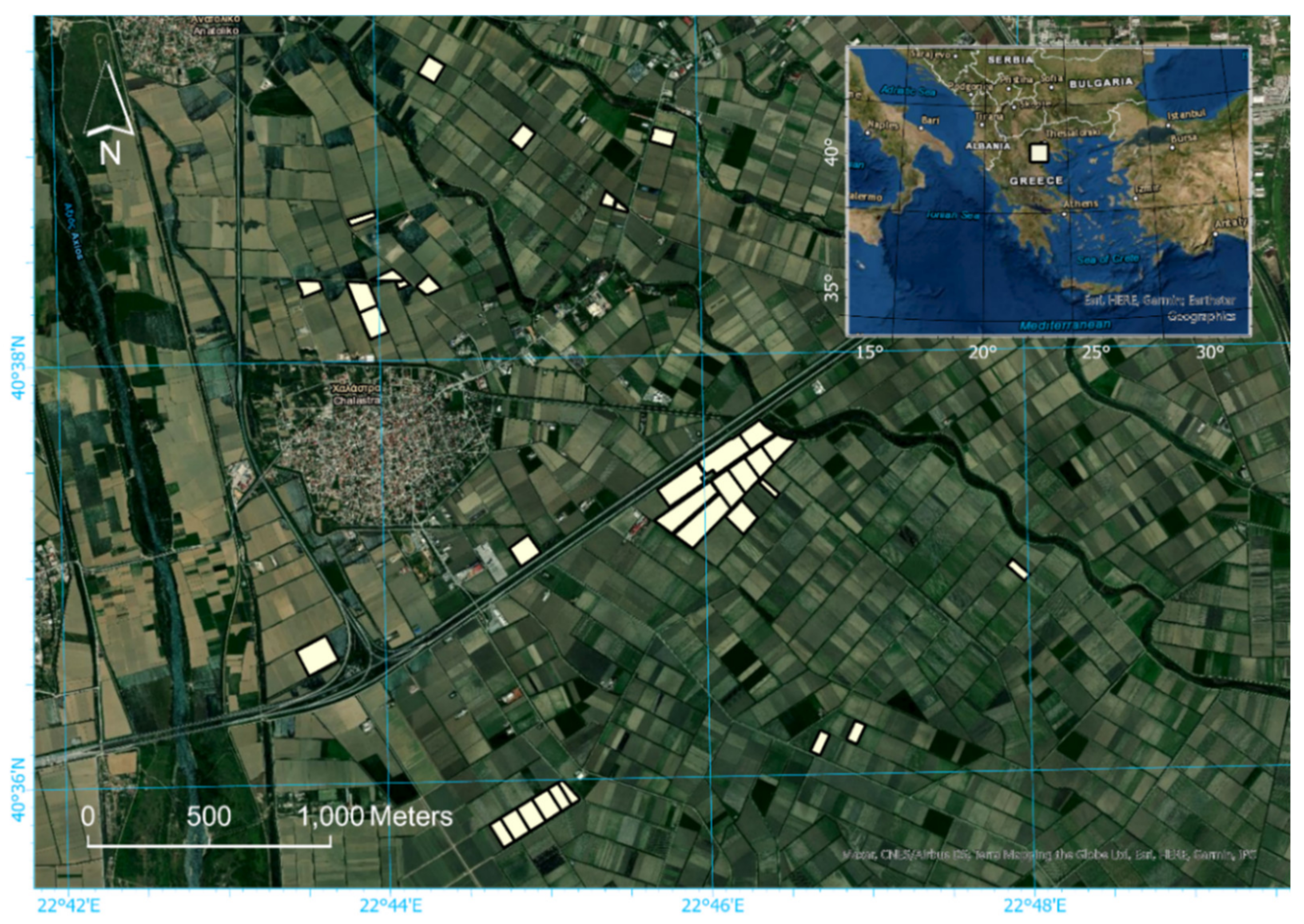
Currently, an extent of 20,000 ha of rice is grown in Thessaloniki Plain. The study area comprises a rice farm in the Plain of Thessaloniki, Greece, within the agricultural area of Chalastra village. A long and a medium grain variety (cv. Thai Bonnet and Ronaldo, respectively) were water-seeded for four consecutive years: 2016, 2017, 2018, and 2019. During the growing season, the grower tried to maintain a 10 cm flood depth. However, fields were drained for a relatively long period of seven days, which is the standard practice for rice growing in Greece, for application of foliar herbicides.

The total extent of the study farm ranged from 99.9 to 128 ha over the monitoring years, averaging to 112.2 ha and shared between 30 rice fields (minimum, in 2019) and 36 rice fields (maximum, in 2016). Differences in farm size and field allocation was due to rotation (mainly with maize), occasional field merging and renting of new land or abandonment of other. However, a major part of the cultivated land was spatially constant over the period (about 90.7 ha) (Figure 1).

The whole management was based on dividing the fields into management zones according to the precision agriculture principles. The management zones were delineated first in 2016 and remained geometrically constant for 2017. In 2018, most of the zones were further divided and remained constant in 2019, too (

Table 1. A summary of the study rice fields and their management zones over the years.

Year	Total Extent (ha)	Number of Fields	Average Field Extent (ha)	Number of Management Zones	Average Extent of Zone (ha)
2016	99.9	36	2.77	55	1.81
2017	107.8	35	3.08	58	1.85
2018	113.0	36	3.13	118	0.95
2019	128.0	30	4.26	118	1.08

).

3. Method Overview

The methodology developed in this research constitutes a precision agriculture approach using machine learning. In machine learning, algorithms are trained to find patterns and features in massive amounts of data to make decisions and predictions based on new data. With precision agriculture, crop fields are divided into management zones, so that variability is minimized within every zone and maximized between them [19].

In this study, management zones were delineated with segmentation of a RapidEye image time-series of year 2015 [15] and ancillary with visual interpretation of unmanned aerial system (UAS) data. The created management zones were used as the spatial units of the machine learning modelling framework.

Then, a representative soil sample was extracted from every zone with soil surveys conducted from 2016 to 2018. The extracts were sent for laboratorial analysis, including estimation of Soil Texture (Sand, Clay and Silt), Bulk Density, pH, Electrical Conductivity (EC), Organic Matter (OM), CaCO₃, Nitrate-Nitrogen, Phosphorus, Potassium, Magnesium, Iron, Zinc, Manganese, Copper, Boron and Calcium.

The next step was the determination of rice growth stage in every zone. The last step was to estimate leaf nitrogen concentration (LNC) close before topdressing applications using spectral indices derived from Sentinel-2 images (years 2016–2019). The growth stage was determined in terms of days after seeding, by subtracting the seeding date from the LNC date.

In the first cultivation season (2016), the fertilization applications were done manually, i.e., without the use of Variable-Rate Technologies (VRT). From 2017 and on, the applications were carried out using VRT. Variable-rate applications can be conducted today by modern tractors having the potential for applying different rates of fertilizers (or other inputs) within the fields in response to spatially variable factors. The tractors are guided by Global Positioning Systems (GPS) and should read maps including information about the optimum application rate for each part of the field. The yield was recorded with yield monitors mounted on harvesters on a yearly basis from 2017 to 2019. The whole dataset was organized into a dynamic geodatabase (GIS).

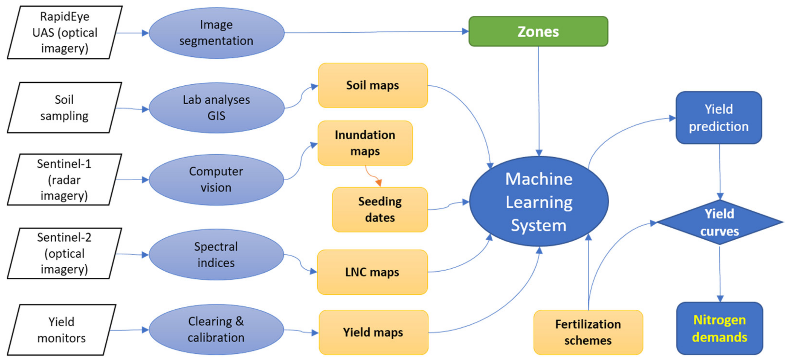
Finally, the measured soil properties, the rice growth (in terms of days after seeding), the LNC values before fertilization, and yield records per zone were inserted into Machine Learning Systems (MLS) to train yield prediction algorithms. Using the trained algorithms, alternative fertilization schemes were tested, with the optimum one selected according to the resulting yield curves (

Table 2. A summary of the methodological steps accomplished, and technologies used.

Steps	Technologies	Years
1. Zone delineation	Segmentation of RapidEye (a) and ancillary visual interpretation of Unmanned Aerial System (UAS) data (b)	2015 (a) 2016 (b)
2. Soil sampling	Global Positioning System (GPS)-guided field surveys	2016–2018
3. Inundation mapping	Convolution neural network (CNN), Computer Vision, with Sentinel-1 (SAR data)	2017–2019
4. Growth stage determination	Time-series analysis	2017–2019
5. Leaf nitrogen concentration (LNC) mapping	Spectral indices derived from Sentinel-2 (optical data)	2016–2019
6. Zonal applications	Manually (2016)	2016–2019
	Variable-Rate Technologies (VRT) (2017–2019)
7. Yield mapping	Yield mapper mounted on harvester	2017–2019
8. Yield prediction	Machine learning	2017–2019
9. N-demand suggestions	Optimal Nitrogen-yield curves	2017–2019

). A workflow between the different parts of the methodology is illustrated in Figure 2.

4. Data Ingestion

A multi-source, multi-temporal, and multi-scale dataset, comprising Earth observation imagery, soil data, yield maps, and historic records, was collected for the needs of the current research (

Table 3. A summary of the dataset used.

Data Type	Description	Multitude/Format	Years
Earth Observation	RapidEye imagery	3 image scenes	2015
	UAS imagery	1 image scene	2016
	Sentinel-1 imagery	14 image scenes	2018–2019
	Sentinel-2 imagery	4 image scenes	2016–2019
Soil samples	Eighteen soil properties	146 locations	2016–2018
Yield maps	Continuous yield surfaces	3 raster layers	2017–2019
Historic data	Tabular records	18 Excel files	1998–2019

). Specifically, RapidEye satellite scenes were acquired on three different dates during the cultivation season of 2015, while ancillary UAS image was acquired exactly before the beginning of the first cultivation season (April 2016). Fourteen Sentinel-1 and four Sentinel-2 image scenes were acquired throughout the period 2016–2019.

In parallel, a set of soil samples at 146 locations was collected from all over the rice farm and in different years (2016–2018, in wintertime); on average, 1 sample corresponded to an area of 0.76 ha, or 1.3 samples were collected per hectare. Yield maps were recorded by a harvester equipped with a yield monitoring system for three consecutive years (2017–2019). Finally, historic data were provided in tables since 1998, including detailed calendars on all the farming practices followed and annual yield figures per field.

Given that datasets are never perfect, however, data preparation for predictive modelling purposes means to bring the dataset as closely as possible to model specifications or to adapt a model to the properties of the dataset [20]. In the following paragraphs, preparation of the collected data and their conversion into input parameters to the tested models is presented.

4.1. Zone Delineation and Soil Sampling

A methodology appropriate for detecting local variation in image data and thus delineating management zones (for precision farming applications) is image segmentation. Segmentation is defined as the procedure of image division into spatially continuous, disjointed, and homogeneous regions, called image objects [21]. The Fractal Net Evolution Approach (FNEA) segmentation algorithm (also known as “Multiresolution Segmentation”) was applied with a time series of three RapidEye images acquired on 30 May 2015, 4 July 2015, and 26 August 2015. A composite consisting of 15 image bands (5 bands per image × dates) was prepared for the analysis.

RapidEye was the first commercial optical imagery to supply an individual band in the red edge wavelengths, which is linked to critical crop parameters, such as chlorophyll content, biomass, and water content [22]. The RapidEye image dataset used in this research was a radiometrically corrected and orthorectified product (3A-level), in the WGS84 projection, UTM zone 34. The pixel size of the images was 5 m.

With FNEA, image objects are created by grouping single pixels through a stepwise region-growing procedure of minimizing internal heterogeneity within each object until a pre-defined threshold (called “scale factor”) is reached. Scale factor influences the desired object size and shape, according to one spectral and two shape criteria; namely, cumulative standard deviation of each of the input spectral bands and compactness and smoothness, respectively [23].

The object-based analysis targeted at a mean object size which would correspond to management zones of about 1.5 ha, thus covering the requirement for a density of 1 sample per 2 ha, suggested for cereals by Wetterlind et al., (2008) [24]. With a trial-and-error segmentation approach, it was found that a scale factor of 150 resulted in the desired output. After clearing the very small or long-shaped zones (in practice, by merging them with their closest neighboring zone-polygon), 62 zones were delineated. Four extra zones were detected with visual photointerpretation of multispectral images (Visible-NIR) taken by an unmanned aerial system (UAS) close before the beginning of the 2016 cultivation season (i.e., in bare soil). Thus, the final number of zones was 66. According to Karydas et al., (2020) [25], the specific zonation achieved to reduce soil variation by 18.6% compared to the conventional uniform applications, while it increased precision in fertilization applications by 24.5%.

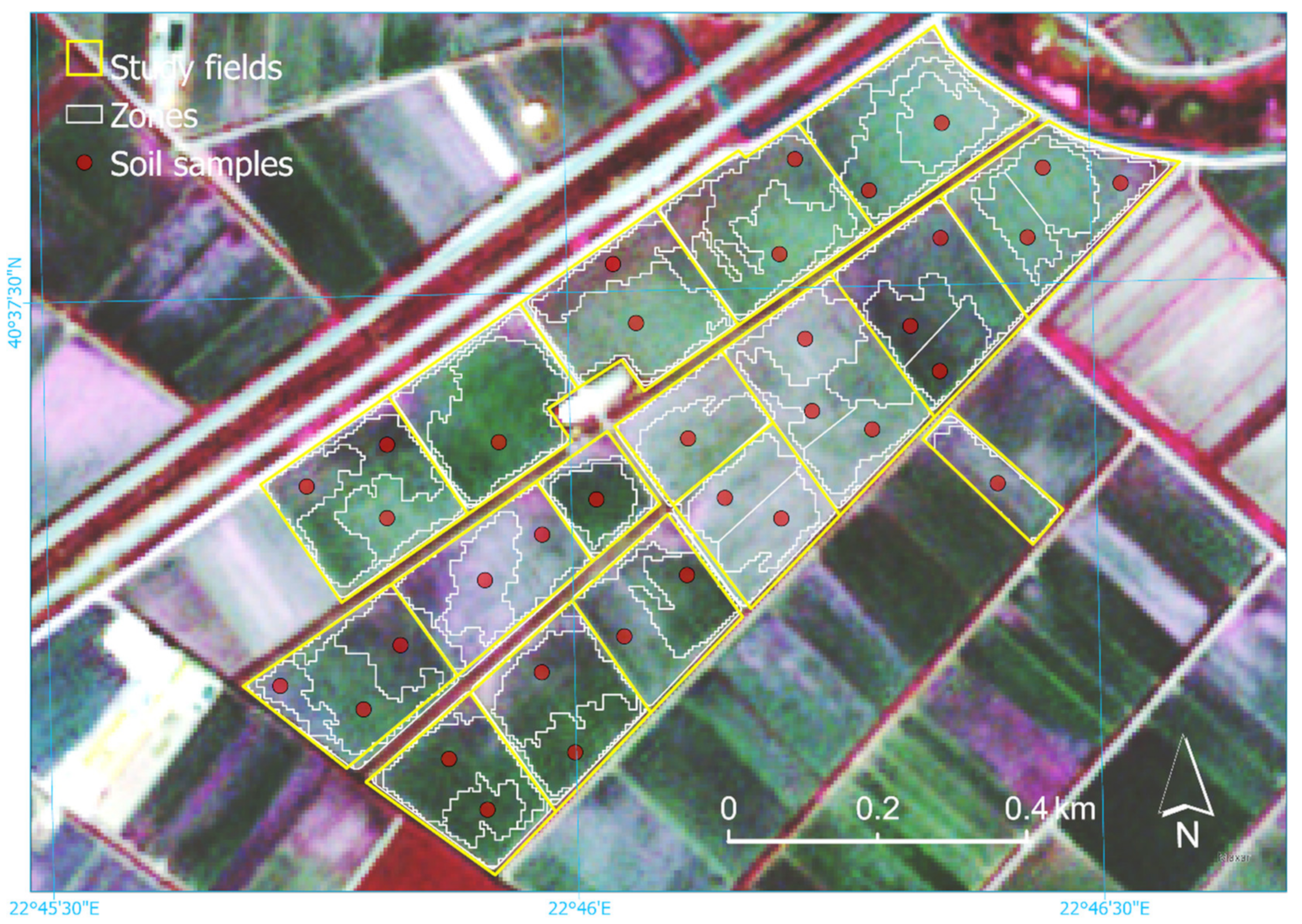
An equal number of soil samples were collected from the centroids of each management zone (Figure 3). The samples were extracted from 3 locations (sub-samples) around every centroid, distancing by about 5 m, at a 30 cm depth, and underwent full analyses (for 18 physical and chemical properties) in the State Laboratory of Soil and Water Resources Institute in Thessaloniki.

Using the Moran’s I test for assessing spatial autocorrelation at the sampled locations with the 2016 soil data, it was shown that all physical and chemical soil properties were highly clustered, with z-score values ranging from 2.67 to 42.7. This implies that the density of the initial soil sampling scheme provided enough critical information on the spatial distribution of the soil properties in the specific farm, thus verifying the assumption of representativeness of the samples throughout the study farm [15].

4.2. Inundation Mapping and Seeding Date Determination

The seeding date was determined through the detection of fields’ inundation, as seeding follows shortly after rice fields’ inundation. The inundations were mapped with Computer Vision techniques applied on Synthetic Aperture Radar (SAR) images acquired from Sentinel-1 satellites (for the years 2018–2019) [26,27]. However, the growers in some cases, according to the levels of infestation by the red rice (Oryza punctate), use a weed suppressive period following an early inundation of the field. Hence, critical for the scopes of the MLS approach used in this study was to identify this period, which can be called “pseudo-seeding”. Therefore, if the first inundation was followed by a short fallow period, the seeding date was considered the date of the second inundation.

Inundation mapping was carried out by classifying land into 2 exclusive classes (WATER vs. NO-WATER). Sentinel-1 products were chosen for inundation mapping because they offer medium-to-high-resolution imaging in all weather conditions, due to the C-SAR sensor mounted on the satellites. Sentinel-1 images are acquired every 6 days by a two-satellite constellation, with the prime objectives of Land and Ocean monitoring.

A total of 14 Sentinel-1 image scenes covering the study fields in the Plain of Thessaloniki from the 2018 and 2019 rice cropping seasons were acquired; the exact dates were: 18 May 2018, 5 June 2018, 23 June 2018, 23 July 2018, 10 August 2018, 22 August 2018, 15 September 2018, 25 May 2019, 31 May 2019, 12 June 2019, 18 July 2019, 5 August 2019, 29 August 2019, and 22 September 2019. The first acquisition dates correspond to several weeks before the normal commencement of the rice period in Thessaloniki; N topdressing normally takes place at the end of June for rice seeded in May.

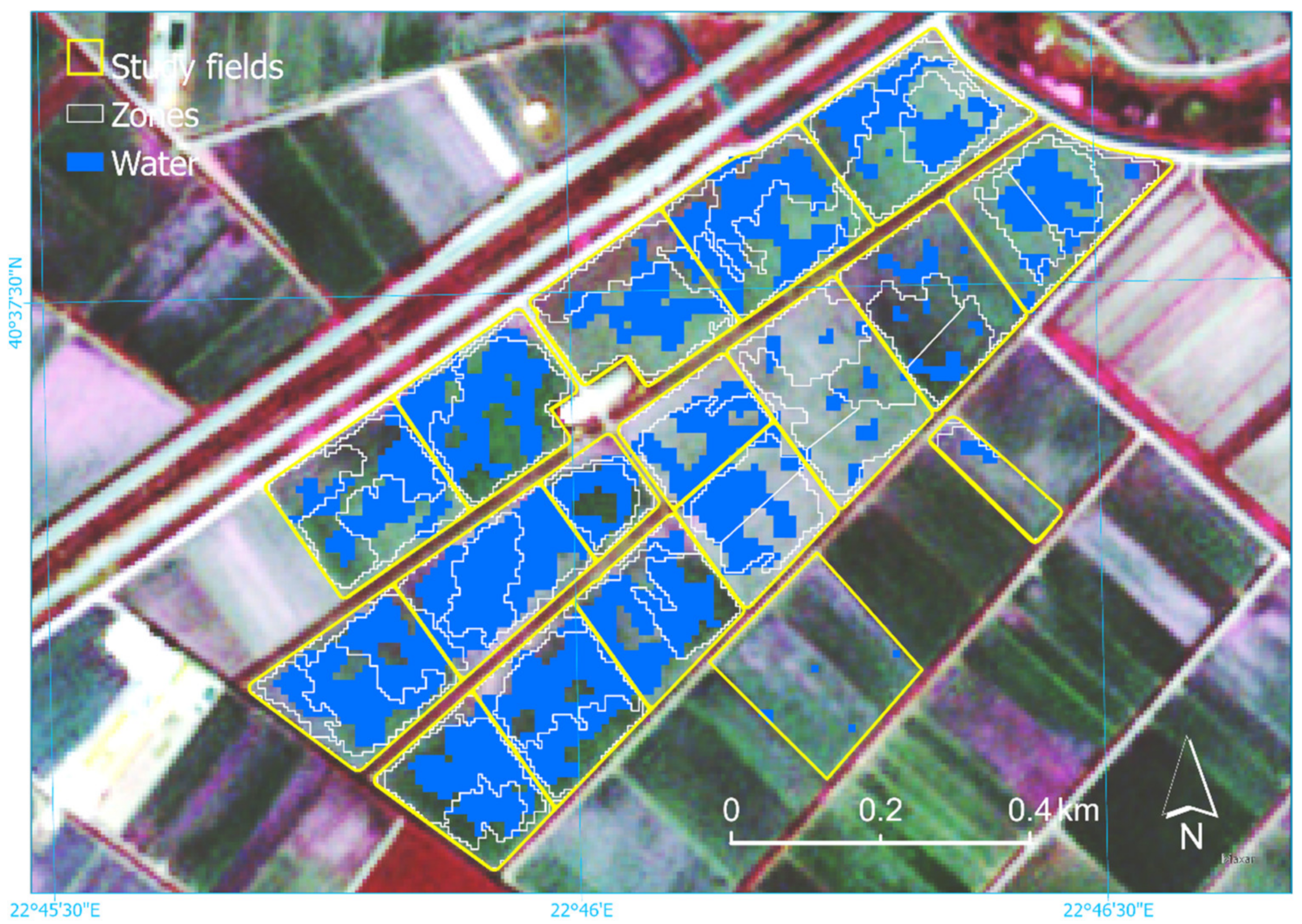
First, SNAP-ESA software was used to edit the Sentinel-1 imagery for calibration, speckle filtering, and terrain correction. Then, QGIS software was used to create the “Areas of Interest” (AOIs) according to the training field data. Finally, the edited images were masked with the AOIs, thus creating the required clipped image subsets for the analysis (Figure 4). To facilitate the whole process of image subset preparation, a script was written in Python programming language.

The image data were analyzed with Computer Vision using a Convolutional Neural Network (CNN). According to Jan Eric Solem (2012) [28], Computer Vision is the automated extraction of information from images. The Computer Vision problems most commonly use Convolutional Neural Networks (CNNs), a class of Deep Neural Networks that are widely used in image recognition and image classification because they are capable of discovering the relevance in contextual features [29].

The architecture of network construction was to include three 2D convolution layers that were activated with the ReLU function. A dense layer activated with the ReLU function was used to connect all the neurons which ended up in the final neuron that conducted the categorization. This final neuron is activated with the sigmoid function. The CNN was trained in 7 epochs and with 10 steps per epoch, as after many trials these attributes yielded the best result without overfitting the data in the model.

Samples for training and validation of the CNN were collected with field surveys on the same dates of the Sentinel-1 images and consisted of 280 image subsets (polygons) covering wetlands and rice fields. Part of these subsets (210 samples) were used for training the model, while the rest (70 samples) were used for validation. From the training samples, half corresponded to WATER class and half corresponded to NO-WATER class.

The model achieved a precision of 0.92, a recall of 0.93 and a F1-score of 0.92 for the WATER class. For CNN training and verification, the Keras ImageDataGenerator library was employed, while the images were rescaled in 1/255 and resized to 120 × 120 px.

4.3. LNC Mapping, Applications, and Yield Mapping

Leaf nitrogen concentration (LNC) is an important index of photosynthetic capacity of crops [30]. LNC is necessary to farmers for making their decisions on fertilization, especially the topdressing ones [31]. Remote sensing has been widely used in LNC estimations in crops on a large geographic scale [7,8,9], as rapid determination of LNC could provide valuable information for monitoring crop physiology to the farmers [5]. In this direction, precision agriculture applications can improve use efficiency of nitrogen fertilizers [6]. The common practice is to establish linear or nonlinear relationships between leaf N content and spectral features derived from leaf reflectance spectra.

In this research, LNC was estimated from Sentinel-2 images acquired on a variety of dates over the 4-year study period: 06 July 2016, 21 July 2016, 16 August 2016, 18 June 2017, 28 June 2017, 28 July 2017, 27 August 2017, 8 June 2018, 13 July 2018, 18 July 2018, 28 July 2018, 22 August 2018, 13 June 2019, 28 June 2019, 18 July 2019, 28 July 2019, and 1 September 2019. However, only a part of the LNC maps were used by the grower to support his decisions on N-fertilization; those acquired close before the planned topdressing applications (i.e., 06 July 2016, 28 June 2017, 13 July 2018, and 28 June 2019).

Sentinel-2 is free and ready-to-use, high-resolution optical imagery by the European Space Agency (ESA). Its MultiSpectral Instrument (MSI) carries 13 spectral bands ranging from the visible and near infrared to the short-wave infrared. The spatial resolution varies from 10 to 60 m, depending on the spectral band, with a 290 km field of view. This unique combination of high spatial resolution, wide field of view and broad spectral coverage, together with free availability of ready-to-use products in an atmospherically corrected reflectance mode, has opened a new window in operational land use mapping [32].

Leaf Nitrogen Concentration (LNC) was estimated and mapped using equations established originally from hyperspectral data by Stroppiana et al., (2011) [33], here applied with Sentinel-2 imagery as follows:

$$LNC=4.060·NDRE+0.43$$

(1)

where $NDRE$: the Normalized Difference RedEdge index;

$$NDRE=\left(R790-R720\right)/\left(R790+R720\right)$$

(2)

where $R720:$ reflectance at 720 nm or Band-5 for Sentinel-2; $R790:$ reflectance at 790 nm or Band-9 for Sentinel-2. Using an available multi-temporal hyperspectral dataset from experimental rice plots, the LNC values were calibrated according to the exact wavelengths of Equation (2) vs. Sentinel-2 band wavelengths and for the exact seeding date of each field; relevant work on the specific hyperspectral dataset can be found in Karydas (2016) [34].

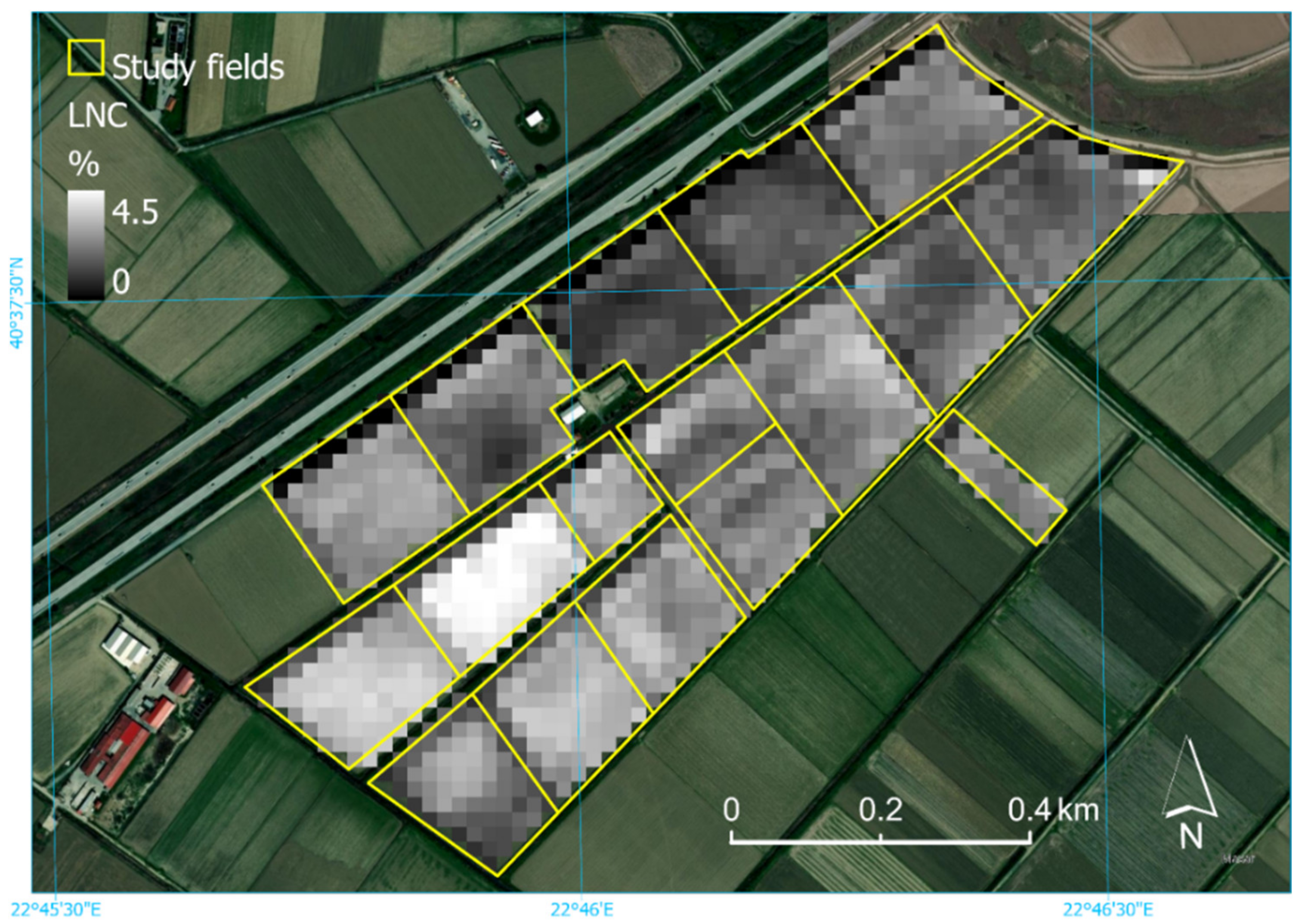
The Leaf Nitrogen Content (LNC) was estimated using the latest cloud-free Sentinel-2 images available before the nitrogen topdressing applications (Figure 5). Based on the mapping outputs, a concrete N-dose was recommended to the grower per management zone.

The fertilizers were applied with a Variable Rate Technology (VRT) system, namely, a Kverneland Geospread model with a Tellus Pro terminal. The GEOSPREAD system on the Kverneland disc spreaders enables farmers to reduce the spreading pattern in sections of 1 m with the highest accuracy.

The Tellus PRO terminal is the center for connecting all ISOBUS machines and a platform for running precision farming applications. The terminal was supplied with the digital maps containing the fertilization recommendations (one polygon per management zone) in the appropriate format (i.e., after their conversion from shapefiles to XML files).

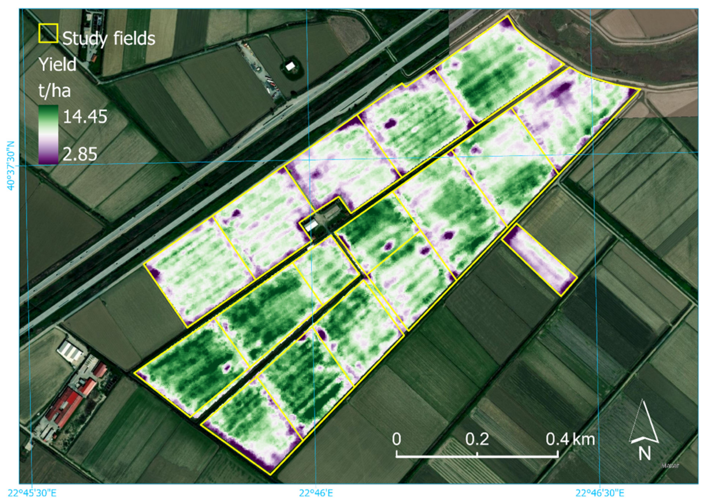
Yield values per zone were derived from annual yield maps (except cultivation year 2016). Rice yield was mapped with a 7.5 m wide Trimble yield monitor mounted on a Claas harvester; guidance and field scanning were automated. The original data were cleared from unrealistic values and calibrated with weighted rice yield data per field (provided by the grower) (Figure 6).

5. Modelling

5.1. Background

Four machine learning algorithms were tested towards yield prediction from the available dataset: Extreme Gradient Boosting (XGBoost), Random Forest (RF), Support Vector Regression (SVR) and Elastic Net (ElasticNet).

The XGBoost is a decision tree-based algorithm, which gives state-of-the-art results in many machine learning problems, as it uses the gradient boosting framework and also focuses on areas within the dataset of high error for improving the overall initial predictor [11]. This technique is dynamic as it leaves out the data that fit in the weak models and focuses on the development of new models that can better deal with the remaining data [35]. XGBoost can model difficult problems with multiple variables. Ultimately, the aim of XGBoost is to convert a low statistical hypothesis to a stronger statistical hypothesis, providing a predictive model with high prediction accuracy by combining moderately inaccurate models [36]. However, the efficiency of XGBoost relies much on the optimal selection of the hyperparameters. XGBoost is relatively sensitive to overfitting and maximization of variance, as it tries to focus on areas with high error within the dataset. A key technique that must be included in the model for addressing this problem is the dropout technique and more specifically the adjustment of the early stopping rounds parameter.

Random Forest is also a dynamic technique as it is an improvement of bagged decision trees. The decision trees are constructed by sampling the original training set with replacement in a way that reduces the correlation between the individual trees. This is done by choosing a random sampling of training data when building trees and a random subset of features in each split. Finally, the predictions are made by averaging the predictions of each decision tree [37]. This method aids in dealing with the overfitting problem encountered by simple decision trees algorithms, and finally this technique leads to the minimization of bias, but it is also sensitive to high variance.

Support Vector Regression (SVR) is a dynamic technique that creates a hyperplane separating the data classes by maximizing the margin between the classes’ closest points [38]. There are also two other lines, called boundary lines, which create a margin. This boundary margin separates the data classes in SVR and tries to fit the error within this boundary margin. Finally, the SVR finds the hyperplane that has the maximum observation points within the boundary lines [39].

ElasticNet is suggested by Zou and Hastie 2005 [40] as useful when the number of variables is high, the number of observations is small, and when there are variables strongly correlated to each other. This type of regression is between Ridge Regression and Lasso Regression. If there is a subset of the total number of features that are useful for the prediction, then it is preferable to use Lasso Regression over Ridge Regression. However, as there is a regularization parameter which controls if the Elastic Net Regression works more like a Ridge Regression or Lasso Regression, it is preferred to use Elastic Net Regression over Lasso and Ridge Regression. The strength of the Elastic Net algorithm is that it can work as a mix of these types of regression. Moreover, Elastic Net is still preferred over Lasso if there is collinearity between the features and it also overcomes the problem of overfitting in which the simple linear regression is highly susceptible.

5.2. Model Configurations

The implemented models took input from the measured soil properties, the cultural practices (variety and broadcasting units), the growth stage, the LNC, and the yield. Growth stage and cultural practices can affect modelling stability in operational remote sensing solutions, and thus it was found necessary to be included in model building [41]. However, other equally important parameters, such as weather conditions, water regime, soil microbial activity, soil compaction, sun irradiance, etc. [42], were not available.

Eighteen soil properties were available from the laboratorial analyses in numerical format. Two varieties were cultivated in the pilot farm during the study period: Ronaldo and Bonnet; the former variety was denoted as VARIETY_1 and the latter as VARIETY_2 in the input list of features. The growth stage was denoted as DATE and was recorded as number of days after seeding. Six growth stages can be recognized in rice [2]: early vegetative stage following sowing, mid-to-late vegetative stage (mid-tillering), early reproductive stage (panicle initiation to booting), mid-to-late reproductive stage (heading to flowering), ripening stage and harvest stage. Normally, the N topdressing application in Greece occurs at the early reproductive stage and more specifically around the booting stage. The LNC was recorded numerically and the yield as well.

In addition to the single parameters, though, a combination of LNC with growth stage (in terms of a multiplication: LNC*DATE) was also tested. The reason is that LNC alone does not consider the relativity of rice growth, which was represented by the introduced combination.

Prior to model running, the dataset was checked using multicollinearity diagnostics with the Mctest package in R [43], in order to detect collinearity in the dataset among regressors on the yield variable. All the variables which remained after multicollinearity were scaled and power transformed using the StandardScaler of the Scikit-Learn library for feeding the algorithms [44].

The dataset was randomly separated into training and test parts consisting of 70% (183 samples) and 30% (91 samples) of the total data, respectively. The algorithms were trained either including the growth stage (denoted as DATE) or without, by selecting optimal parameters in every case. The XGBoost and Random Forest models were configured both for runs with the inclusion of the DATE and LNC*DATE parameters and without them. The algorithms were written in Python programming language [45]; the optimized hyperparameters for all models are presented in

Table 4. A summary of the dataset used in the current research.

Hyperparameter	XGBoost	RF	SVR	ElasticNet
learning_rate	0.03	-	-	-
max_depth	5 (3) *	90 (80)	-	-
n_estimators	100	1000 (100)	-	-
subsample	0.8 (0.5)	-	-	-
early_stopping_rounds	42	-	-	-
min_samples_leaf	-	2 (4)	-	-
min_samples_split	-	2 (5)	-	-
C	-	-	100	-
gamma	-	-	0.01	-
epsilon	-	-	0.1	-
kernel	-	-	rbf	-
alpha	-	-	-	0.1
l1_ratio	-	-	-	0.0
max_iter	-	-	-	5

* in brackets, hyperparameter values for model runs without the DATE and LNC*DATE variables.

.

5.3. Yield Curves

One of the safest ways to estimate economically vital fertilization applications is to create graphs of yield vs. fertilization units. According to this technique, the optimum fertilization dose is determined where yield begins to decrease [46,47]. In this research, yield-nitrogen curves were created for different standard fertilization schemes the grower follows over the years, and specifically, for doses starting from 210 up to 260 kg ha⁻¹.

When the optimum total nitrogen demand (or applied dose, Nneed) is specified from the yield curves, the topdressing nitrogen demands (Ntopdressing) per zone can be determined, by subtracting the broadcasting nitrogen demand (Nbroadcasting), which is usually equal to a constant value (160 kg ha⁻¹ for the study area), from the former.

6. Results and Discussion

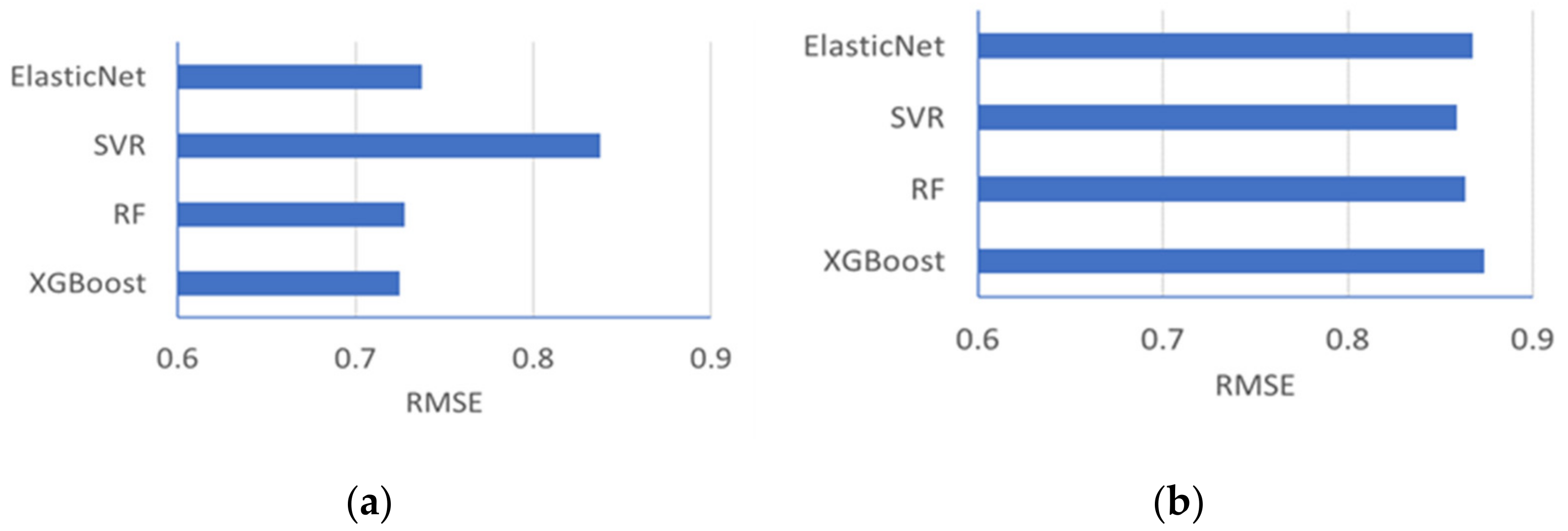
Using the Root Mean Square (RMS) error between the predicted and observed yield values (from the yield maps) in the relevant years (2017–2019) for all the tested models, it was found that the XGBoost model resulted in the lowest error compared to the other three models (0.73 tn ha⁻¹) provided, though, that DATE and LNC*DATE parameters were not included in the algorithm; otherwise, RMS error was found quite high in all cases. In practice, only SVR gave high RMS error in both cases, thus any of the three models, i.e., XGBoost, RF, and ElasticNet, could be selected for the analysis.

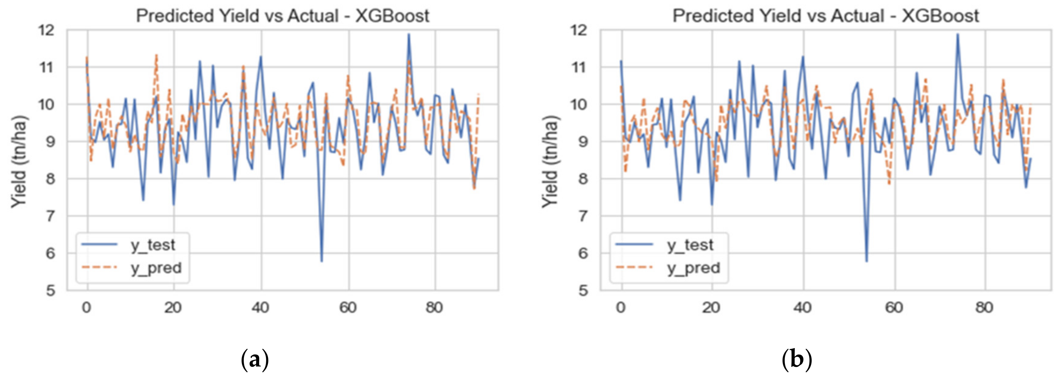
Finally, the XGBoost model was selected for two reasons: (a) it was found more appropriate for the specific dataset, and (b) it performed slightly better than the other three models in the case of DATE inclusion (Figure 7). Furthermore, XGBoost performed better when the DATE was included in the parameters, as the difference between the observed and predicted values was reduced (Figure 8).

Among the included parameters, VARIETY_1 (medium-size grain rice variety) was the most influencing parameter for the XGBoost either with or without inclusion of DATE parameter (Figure 9). For the optimally parameterized model, the DATE and LNC*DATE variables are highly weighted.

Although soil properties showed to have lower values of relative importance compared to VARIETY, DATE, and LNC*DATE, their importance cannot be ignored, particularly for pH, calcium carbonate (CaCO3), potassium (K), organic matter (OM), and phosphorus (P). Nitrogen (N) is the most deficient nutrient for rice growing in Greece, and this is the reason it is provided in larger amounts compared to other nutrients. However, the N supplied to the rice crop was not considered as a significant feature in the models. Possibly, this has to do with the fact that the grower tends to oversupply with N. Thus, normally in many cases, N supply exceeds crop demand. This is the scope though of the MLS constructed in this research, i.e., to identify the delineated zones where excessive N would limit yield.

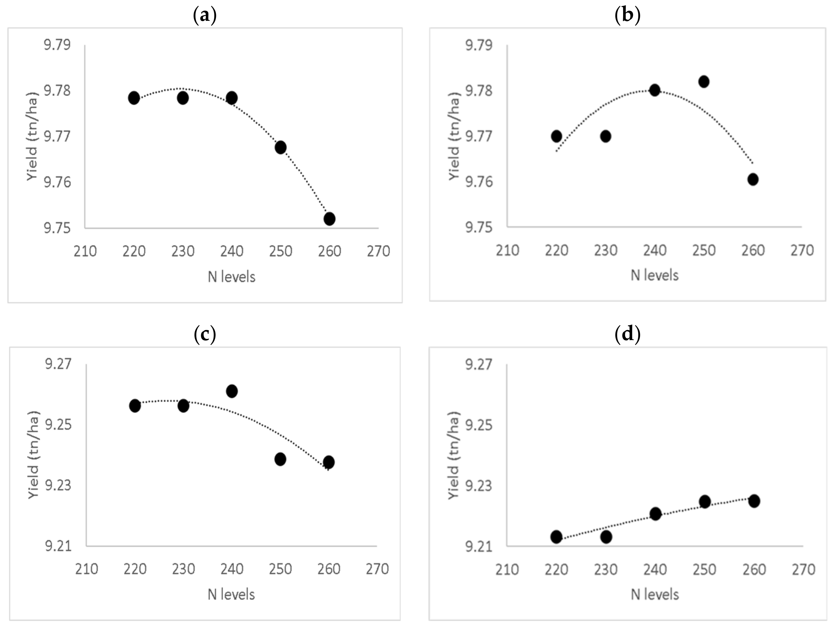
The yield curves indicated that there is clear yield reduction when rice is supplied with more than 240 to 250 kg of nitrogen per hectare in all management zones. In other words, there is no yield benefit when rice is supplied with more than 250 kg of nitrogen per hectare in all cases (Figure 10).

The presented curves in Figure 10 show that the yield range between the zones is small (9.21–9.78 t/ha) for the different N levels. This occurs because the N_need parameter representing the N fertilization rate, as shown in Figure 9, scores low in the feature importance plot. This is obviously because it is a general practice for rice growers to oversupply with N. Thus, the extra N nutrition (higher than 240 kg N per ha) usually does not provide any yield benefit. Therefore, the scope of the developed algorithm, which was presented in the current work, was to detect cases of field zones where the extra N nutrition will not provide any yield benefit. The advantage of this methodology is the reduction of inputs for the rice growers and obviously environmental benefits can be realized by the adoption of this algorithm. In Figure 8 though, there are observations that they are markedly different in terms of yield, including zones characterized by low yields such as 6 tn per ha. These outliers frequently occur in commercial practice and have to do with completely different aspects than the fertilization parameter and have more to do with failure of herbicide applications or disease outbreaks (such as Pyricularia oryzae).

Apart from defining optimal N-doses, management zone delineation has given insight about the P and K deficiencies, and all the other physical and chemical properties explaining yield variance. P deficiency of rice in Greece is quite common, as Greek soils are highly calcic, while K have been supplied for several years in Thessaloniki Plain in low amounts, causing serious K deficiency in some of the zones. The growers tend to use low amounts of K fertilizer to reduce the fertilizer cost, and there is a general perception that K deficiency is uncommon for rice growing in Thessaloniki. Covering P and K demand allowed the model to better explain the effect of LNC (as an index correlated with N uptake), on yield variance.

The rice growers in the Plain of Thessaloniki tend to use an NPK 32-5-5 fertilizer (containing mostly nitrogen and providing low concentrations of phosphorus and potassium), due to high potassium supplying capacity of many soils and the increased phosphorus availability under flooded conditions. However, phosphorus and potassium availability depend on soil texture [3] and the continuous use of the same fertilizer management approach has resulted in unbalanced fertility within the field parcels. If an efficient nitrogen topdressing management advice is provided to the growers timely, the spatial availability of P and K can also be addressed; P and K explain a large proportion of the yield variance [3]. Fertility issues of rice cultivation in the soils of the area have been discussed by [18].

7. Conclusions

Using machine learning systems, this 4-year study in a pilot rice farm of about 110 hectares in Greece resulted in a predictive model for topdressing nitrogen demands solely from soil and satellite data. The required dataset was derived mainly from open-source satellite data (Sentinel-1 and Sentinel-2 imagery), limited field surveys (for soil sampling), and records from the farmer’s machinery (yield maps); Sentinel-2 scenes could also be used for management zone delineation instead of RapidEye images if the latter were not available; the use of UAS imagery was only ancillary and could be skipped, too.

Model building helped in better understanding fertility issues in the soils of the area, and finally, in providing thorough and timely suggestions to the grower. In parallel with its main goal, the study also achieved to produce an algorithm for mapping inundated rice fields and thus indicate seeding dates, which proved to be a critical variable in the prediction process. It is foreseen that by entering additional variables to the model, such as weather conditions, water regime within the field, weed infestations, and diseases, would further improve model performance.

The developed model (an XGBoost model) can be considered as fully operational, repeatable, and possibly expandable to larger rice cultivation areas. Used as a paradigm, the model would allow reduction of fertilizer costs for growers and could have a significant positive effect in the protection of waters.

With a steadily view to supporting growers’ decision making, Ecodevelopment S.A. is planning to expand the application of the new predictive model in different study areas, thus empowering the generality of the proposed approach.

References

- Hou, W.; Tränkner, M.; Lu, J.; Yan, J.; Huang, S.; Ren, T.; Cong, R.; Li, X. Diagnosis of Nitrogen Nutrition in Rice Leaves Influenced by Potassium Levels. Front. Plant Sci. 2020, 11, 165. [Google Scholar] [CrossRef]
- Williams, J.F. Rice Nutrient Management in California; UCANR Publications: Davis, CA, USA, 2010. [Google Scholar]
- Iatrou, M.; Karydas, C.; Iatrou, G.; Zartaloudis, Z.; Kravvas, K.; Mourelatos, S. Optimization of fertilization recommendation in Greek rice fields using precision agriculture. Agric. Econ. Rev. 2018, 19, 64–75. [Google Scholar]
- Ranatunga, T.; Hiramatsu, K.; Onishi, T.; Ishiguro, Y. Process of denitrification in flooded rice soils. Rev. Agric. Sci. 2018, 6, 21–33. [Google Scholar] [CrossRef]
- Robertson, G.; Groffman, P. Nitrogen Transformations. In Soil Microbiology Ecology Biochemistry, 4th ed.; Academic Press: Burlington, MA, USA, 2015; pp. 421–446. [Google Scholar] [CrossRef]
- Huang, S.; Zhao, C.; Zhang, Y.; Wang, C. Nitrogen Use Efficiency in Rice. In Nitrogen in Agriculture—Updates; Intechopen: London, UK, 2018. [Google Scholar] [CrossRef]
- Yousaf, M.; Li, J.; Lu, J.; Ren, T.; Cong, R.; Fahad, S.; Li, X. Effects of fertilization on crop production and nutrient-supplying capacity under rice-oilseed rape rotation system. Sci. Rep. 2017, 7, 1–9. [Google Scholar] [CrossRef]
- Tang, L.; Zhu, Y.; Hannaway, D.; Meng, Y.; Liu, L.; Chen, L.; Cao, W. RiceGrow: A rice growth and productivity model. NJAS Wagening. J. Life Sci. 2009, 57, 83–92. [Google Scholar] [CrossRef]
- Bouman, B.A.M.; Kropff, M.; Tuong, T.; Wopereis, M.; ten Berge, H.; van Laar, H. ORYZA2000: Modeling Lowland Rice; IRRI: Los Baños, Philippines, 2001; 235p. [Google Scholar]
- Gómez, D.; Salvador, P.; Sanz, J.; Casanova, J.L. Potato Yield Prediction Using Machine Learning Techniques and Sentinel 2 Data. Remote Sens. 2019, 11, 1745. [Google Scholar] [CrossRef]
- Karydas, C.; Iatrou, M.; Kouretas, D.; Patouna, A.; Iatrou, G.; Lazos, N.; Gewehr, S.; Tseni, X.; Tekos, F.; Zartaloudis, Z.; et al. Prediction of Antioxidant Activity of Cherry Fruits from UAS Multispectral Imagery Using Machine Learning. Antioxidants 2020, 9, 156. [Google Scholar] [CrossRef]
- Chlingaryan, A.; Sukkarieh, S.; Whelan, B. Machine Learning Approaches for Crop Yield Prediction and Nitrogen Status Estimation in Precision Agriculture: A Review. Comput. Electron. Agric. 2018, 151, 61–69. [Google Scholar] [CrossRef]
- Whelan, B.; Taylor, J. Precision Agriculture for Grain Production Systems. Field Crops Res. 2013, 155, 133. [Google Scholar]
- Pantazi, X.E.; Moshou, D.; Mouazen, A.M.; Alexandridis, T.; Kuang, B. Data fusion of proximal soil sensing and remote crop sensing for the delineation of management zones in arable crop precision farming. CEUR Workshop Proc. 2015, 1498, 765–776. [Google Scholar]
- Peng, S.; Buresh, R.J.; Huang, J.; Zhong, X.; Zou, Y.; Yang, J.; Wang, G.; Liu, Y.; Hu, R.; Tang, Q.; et al. Improving nitrogen fertilization in rice by sitespecific N management. A review. Agron. Sustain. Dev. 2010, 30, 649–656. [Google Scholar] [CrossRef]
- Pantazi, X.; Moshou, D.; Alexandridis, T.; Whetton, R.; Mouazen, A. Wheat yield prediction using machine learning and advanced sensing techniques. Comput. Electron. Agric. 2016, 121, 57–65. [Google Scholar] [CrossRef]
- Liakos, K.G.; Busato, P.; Moshou, D.; Pearson, S.; Bochtis, D. Machine learning in agriculture: A review. Sensors 2018, 18, 2674. [Google Scholar] [CrossRef] [PubMed]
- Aschonitis, V.; Karydas, C.G.; Iatrou, M.; Mourelatos, S.; Metaxa, I.; Tziachris, P.; Iatrou, G. An Integrated Approach to Assessing the Soil Quality and Nutritional Status of Large and Long-Term Cultivated Rice Agro-Ecosystems. Agriculture 2019, 9, 80. [Google Scholar] [CrossRef]
- PrecisionAG. ISPA Forms Official Definition of ‘Precision Agriculture’. 2019. Available online: https://www.precisionag.com/market-watch/ispa-forms-official-definition-of-precision-agriculture/ (accessed on 26 March 2021).
- Karydas, C.G.; Panagos, P.; Gitas, I.Z. A classification of water erosion models according to their geospatial characteristics. Int. J. Digit. Earth 2012, 7, 229–250. [Google Scholar] [CrossRef]
- Blaschke, T. Object based image analysis for remote sensing. ISPRS J. Photogramm. Remote Sens. 2010, 65, 2–16. [Google Scholar] [CrossRef]
- Filella, I.; Penuelas, J. The red edge position and shape as indicators of plant chlorophyll content, biomass and hydric status. Int. J. Remote Sens. 1994, 15, 1459–1470. [Google Scholar] [CrossRef]
- Kim, M.; Madden, M.; Warner, T. Estimation of Optimal Image Object Size for the Segmentation of Forest Stands with Multispectral IKONOS Imagery. In Object-Based Image Analysis: Spatial Concepts for Knowledge-Driven Remote Sensing Applications; Blaschke, T., Lang, S., Hay, G.J., Eds.; Springer: Berlin/Heidelberg, Germany, 2008; pp. 291–307. [Google Scholar] [CrossRef]
- Wetterlind, J.; Stenberg, B.; Söderström, M. The use of near infrared (NIR) spectroscopy to improve soil mapping at the farm scale. Precis. Agric. 2008, 9, 57–69. [Google Scholar] [CrossRef]
- Karydas, C.; Iatrou, M.; Iatrou, G.; Mourelatos, S. Management Zone Delineation for Site-Specific Fertilization in Rice Crop Using Multi-Temporal RapidEye Imagery. Remote Sens. 2020, 12, 2604. [Google Scholar] [CrossRef]
- Čotar, K.; Oštir, K.; Kokalj, Ž. Radar Satellite Imagery and Automatic Detection of Water Bodies. Geode Glass 2016, 50, 5–15. [Google Scholar]
- Nemni, E.; Bullock, J.; Belabbes, S.; Bromley, L. Fully Convolutional Neural Network for Rapid Flood Segmentation in Synthetic Aperture Radar Imagery. Remote Sens. 2020, 12, 2532. [Google Scholar] [CrossRef]
- Solem, J.E. Programming Computer Vision with Python; O’Reilly Media: Newton, MA, USA, 2012. [Google Scholar]
- Maggiori, E.; Tarabalka, Y.; Charpiat, G.; Alliez, P. Convolutional Neural Networks for Large-Scale Remote-Sensing Image Classification. IEEE Trans. Geosci. Remote Sens. 2017, 55, 645–657. [Google Scholar] [CrossRef]
- Evans, J.R. Photosynthesis and nitrogen relationships in leaves of C3 plants. Oecologia 1989, 78, 9–19. [Google Scholar] [CrossRef]
- Ladha, J.K.; Pathak, H.; JKrupnik, T.; Six, J.; van Kessel, C. Efficiency of Fertilizer Nitrogen in Cereal Production: Retrospects and Prospects. Adv. Agron. 2005, 87, 85–156. [Google Scholar]
- Torma, M.; Hatunen, S.; Harma, P.; Jarvenpaa, E. Sentinel-2 Images and Finnish Corine Land Cover Classification. In First Sentinel-2 Preparatory Symposium [Internet]; Finnish Environment Institute: Helsinki, Finland, 2012; p. 20. [Google Scholar]
- Stroppiana, D.; Fava, F.; Boschetti, M.; Brivio, P. Estimation of Nitrogen Content in Crops and Pastures Using Hyperspectral Vegetation Indices. In Hyperspectral Remote Sensing of Vegetation; CRC Press: Boca Raton, FL, USA, 2011; pp. 245–262. [Google Scholar]
- Karydas, C.G. Temporal dimensions in rice crop spectral profiles. J. Geomat. 2016, 10, 140–148. [Google Scholar]
- Chen, T.; Guestrin, C. XGBoost: A Scalable Tree Boosting System. In Proceedings of the 22nd ACM SIGKDD International Conference on Knowledge Discovery and Data Mining, San Francisco, CA, USA, 13–17 August 2016. [Google Scholar] [CrossRef]
- Brownlee, J. XGBoost with Python, Gradient Boosted Trees with XGBoost and Scikit-Learn; Machine Learning Mastery: San Juan, PR, USA, 2018. [Google Scholar]
- Breiman, L. Random forests. Mach. Learn. 2001, 45, 5–32. [Google Scholar] [CrossRef]
- Wang, S.; Meng, B. Dynamic Modeling Method Based on Support Vector Machine. Procedia Environ. Sci. 2011, 11, 531–537. [Google Scholar] [CrossRef]
- Kapp, M.N.; Sabourin, R.; Maupin, P. A dynamic model selection strategy for support vector machine classifiers. Appl. Soft Comput. 2012, 12, 2550–2565. [Google Scholar] [CrossRef]
- Zou, H.; Hastie, T. Regularization and variable selection via the elastic net. J. R. Stat. Soc. Ser. B Stat. Methodol. 2005, 67, 768. [Google Scholar] [CrossRef]
- Ryu, C.; Suguri, M.; Umeda, M. Multivariate analysis of nitrogen content for rice at the heading stage using reflectance of airborne hyperspectral remote sensing. Field Crops Res. 2011, 122, 214–224. [Google Scholar] [CrossRef]
- Snapp, S.; Fortuna, A. Predicting Nitrogen Availability in Irrigated Potato Systems. HortTechnology 2003, 13, 598–604. [Google Scholar] [CrossRef]
- Imdad Ullah, M.; Aslam, M.; Altaf, S. Mctest: An r package for detection of collinearity among regressors. R J. 2016, 8, 499–509. [Google Scholar]
- Varoquaux, G.; Buitinck, L.; Louppe, G.; Grisel, O.; Pedregosa, F.; Mueller, A. Scikit-learn: Machine Learning Without Learning the Machinery. GetMob. Mob. Comput. Commun. 2015, 19, 29–33. [Google Scholar] [CrossRef]
- Van Rossum, G.; Drake, F.L. Python Tutorial. 2010. Available online: https://bugs.python.org/file30394/tutorial.pdf (accessed on 26 March 2021).
- Stanford, G.; Legg, J.O. Nitrogen and Yield Potential. In Nitrogen in Crop Production; ASA; CSSA; SSSA Books: Hoboken, NJ, USA, 1984; pp. 263–272. [Google Scholar]
- Haque, M.A.; Haque, M. Growth, Yield and Nitrogen Use Efficiency of New Rice Variety under Variable Nitrogen Rates. Am. J. Plant Sci. 2016, 7, 612–622. [Google Scholar] [CrossRef]