Traffic Noise Prediction Applying Multivariate Bi-Directional Recurrent Neural Network

Abstract

With the drastically increasing traffic in the last decades, crucial environmental problems have been caused, such as greenhouse gas emission and traffic noise pollution. These problems have adversely affected our life quality and health conditions. In this paper, modelling of traffic noise employing deep learning is investigated. The goal is to identify the best machine-learning model for predicting traffic noise from real-life traffic data with multivariate traffic features as input. An extensive study on recurrent neural network (RNN) is performed in this work for modelling time series traffic data, which was collected through an experimental campaign at an inner city roundabout, including both video traffic data and audio data. The preprocessing of the data, namely how to generate the appropriate input and output for deep learning model, is detailed in this paper. A selection of different architectures of RNN, such as many-to-one, many-to-many, encoder–decoder architectures, was investigated. Moreover, gated recurrent unit (GRU) and long short-term memory (LSTM) were further discussed. The results revealed that a multivariate bi-directional GRU model with many-to-many architecture achieved the best performance with both high accuracy and computation efficiency. The trained model could be promising for a future smart city concept; with the proposed model, real-time traffic noise predictions can be potentially feasible using only traffic data collected by different sensors in the city, thanks to the generated big data by smart cities. The forecast of excessive noise exposure can help the regulation and policy makers to make early decisions, in order to mitigate the noise level.

1. Introduction

In Europe, noise pollution is the second deadliest environmental pollution after air pollution, according to the European Environment Agency [1]. Exposure to excessive noise levels can cause different health problems and hypertension, leading to reduced sleeping quality. However, the attention of the public to noise pollution is apparently not so much, compared to air quality and water quality concerns. The vehicle manufacturers investigate much more on interior noise reduction than exterior noise, as the customers care more about driving comfort inside the car. Although the exterior noise exposure is not the customers’ major concern, the exposure limit is regulated by governmental authorities. The pass-by noise limit for vehicles with low and medium power engines is already lower than 74 dBA according to United Nation’s Economic Commission for Europe, which will usually decrease after a certain period [2]. To mitigate the noise pollution, it is necessary to assess the environmental impact of road traffic. Road traffic noise models are especially important, when a measurement campaign is not possible, which costs a lot of time and money [3]. The road traffic noise model can help us better understand the relations between the traffic noise and traffic features, so that appropriate measures can be taken to mitigate noise pollution, such as speed limit regulation, traffic volume reduction, promotion of electrical vehicles and eco-driving, etc.

To model the physical mechanisms of traffic noise by analytical correlations and numeric simulations is rather complex, due to the complicated nature phenomenon and nonlinear processes. Current popular traffic noise models can be mainly classified into three types: empirical models, semi-dynamical models and machine-learning models. Empirical models, also called statistical models in some literature, describe the traffic noise as a function of the traffic volume, vehicle type and sometimes also the average speed of the traffic over a long period of time [4,5]. Some common empirical traffic noise models include the German RLS 90 model, American federal highway administration (FHWA) model, British calculation of road traffic noise (CoRTN) model, etc. In contrast to empirical models, dynamic models predict the noise level of the traffic at each time step, typically 1 s, based on the instantaneous vehicle speeds and accelerations [4]. Obviously semi-dynamic models are the models in the transition phase from empirical models to dynamic models [5]. The European-Commission-developed common noise assessment methods (CNOSSOS-EU) model is one example of semi-dynamic models, although in some literature, the CNOSSOS model is also considered as a statistical model [4,5]. With regards to machine-learning models, they have been emerging over the last years. Machine-learning models try to learn a relationship between traffic noise and traffic features with applying machine-learning technologies. More details with regards to these three categories of traffic noise models will be introduced below. In [5], the performances of the Burgess model, CNOSSOS-EU model and Quartieri model were compared pairwise to noise measurements data collected from different locations and traffic conditions. The Burgess model is an empirical model, implemented by Marion Burgess. It predicts the traffic noise simply according to the hourly flow of vehicles, distance between the carriage and the receiver and heavy vehicle proportions. The CNOSSOS model introduces the mean speed of the traffic flow, calculating the rolling noise and propulsion noise separately, with additional corrections for studded tires, air temperature, road gradients and vehicle accelerations. The Quartieri model is presented in a similar way to the Burgess model with a simple function but takes also the mean speed as one of the input parameters. The authors concluded that CNOSSOS-EU model and Quartieri model outperform the statistical model of Burgess model. In [6], a statistical road traffic noise model was developed in Iran, with collected data from Hamadan city, applying regression analysis. The dataset consisted of 282 samples and the regression model achieved an R² of 0.913. The proposed model was further compared to other classical empirical models such as the FHWA model. Several other works performed similar comparisons on different empirical or semi-dynamical traffic noise models against experiment data in [7,8,9,10]. The Burgess model, Griffith and Langdon, French CSTB model, Italian C.N.R model, French NMPB-Routes model and German RLS 90 model were explained with mathematic expressions. The authors of [11] discussed the road traffic noise in urban areas in the aspects of economy, society, law and regulation. The regional traffic noise models were briefly introduced, such as UK CoRTN model, US FHWA model, European Harmonoise/IMAGINE model and CNOSSOS model. The French NMPB 2008 is recommended as the reference model in forecasting urban traffic noise, by European Directive 2002/49/EC. In [12], the Nordic Prediction Method (NPM) and CNOSSOS models were compared to the measurement data, collected in 2013 at one hour interval within an entire day. The results showed that the CNOSSOS model has a smaller prediction root mean squared error (RMSE) than the NPM model. A typical empirical traffic noise prediction model usually has a very simple mathematical expression with a few parameters. In [13], a nested ensemble filtering (NEF) approach was performed for these parameters’ estimation and uncertainty quantification from the empirical model. The NEF approach was compared to the maximum likelihood estimation (MLE) method and outperformed the MLE approach in most conditions. The abovementioned French NMPB2008 and CNOSSOS-EU models are usually classified as semi-dynamic models, as they both consider proportion noise and rolling noise components separately in relation to traffic speed [14]. Although the CNOSSOS model is more advanced than most of the empirical models, it is not so easy to implement. A software implementation is needed, and practical guidelines for the input data design to test the real-world situation are limited [15]. A practical implementation of the CNOSSOS model was performed to predict urban noise in [16]. Heavy vehicle volume and velocity data were collected from an automatic monitoring station throughout the entire year of 2013. As a result, the values of sound pressure for heavy vehicles at each center frequency band was calculated with the CNOSSOS method.

The physical mechanism of traffic noise is complex in nature. The collected data for traffic noise modelling are of both large scale and high dimension. In this regard, deep learning is a promising method to be applied, as deep learning is powerful for handling huge datasets and modelling nonlinear relations. There have been quite few research performed in the area of environmental noise or traffic noise prediction applying deep learning. In the work of [17], the development of a feedforward ANN model for traffic noise prediction in Sharjah City, United Arab Emirates, was presented. This work validated the noise model performance under different roadway temperatures and found that the temperature was a crucial factor when developing the traffic noise models in hot regions. Although, it was found that the most important features affecting the traffic noise were the distance from the edge of the road and the volume of light vehicles. The authors of [18] applied long short-term memory (LSTM) for environmental noise prediction at different time intervals. The developed model was compared to three classic models such as random walk, stacked autoencoder and support vector machine. The data in this study were collected from urban environmental noise monitoring internet of things (IOT) system. The proposed method outperformed the classical models and showed a promising impact on policy recommendations for the governmental environment noise management. In [19], both sound pressure level (SPL) and loudness level in the near-time future were predicted by applying LSTM deep neural network techniques. The proposed model was validated by comparing with the auto regressive integrated moving average model (ARIMA), for several time periods, ranging from 1 to 60 min. A root mean squared error (RMSE) less than 4.3 dB for SPL and an RMSE less than two phones for loudness were achieved, which outperformed the ARIMA model. The aforementioned two models are based on univariate traffic noise prediction, which means to use the traffic noise from the past to predict the current or future traffic noise. In the work of [20], a conventional ANN model was trained for urban road noise prediction in Tehran. The input features included traffic flow, average speed of the vehicles, vehicle categories, road gradient and surroundings of the test site. The ANN model was validated against the experiment data from the field measurement and compared with some statistical models. A t-test was applied eventually for evaluating the goodness-of-fit of the ANN model. Another work of road traffic noise modelling was also performed in Tehran [21]. A neural network model to predict hourly sound pressure levels was trained from 50 sampling locations. The trained neural network model was compared to British CoRTN model by hypothesis testing, and the results showed that these two models had no significant difference in the error distribution calculated by the testing dataset. Additionally, in [22], trucks’ tire-road noise was studied. Multiple linear regression, ANN and support vector machine (SVM) were applied to train the models, among which both ANN and SVM achieved remarkable results. The obtained models could be very useful for the design and formulation of road pavement and able to provide good advice for road authorities. The authors of [23] collected traffic data for around 3 months in North Cyprus including 94,824 samples, consisting of noise level, traffic volume, vehicle composition, speed and number of horns every 15 min. A nonlinear sensitivity analysis using neural networks was performed to select the most relevant features. Number of cars was proven to be the most important feature by sensitivity analysis. Different machine-learning models, such as support vector regression (SVR), multiple linear regression, feedforward neural networks and adaptive neuro fuzzy inference system (ANFIS), were trained separately on the selected features and noise level. The results of trained models were combined by linear and nonlinear ensemble techniques for the final noise prediction. It was found that the nonlinear ensemble techniques produced the best result, which improved the performance of single models with a great robustness. Apart from traffic noise level prediction, deep learning has also been applied to other traffic-related studies, such as traffic flow state estimation [24], traffic light detection and classification [25], traffic condition forecasting [26], autonomous driving [27] and traffic noise annoyance assessment, related to physical characteristics of sound and subjective perception of the person [28], etc. In the work of [29], a classification model was developed to distinguish road traffic noise and anomalous noise events. The data were collected from wireless acoustic sensor networks in the framework of smart city and IOT. The goal was to detect and remove the anomalous noise events, in order to compute the noise map of urban and suburban in real time. The binary-based Gaussian mixture models were selected as the best core binary classifier, due to the low computational cost and high classification accuracy.

In this paper, multivariate time series forecasting for traffic noise prediction is performed, applying recurrent neural network (RNN). The traffic features, such as the traffic volume, vehicle types, vehicle distances to receiver, vehicle speeds and accelerations/decelerations, are the input variables of the model, while the corresponding traffic noise is the output variable. Gated recurrent unit (GRU) is compared to LSTM in both prediction accuracy and computation consumption. Different architectures of recurrent neural networks are for the first time extensively elaborated altogether in one paper. The goal of this paper is to identify the best machine-learning model that is capable of predicting traffic noise in the short term using traffic features. The capability of short-term prediction allows us to track the variations of traffic noise level over short time. This is extremely useful for the studies of traffic annoyance, caused by noise peaks, which cannot be fulfilled by empirical traffic noise models, as their predictions are usually averaged over a long time period [4]. This paper is structured as follows: Section 2 describes the methodology of this study, summarizing the theory of simple RNN, LSTM and GRU. Different RNN architectures and model evaluation metrics are also introduced. Moreover, the experimental setup, obtained traffic video and audio data and raw data pre-processing are all explained in this section. Section 3 demonstrates the trained models and compares the obtained results based on different RNN architectures. The performances of GRU and LSTM are also compared, and the best model is finalized, which is further compared to the CNOSSOS-EU model. Finally, Section 4 concludes this work and proposes some future research.

2. Materials and Methods

2.1. General Background of Recurrent Neural Network

Time series data refer to a data sequence in the time order, which may contain specific properties such as a trend. The behavior and interactions of the variables over time are especially important for time series analysis [30]. Recurrent neural network has been a popular algorithm for modelling time series data, due to the feedback loop in the recurrent layer, as shown in Figure 1. The feedback loop enables a connection in time domain between nodes of the temporal sequence, as illustrated in Figure 1 after unfolding the feedback loop.

In fully connected RNN, each node has input from all nodes. In partially connected RNN, only some nodes are in a feedforward loop [31]. The feedback loop maintains “memory” over time. The “memory” contains the temporal dependencies of the samples. The neurons in the recurrent layer are recurrent units. Three common recurrent units are namely simple RNN, LSTM and GRU units. Simple RNN is only capable of handling the short-term dependencies. LSTM and GRU can be also applied to long-term dependency problems, such as speech recognition or text generation, thanks to their complex structures [32]. They have additional “gates” to regulate the flow of the information. These gates are represented by sigmoid functions. The sigmoid function applied to “gates” is the logistic sigmoid function, having an “S”-shaped curve in the range of [0, 1], so that it can act like a gate, updating or forgetting information by squishing all coming values between 0 and 1. They learn which information is to keep or to forget and pass important information along the chain of the sequence to make predictions. The schemes of these three units are illustrated below.

As illustrated in Figure 2, the simple RNN unit has only a hidden state that serves as the memory of RNNs [33]. There is simple operation of input and previous output, passing through the tanh (hyperbolic tangent) activation function. The activation function is a mathematical transformation from the input to output attached to each neuron in the neural networks. Non-linear activation functions make the network capable of learning very complex data and eventually achieving accurate predictions. The tanh activation squishes the values to the range of [−1, 1], which regulates the information flowing through the network. No gate is embedded in simple RNN. The hidden state is the output of the unit cell, which can be expressed by the equation below:

$$h^{<t>}=\tanh (W[h^{<t-1>},x^{<t>}]+b),$$

(1)

where $x^{<t>}$ is the input vector, $h^{<t>}$ is the hidden state of current output, $h^{<t-1>}$ is the hidden state of previous output. $W$ is weight matrix, and $b$ is bias vector, both of which are the parameters to train by backpropagation through time. Backpropagation is a widely used algorithm in feedforward neural networks for computing the gradients iteratively, backward from the last layer to previous layers [34]. In recurrent neural networks, it is called backpropagation through time (BPTT), as RNN is not a feedforward neural network due to its feedback loop, as illustrated in Figure 1. BPTT begins with unrolling all timesteps of the RNN and then computes the gradients like traditional backpropagation [35]. tanh indicates a hyperbolic tangent activation function.

A simple RNN unit cannot deal well with long-term dependencies, because of the vanishing gradient. The gradients carry information used for updating the network weights. The weights of the network at every iteration are calculated with the equation below:

$${\theta }_j:={\theta }_j-\alpha \frac{\partial J(\theta )}{\partial {\theta }_j},$$

(2)

where $\alpha$ is the learning rate, which is the step size for updating the weights at each iteration, multiplied by the gradients. θ is the weight matrix (or parameters) to learn. J(θ) is the loss function. A loss function measures how good the model predicts the target variable. In a regression task, the loss function is usually represented by mean squared error of the estimation against ground truth. The weights from early time steps are calculated sequentially according to the chain rule during backpropagation through time. When the gradients become smaller and smaller, the network weights will become almost no update anymore after each iteration. Therefore, the learning process cannot be further performed. This is the problem of vanishing gradient. To solve this problem, Hochreiter and Schmidhuber [36] developed the LSTM network. The LSTM unit has not only the hidden state, but also an additional memory cell state that maintains selected information over long time. Keeping or dropping the maintained information is regulated by “gates”, which allow a better control over the gradient flow in the long dependency.

As illustrated in Figure 3, LSTM uses three gates, input gate, forget gate and output gate, to control when the information enters the memory cell, when to be dropped out and when to be sent to output. The “gates” are expressed by sigmoid functions; the three gates, memory cell state and hidden state can be explained as the equations below:

Forget gate:

$$f^{<t>}=\sigma (W_f[h^{<t-1>},x^{<t>}]+b_f),$$

(3)

Input gate:

$$i^{<t>}=\sigma (W_i[h^{<t-1>},x^{<t>}]+b_i),$$

(4)

Output gate:

$$o^{<t>}=\sigma (W_o[h^{<t-1>},x^{<t>}]+b_o),$$

(5)

Hidden state:

$$h^{<t>}=o^{<t>}\ast \tanh (c^{<t>}),$$

(6)

Candidate memory cell state:

$${\tilde{c}}^{<t>}=\tanh (W_c[h^{<t-1>},x^{<t>}]+b_c),$$

(7)

Memory cell state:

$$c^{<t>}=f^{<t>}\ast c^{<t-1>}+i^{<t>}\ast {\tilde{c}}^{<t>},$$

(8)

where the candidate memory cell state stores intermediate candidate values for the memory cell state, σ represents the sigmoid function, corresponding to the indication of ‘sigm’ in Figure 3; and tanh indicates a hyperbolic tangent activation function. $W_f,W_i,W_o,b_f,b_i,b_o$ are the weights (weight matrices and bias vectors) of the network to train during the backpropagation with gradient descent, and $\ast$ denotes element-wise multiplication.

LSTM has a very high control ability over the gradient flow, which also brings complexity and additional operating costs. GRU is a simplified architecture of LSTM [37], as sketched in Figure 4.

GRU has only two “gates”, called update gate and reset gate. The update gate decides how much of the past information needs to be further passed and which new information to add. The reset gate decides how much of the past information to forget. GRU does not have an additional memory cell and directly uses hidden state to transfer information. The mathematical expressions can be found in the equations below:

Update gate:

$$z^{<t>}=\sigma (W_z[h^{<t-1>},x^{<t>}]+b_z),$$

(9)

Reset gate:

$$r^{<t>}=\sigma (W_r[h^{<t-1>},x^{<t>}]+b_r),$$

(10)

Candidate hidden state:

$${\tilde{h}}^{<t>}=\tanh (W[r^{<t>}\ast h^{<t-1>},x^{<t>}]+b),$$

(11)

Hidden state:

$$h^{<t>}=(1-z^{<t>})\ast h^{<t-1>}+z^{<t>}\ast {\tilde{h}}^{<t>},$$

(12)

where $W_z,W_r,W,b_z,b_r,b$ are the parameters (weight matrices and bias vectors) to train, σ represents the sigmoid function, corresponding to the indication of ‘sigm’ in Figure 4; and tanh indicates a hyperbolic tangent activation function. The formulas of the reset gate and update gate look quite similar. The differences lie in the weights and the usage of the gates. Because of the relative simplicity in the architecture, GRU is faster to train than LSTM, even without the cost of performance, depending on the concrete application scenario.

The architectures of simple RNN, LSTM and GRU units show how the time signal in the recurrent neural network works with the adjacent time signals internally. Multiple recurrent units are further embedded into the recurrent layer and build together the recurrent network for time series data modelling.

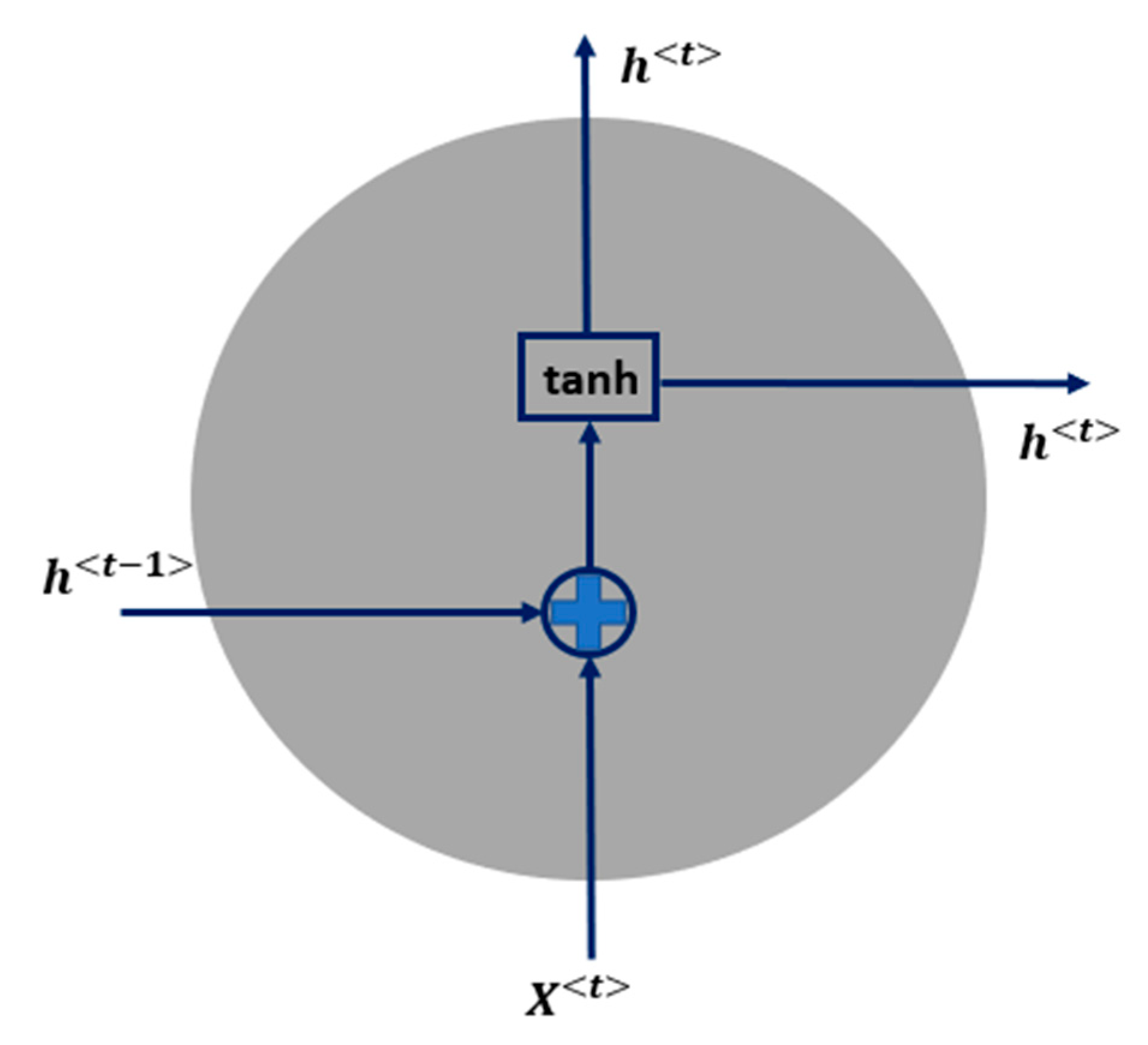
2.2. Architectures of RNN

Different types of RNN architectures could be trained, depending on the needs of the concrete problems, such as one-to-many for music generation [38], many-to-one for sentiment classification [39], sequence-to-sequence for machine translation [40], etc. With regards to the type of sequence-to-sequence, it can be further classified into subgroups, according to the lengths of input and output of the model. In this paper, the following notations are used: encoder–decoder architecture for scenarios, where the lengths of the input and output are not the same; many-to-many architecture for scenarios, where the lengths of the input and output are the same. In this work, traffic noise is the output of the model and multiple traffic feature variables are the inputs of the model. At each time step, the input traffic features are expected to predict a corresponding output traffic noise level. This problem can be formulated by following three different architectures as illustrated in Figure 5, where n_steps is the length of the sequence, m is the number of training samples, n is the number of feature variables. Please be aware that the grey round-shape nodes in different layers inside Figure 5 represent the recurrent units as discussed above, which could be simple RNN, LSTM or GRU.

The traffic noise modelling with the Blansko dataset can be constructed as a many-to-one problem (Figure 5a), when vectorizing each single output of a sequence, so that they can be treated as elements of one vector, corresponding to different time steps. However, in this way, the advantage of recurrent neural network for handling time series data is not thoroughly exploited, because the consideration of time dimension is discarded, due to vectorization. The problem can also be structured as a many-to-many architecture (Figure 5b). This is the most intuitive and intrinsic way to describe this problem. At each time step, along with the input feature variables, a corresponding traffic noise output is expected. The length of the output is equal to the length of the input. On the other hand, although encoder–decoder architecture is a general solution to problems, where the lengths of output and input are not equal, it can be indeed also applied to problems, where the length of output and input equals each other (Figure 5c), namely to this problem of Blansko data modelling. Different from many-to-many architecture, in the encoder–decoder architecture, only the hidden state from last time step of a recurrent layer will be sent to next layer [41]. This allows the applicability of encoder–decoder architecture to problems, where the lengths of input and output of the sequence are not equal.

2.3. Model Evaluation Metrics

To evaluate and compare the RNN models, following evaluation metrics are applied. The coefficient of determination, R², is a proportion of explained variance of the model and the total variance of the data. The value of R² is usually between 0 and 1. An R² of 0 means a bad fit and 1 indicates a perfect fit, meaning that the model can explain 100% variance of the data. Mathematically, R² can be expressed as:

$$R^2(y_i,\widehat{y})=\frac{ESS}{TSS}=1-\frac{RSS}{TSS},$$

(13)

$$RSS={\displaystyle \sum {(y_i-\widehat{y})}^2},$$

(14)

$$ESS={\displaystyle \sum {(\widehat{y}-\overline{y})}^2},$$

(15)

$$TSS={\displaystyle \sum {(y_i-\overline{y})}^2},$$

(16)

where $\widehat{y}$ is the predicted value, and $y_i$ is the true value, $\overline{y}$ is the average of the true value $y_i$. Total sum of squares (TSS) is the summation of residual sum of squares (RSS) and estimation sum of squares (ESS). Although R² is a very common evaluation metric for regression tasks, it has some drawbacks, namely, the R² value always increases when the number of variables increases. Hence, adjusted R² has been introduced, which imposes a penalty for adding additional explanatory variables and only increases when a significant variable is added. The equation of adjusted R² is shown below:

$$R^2{}_{adj}(y_i,\widehat{y})=1-\frac{(1-R^2)\times (n-1)}{n-k-1},$$

(17)

where n is the number of observations, and k is the number of features. Apart from R² and adjusted R², mean squared error (MSE), root mean squared error (RMSE), mean absolute error (MAE) and mean absolute percentage error (MAPE) are also used in this work for model evaluation and comparison. MSE measures the average of the squares of errors. RMSE is the square root of MSE. MAE is a measure of the average of the absolute errors. MAPE measures the accuracy as an average percentage of the absolute errors divided by true values. The corresponding mathematical expressions could be found below:

$$MSE=\frac{1}{n}{\displaystyle \sum _{i=0}^{n-1}{(y_i-\widehat{y_i})}^2},$$

(18)

$$RMSE=\sqrt{\frac{{\displaystyle \sum _{i=0}^{n-1}{(y_i-\widehat{y_i})}^2}}{n}},$$

(19)

$$MAE=\frac{1}{n}{\displaystyle \sum _{i=0}^{n-1}\left|y_i-\widehat{y_i}\right|},$$

(20)

$$MAPE=\frac{1}{n}{\displaystyle \sum _{i=0}^{n-1}\left|\frac{y_i-\widehat{y_i}}{y_i}\right|},$$

(21)

where n is number of observations, ${\widehat{y}}_i$ is the predicted value, and $y_i$ is the true value.

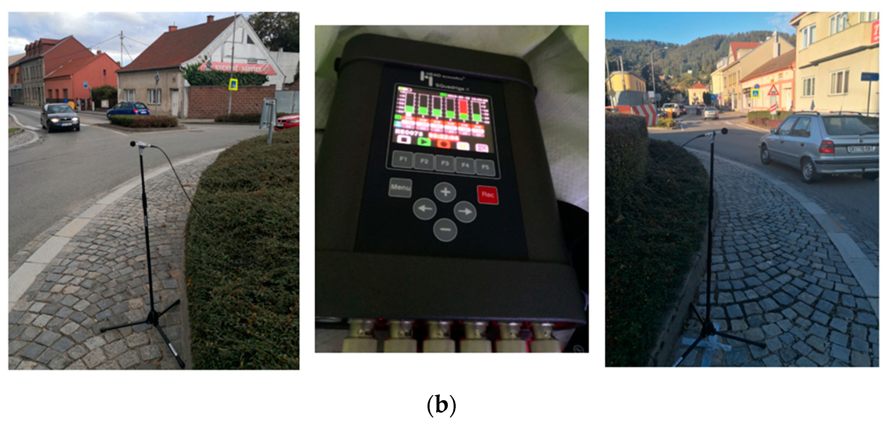
2.4. Experiment Setup and Data Acquisition

In this study, the data were collected near the town center in Blansko, Czech Republic, by video recording and audio recording over a roundabout (Figure 6). The roundabout has an inner diameter about 23.5 m and outer diameter about 38.2 m. The video recording was performed at the same time as the audio recording. A Hikvision IP camera, with a framerate of 30 fps, was installed and fixed on the roof of a 12-floor high building at the roundabout. The recording was performed over two days, with a total duration of around 9 h.

The audio recording was performed simultaneously while video recording. Five calibrated measurement microphones were standing at different locations of the roundabout at a height of 1.2 m above the ground, as shown in Figure 6 and Figure 7a. The five microphones were connected to different channels of the same recording device, Head acoustics SQuadriga II, with a sampling rate of 48 KHz (Figure 7b). All five microphones recorded simultaneously the traffic noise from the whole roundabout area. The technical details of the audio and video recording devices are listed in

Table 1. Technical details of recording devices: (a) info of audio and video recorders: (b) info of microphones.

(a)
	Device Model	Sampling Rate	Number of Channels
Audio Recording	SQuadriga II	48 KHz	10 (6 × Line/ICP In, BHS In (2-channel), 2 × Pulse In)
Video Recording	Hikvision IP camera	30 fps	N.A.
(b)
Microphones	Frequency Response	Sensitivity (mV/Pa)	Max. Peak SPL (dB)
Mic3	0.02–4 KHz (±0.5 dB) 4–20 KHz (±1.5 dB)	51.3	130
Mic5		51.0
Mic6		51.6
Mic7		51.9
Mic8		52.0

.

The audio and video data were synchronized, according to the local network time, since both the obtained audio data and video data had local time tags. The camera and audio recorder were synchronized with Central European Time. The total extracted audio and video recordings have the same starting and ending time, as indicated in

Table 2. The extracted recording times.

Date	Start	End	Total Duration
Day 1 (30 September 2019)	16:43 p.m.	20:32 p.m.	3 h 49 min
Day 2 (1 October 2019)	06:34 a.m.	11:48 a.m.	5 h 14 min
Day 1 + Day 2	-	-	9 h 3 min

.

Although the whole dataset is based on a recording of two half-days, this work focuses on the methodology of applying recurrent neural network for traffic noise modelling, for which the obtained dataset is sufficient. In future research, a longer and bigger experimental campaign is needed, covering more traffic scenarios such as different weather conditions, different road surfaces, different seasons, etc., in order to generalize the model.

2.5. Data Pre-Processing

2.5.1. Video Data Pre-Processing

The numeric video data, containing individual vehicle trajectories, was purchased from DataFromSky, a computer vision company, processing traffic videos. The individual vehicle trajectories were detected as shown in Figure 8. At each time step, the vehicle information, such as vehicle ID, vehicle type, vehicle location (GPS in UTM), vehicle instantaneous speed and acceleration/deceleration, were extracted from the raw video. In terms of vehicle type, we pre-defined the vehicle categories, according to the shape and dimension, and classified them into six categories, including motorcycle, small car, car, medium vehicle, heavy vehicle and bus. No engine information was taken into account, which could be improved in future work.

Based on the GPS information of each vehicle and each microphone, the distance between the sound source and receiver could be calculated, namely the instantaneous distances between each vehicle and each microphone.

2.5.2. Traffic Features Generation

To train a supervised machine-learning model, the input variables and output variable should be well defined in advance. In this specific problem, the traffic features are the input variables, and the corresponding traffic noise is the output variable. The next critical task is to convert the individual vehicle trajectory into traffic features, because the obtained noise level at each time step is contributed by the traffic as a whole. Two methods are proposed to represent the traffic features: statistic representation and histogram representation.

The initial individual vehicle trajectory data were in the order of vehicle ID. The whole dataset is re-ordered to time domain, at the time window of 1, 5, 9, 15 and 46 s, respectively. It takes around 10 to 15 s for one vehicle from driving in the roundabout to leaving the roundabout, when the traffic is flowing fluently. At each time step, all the individual vehicle features, such as speed, acceleration, deceleration, distance to receivers and vehicle category can be aligned together in different lists, as shown below in

Table 3. Illustration of raw data frame reorganized in time order.

Raw Data Frame		Vehicle Speed (km/h)	Vehicle Acceleration (m/s2)	Vehicle Deceleration (m/s2)	Vehicle Distance to Mic3 (m)	Vehicle Category
Sample1	Time step1	[0.0058, 0.0034, 0.0033, 0.0043, 34.35, 31.57, 0.084, 31.61, 0.29, 8.01, 44.59, 0.0, 0.0, 27.83, 4.56, 31.02, 24.72, 31.22]	[0.0005, 0.0012, 0.0008, 0.004, 0.0, 0.0, 0.014, 0.81, 0.13, 1.89, 0.0, 0.0, 0.0, 8.42, 0.018, 3.29, 0.38, 0.0]	[0.0, 0.0, 0.0, 0.0, 3.26, 2.56, 0.0, 0.0, 0.0, 0.0, 2.12, 0.0, 0.0, 0.0, 0.0, 0.0, 0.0, 0.26]	[39.08, 23.87, 22.70, 22.92, 68.57, 45.45, 55.99, 29.38, 46.05, 27.55, 53.53, 45.70, 22.82, 75.29, 47.44, 70.34, 94.37, 70.40]	[“car”, “car”, “car”, “car”, “car”, “car”, “car”, “car”, “car”, “heavy vehicle”, “car”, “car”, “car”, “car”, “car”, “car”, “car”, “small car”]
…	…	…	…	…	…	…
Sample800	Time step800	[33.61, 22.82, 17.68]	[1.44, 1.18, 1.19]	[0.0, 0.0, 0.0]	[41.69, 30.96, 30.01]	[“car”, “car”, “car”]
…	…	…	…	…	…	…

.

However, at different time steps, these data lists have different sizes, because the traffic recorded by the camera changes dynamically with time. Therefore, further feature variables are extracted from these data, in order to generate uniform data size, which can be used as input for training machine-learning model. Statistic representation and histogram representation are applied and compared, respectively. With statistic methods, summary statistics are extracted from each data list. Hence, the data distribution of each feature—speed, acceleration, deceleration, distance to microphone—is converted to its mean, min, max, standard deviation, median, range, mid-point, skewness and kurtosis. In terms of mean speed, both time mean speed and space mean speed are calculated. With regards to those lists of vehicle category, at each time step the number of vehicles is counted, equal to the size of the list, the proportions of each vehicle category are calculated. As a result, a total of 44 features have been generated, which can be observed below in

Table 4. The input variables of the machine-learning model.

Features Representing Individual Vehicle (Raw Data)	Input Variables for Machine-Learning Model (after Preprocessing)
Vehicle category	[traffic volume, ratio of motorcycle, ratio of medium vehicle, ratio of heavy vehicle, ratio of bus, ratio of car, ratio of small car]
Vehicle speed	[arithmetic mean, harmonic mean, min, max, median, range, mid-point, standard deviation, skewness, kurtosis]
Vehicle acceleration	[arithmetic mean, min, max, median, range, mid-point, standard deviation, skewness, kurtosis]
Vehicle deceleration	[arithmetic mean, min, max, median, range, mid-point, standard deviation, skewness, kurtosis]
Vehicle distance to mics	[arithmetic mean, min, max, median, range, mid-point, standard deviation, skewness, kurtosis]

:

As shown in Table 4, the left column corresponds to the raw data, while the right column shows the transformed results from raw data, and they are the final forty-four input variables used for the machine-learning model. With the histogram method, the width of bins and number of bins are pre-defined. The extracted features are the counts of instances falling in each bin. The number of features is the number of bins. Due to the spread of the data, more bins have to be predefined, in order to cover all the data. As a consequence, a total of 391 features have been generated. Compared to statistic representation, histogram representation results in a high dimension and data sparsity. Besides, the data are discretized and have lost the physical meaning, as they are simply the counts of instances falling in that bin.

2.5.3. Audio Data Pre-Processing

With regards to the audio data, the root mean square (RMS) sound pressure was extracted from the raw audio file, at the time window of 1, 5, 9, 15 and 46 s, respectively, corresponding to the video data. The sound pressure was then transformed to sound pressure level (SPL dB), with the equation below:

$$SPL=20{\log }_{10}(\frac{p}{2\times {10}^{-5}})dB,$$

(22)

where $p$ is the RMS sound pressure, $2\times {10}^{-5}$ is the reference sound pressure in air.

In order to have more data for model training, data from all five microphones from both days were used, since they delivered different messages (Figure 9), although the microphones were physically not that far away from each other at the roundabout.

As shown in Figure 9, the recorded SPL curves from the five microphones from each day indicate a similar tendency, since the microphones were located at the same roundabout. However, due to the spatial distance, the shift in the peak values could still be observed, because the recorded SPL from a specific microphone at a certain time step would be dominated by the loud vehicle nearby. Due to the difference in the carried messages of different microphones, it makes sense to mix and use all these data for the model training. In this regard, each microphone data is further aligned with the data of generated traffic features at each time step. For different microphones, at each time step, the paired traffic features are almost the same except for distance-related features, because the five microphones were standing in different locations.

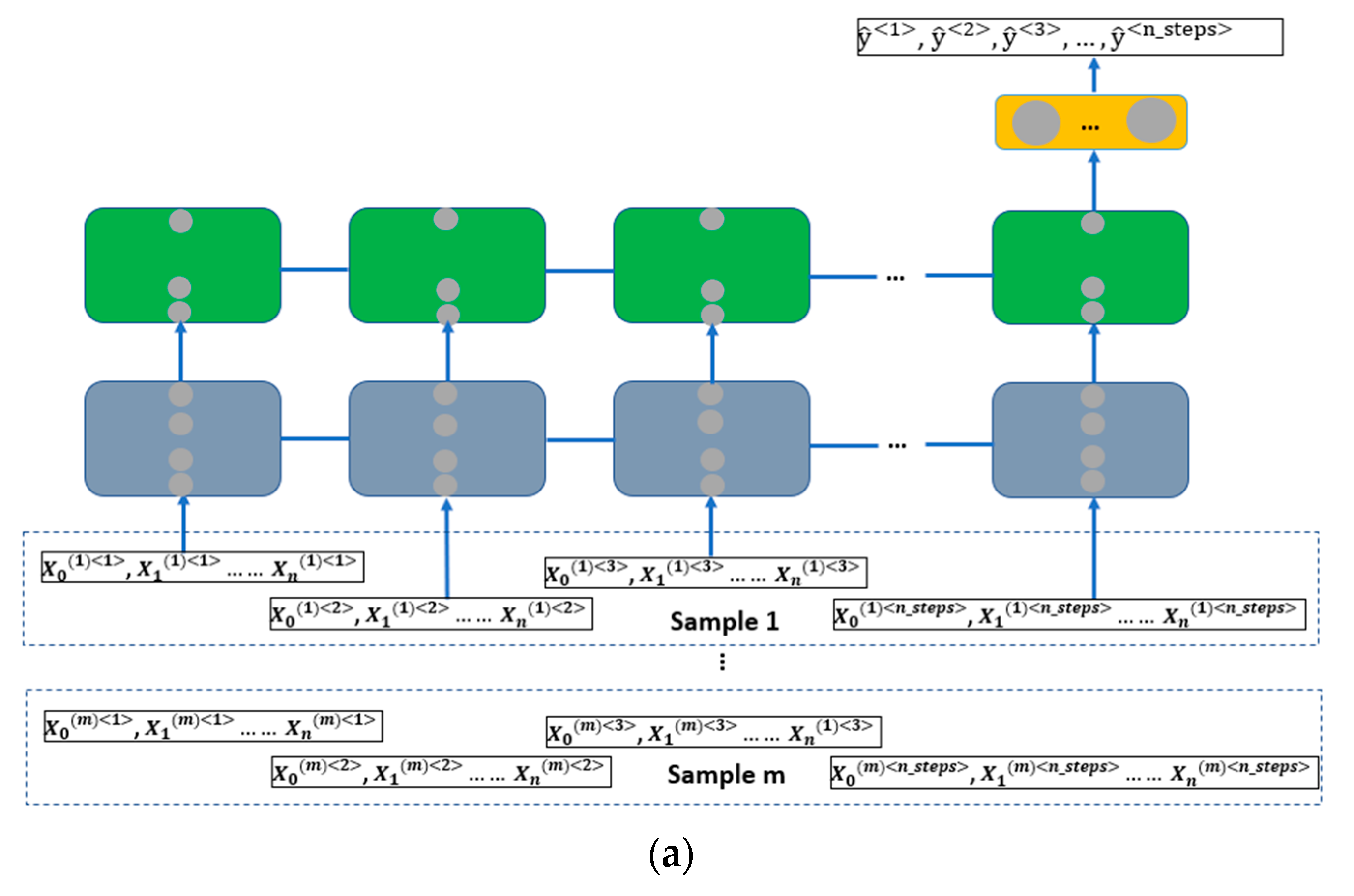
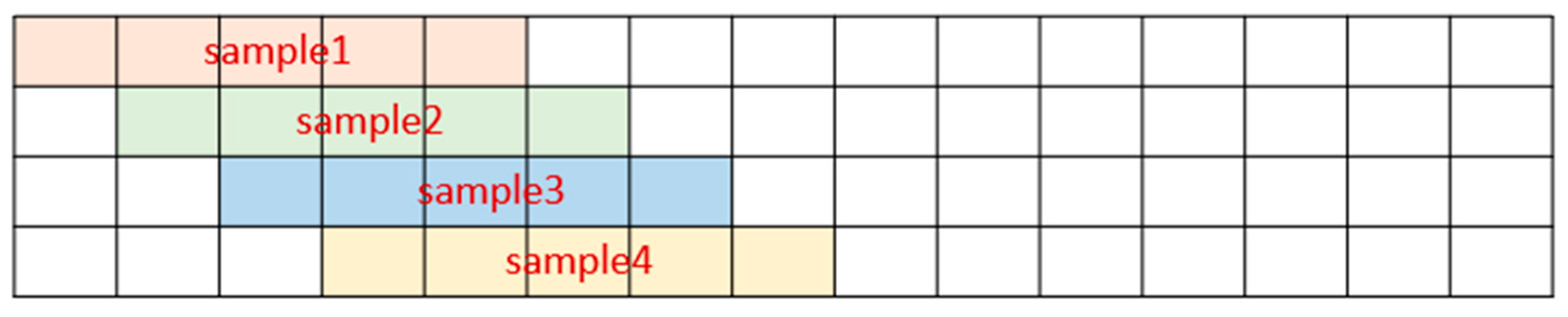
2.5.4. RNN Training Samples Generation

In conventional machine-learning algorithms, each training sample is a vector, made of feature and target variables. Different from that, in a recurrent neural network, each training sample is a sequence (tensor), consisting of multiple vectors. The additional dimension is time domain. The length of the sequence, n_steps, is a hyperparameter of RNN. In this work, different values of n_steps are compared.

The total data are divided into training data, validation data and testing data, for achieving an unbiased result. In order to increase the training data size, each training sample is generated with overlap with adjacent samples. The same method was applied to the generation of the validation samples (Figure 10). Each testing sample is generated without overlap (Figure 11), so that the final evaluation metric can be calculated on each single point of testing data only once. Please notice, to make it clearly illustrated, n_steps = 5 is used in both Figure 10 and Figure 11, which does not stand for the final tuned value of this hyperparameter.

2.5.5. Leave One Subject out Cross-Validation

Leave-one-subject-out cross-validation has been applied, in order to achieve a robust result. As shown in

Table 5. Leave-one-subject-out cross-validation (n_steps = 30).

	Samples for Model Training		Model Evaluation
	Training Data	Validation Data	Testing Data
Data Shape	(6276, 30, 44)	(2092, 30, 44)	(70, 30, 44)
1st iteration	Mic3, 6, 7	Mic5	Mic8
2nd iteration	Mic3, 6, 8	Mic5	Mic7
3rd iteration	Mic3, 7, 8	Mic5	Mic6
4th iteration	Mic6, 7, 8	Mic3	Mic5
5th iteration	Mic6, 7, 8	Mic5	Mic3

, at each iteration, one microphone data is used as the testing data, and the remaining data are used as training data, until all the microphones have been used once as testing data. Therefore, five microphones lead to five iterations of each training process. The final evaluation will be averaged over the five iterations.

The whole process is called leave-one-subject-out cross-validation. The subject refers to different microphones here. Leave-one-subject-out cross-validation makes sure that the model does not have subject bias [42].

2.5.6. Data Scaling

Each variable has a different physical meaning, with different ranges and spreads in scales. To use them directly for model training will slow down the convergence of the learning process. It also increases the chance of becoming stuck in the local minimum, when calculating the optimal weights. Hence, it is necessary to standardize the feature variables to obtain a uniform scale. The output variable has also been scaled, in order to match the scale of the activation function of the output layer in the neural networks.

3. Results and Discussion

This work was performed in Python, with Keras API, running on top of TensorFlow. A development environment with support of GPU, NVIDIA GeForce MX150, providing accelerated high performance, was adapted for the whole simulation.

The work flow of this project is illustrated in Figure 12. The model performances were compared based on different time steps, different methods of representing traffic features, different architectures, different recurrent units and different hyperparameters such as sequence length (n_steps) in this work. The red highlighted path in Figure 12 indicated the final selected model, which achieved the best performance.

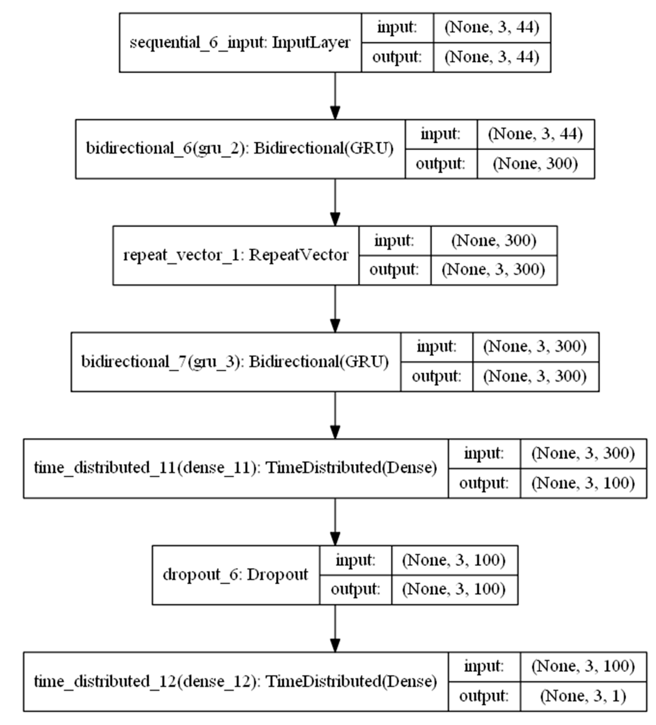
3.1. Development of RNN

As mentioned above, the problem in this paper can be constructed with three different architectures: many-to-one, many-to-many and encoder–decoder. At each time step, along with the input traffic feature variables, a corresponding traffic noise output is expected. All these three architectures are trained with Blansko data, and corresponding model performances have been compared in this paper. After some basic tuning, such as number of layers and number of neurons, the trained models based on the three different architectures are obtained, as shown in Figure 13, Figure 14 and Figure 15. Bidirectional recurrent neural network (BRNN) is applied, which is an extension of the conventional RNN [43]. BRNN can improve the model performance, because BRNN trains the model not only on the input sequence, but also on the reversed copy of the input sequence. Therefore, BRNN obtains additional context for predicting the current state by using the information from both the past and the future.

First model, based on Architecture 1, many-to-one, is stacked RNN network (Figure 13), with two bi-directional RNN layers and one fully connected dense layer, which is the output layer with a single neuron. The model output is a vector with the same length as the time steps of the sample sequence, n_steps.

Second model, based on Architecture 2, many-to-many, has one bi-directional RNN layer and two fully connected dense layers including one output layer with a single neuron at each time step (Figure 14). Each of the two dense layers is wrapped by TimeDistributed API. TimeDistributed API applies the same operation to every temporal slice of the 3D tensor.

The third model, based on Architecture 3, is an encoder–decoder network, where the encoder and decoder each consists of an RNN layer (Figure 15). Only the last output of the sequence from the encoder is sent to every temporal slice of the decoder, by RepeatVector API [44]. Two more fully connected dense layers were wrapped with TimeDistributed API, where one of them is output layer with single neuron, same as mentioned in Architecture 2.

Among all these three trained models, dropout was also applied, in order to avoid model overfitting.

3.2. Results Comparison on Different Architectures

The encoder–decoder architecture failed to achieve a good result when modelling the Blansko data with n_steps of 30; instead, it achieved the best performance when n_steps is set to 3. Otherwise, the network has to increase the complexity, such as adding more layers, more neurons or training for a longer time, in order to achieve a comparable performance to the other two architectures, which leads to a much higher computation cost. Therefore, the below demonstrated result based on encoder–decoder architecture was using n_steps of 3 (Figure 15 and Figure 16).

Figure 16 shows the result comparison of the models trained from these three architectures with testing data, in the aspects of prediction accuracy (Figure 16a) and computation efficiency (Figure 16b). It is noticeable that the prediction performances of Architecture 1 and 2 are very similar with an RMSE around 2.4 dB and an R² around 0.68, slightly better than the performance of Architecture 3 with an RMSE around 2.7 dB and an R² around 0.64, as shown in Figure 16a. However, as indicated in Figure 16b, the model training took a very long time with Architecture 1, almost 10 times longer computation time than Architecture 2; Architecture 1 trained 15 times more parameters than Architecture 2 by backpropagation, where the model based on Architecture 1 learned 590,430 parameters, and the model based on Architecture 2 learned 38,701 parameters. Architecture 3, in terms of both prediction accuracy and computation efficiency, does not have any privilege. Therefore, Architecture 2 was selected for training the recurrent neural network model.

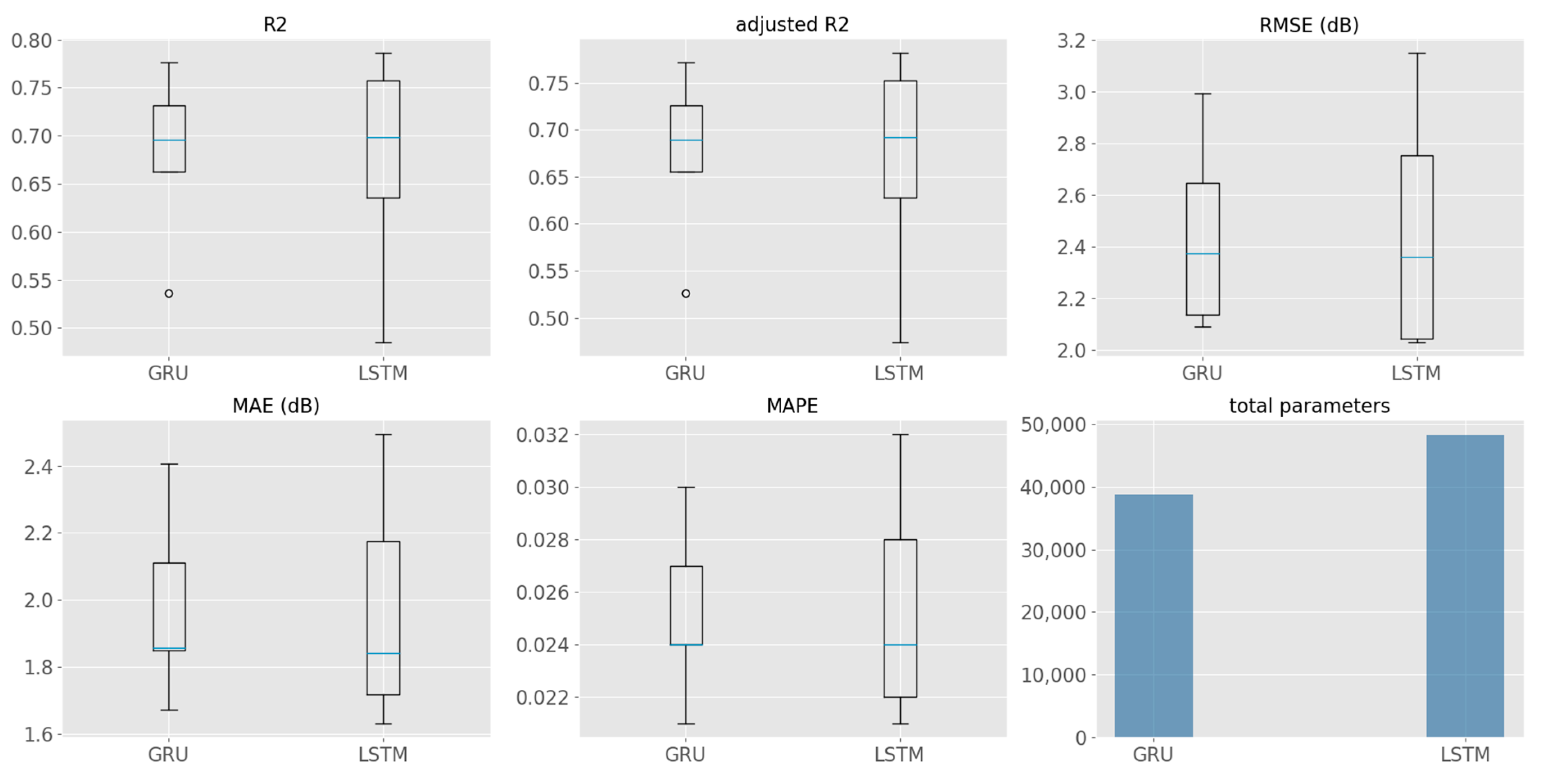
3.3. Results Comparison on Recurrent Units

GRU and LSTM were further compared. The performance comparison on GRU and LSTM with testing data are shown in Figure 17. The results were based on five iterations of cross-validation.

As indicated by the boxplots of Figure 17, it is clear to observe that the spread of LSTM in the results of different evaluation metrics is larger than GRU model, although the median and mean values of each evaluation metric, R², adjusted R², RMSE, MAE and MAPE, are similar to each other. With the same configuration of the network, 48,201 parameters need to be trained in LSTM, while only 38,701 parameters need to be trained in GRU. As mentioned at the beginning, the GRU model is the simplified version of LSTM. It is also proven here that there is no additional cost of model performance, when using GRU instead of LSTM for Blansko traffic noise data modelling. Hence, the GRU model, with Architecture 2 (many-to-many), is the finalized traffic noise model for Blansko dataset.

3.4. Model Hyperparameters Tuning

Different hyperparameters were also tuned during the whole model training process. Compared to conventional fully connected ANN, the RNN model has much more hyperparameters to tune. The final setting of the tuned hyperparameters can be found in

Table 6. Final GRU model’s hyperparameters.

Hyperparameter	Value
Number of layers	3 (one bidirectional GRU layer, two dense layers)
Number of neurons	50, 100, 1
Learning rate	0.0001
Batch size	256
Optimization algorithm	Adam
Dropout rate	0.4
Sequence length (n_steps)	30
Number of Epochs	143 (controlled by Keras Early Stopping)

.

A GRU model with three layers was finalized. Each layer has 50, 100 and 1 neuron, respectively. The learning rate determines the step size at each iteration when moving toward the minimum of loss function during the optimization process [45]. Therefore, it controls the speed at which the model learns. The learning rate was set to 0.0001 here. The batch size controls the number of training samples that are used for weights update at each iteration, which was finally fixed at 256. Adam was chosen as the optimization algorithm, which is an advanced method for stochastic optimization [46]. Dropout regularization was employed with a dropout rate of 0.4, in order to efficiently mitigate overfitting [47]. The number of epochs was not predefined. Instead, the duration of the training was configured by applying Keras EarlyStopping API, which enables us to compare the model performance between training data and validation data [44]. During the training process, the loss of training data and validation data will both sink along with the epochs. The training data loss will keep decreasing, as long as the training continues. However, the validation data loss will start to increase, when the model is overfitting. With the help of Keras EarlyStopping API, the model stops training, when the validation loss does not reduce any more, which helps to avoid model overfitting (Figure 18).

As shown in Figure 18, at Epoch 143, the model has stopped training, because validation data loss does not reduce any more.

3.5. Final Model Evaluation

The final model has been validated with testing data. A certain period of the prediction on each day can be observed in Figure 19.

It can be seen that the proposed model catches the tendency of the dynamic change of the real traffic noise level in a short time interval. When the sound level increases or decreases drastically, it is relatively difficult for the model to precisely estimate the noise peak values. This phenomenon is explainable with the statistical rule of regression toward the mean, which describes the model aims to predict the expected value, closer to the mean on the measurements [48].

Figure 20 illustrates the predicted SPL against the real SPL of the testing data (Figure 20a) and the distribution of the corresponding residuals (Figure 20b). In Figure 20a, it is clear to see that the predicted SPL values and the actual SPL values have a good fit around the red dashed reference line indicating the ideal case, where the predictions equal the ground truth. A mean of −0.509 dB and a standard deviation of 2.309 dB with a bell shape can be observed in the distribution of testing data residuals in Figure 20b.

The overall results after leave-one-subject-out cross-validation with GRU, many-to-many architecture, can be found in

Table 7. The evaluations on GRU model, Architecture 2, on testing data.

	R2	Adjusted R2	RMSE	MAE	MAPE
1st iteration	0.6953	0.6888	2.373	1.857	0.024
2nd iteration	0.6629	0.6557	2.648	2.111	0.027
3rd iteration	0.5359	0.526	2.993	2.406	0.030
4th iteration	0.7766	0.7718	2.09	1.673	0.021
5th iteration	0.7319	0.7262	2.136	1.848	0.024
Average	0.6805	0.6737	2.448	1.979	0.0252
Standard dev.	0.0816	0.0834	0.3371	0.2551	0.0031

.

As shown in Table 7, given 95% confidence interval, the model achieves an RMSE of 2.448 ± 0.67 dB and a MAE of 1.979 ± 0.51 dB.

The results of each iteration might slightly vary after multiple running, due to the random initialization of weights in neural networks. Besides, the used batch for updating the weights during one iteration through gradient descent is generated with random sampling techniques, which could also lead to a slight variation in the final result.

3.6. Comparison with CNOSSOS-EU Model

The obtained result from the GRU model has been further compared to the EU standard traffic noise model, the CNOSSOS model. The CNOSSOS model is expressed in octave bands in the frequency range from 125 to 4 KHz, for a reference speed of 70 km/h and a road surface of stone mastic asphalt and dense asphalt concrete. The vehicles are classified into four categories: light motor vehicles, medium heavy vehicles, heavy vehicles and powered two-wheelers [49]. Each vehicle is considered as a point source. The rolling noise sound power level and propulsion noise sound power level were calculated for each vehicle in the selected roundabout in Blansko over a time window of 15 s, same as the development of GRU model. The propagation part was calculated with CNOSSOS propagation formula, considering only the attenuation caused by geometric divergence. The standard parameters of the CNOSSOS model for all member states of the EU were used for the source emission and propagation calculations [50]. Compared to the ground truth values, the RMSE, MAE and MAPE of the CNOSSOS predicted values were calculated. The obtained result is shown below in

Table 8. The evaluations on the common noise assessment methods (CNOSSOS) model.

Testing Data	RMSE	MAE	MAPE
Mic3	6.357	4.902	0.063
Mic5	7.706	6.294	0.079
Mic6	7.494	6.121	0.077
Mic7	7.189	5.659	0.072
Mic8	6.967	5.539	0.071
Average	7.143	5.703	0.072
Standard dev.	0.467	0.489	0.006

:

As shown in Table 8, given the 95% confidence interval, the CNOSSOS model achieves an RMSE of 7.143 ± 0.93 dB and a MAE of 5.703 ± 0.98 dB, for traffic noise prediction with Blansko dataset. It turns out that the RMSE achieved by the GRU model is around 4.7 dB smaller than CNOSSOS model. The proposed GRU model outperforms CNOSSOS model for traffic noise short-term prediction.

4. Conclusions

In conclusion, we are stepping into the new data age, artificial intelligence is under the spotlight across different disciplines, due to its high capability of handling large datasets. In this paper, a recurrent neural network was applied to traffic noise prediction with multivariate traffic features as the predictors. The trained model could predict traffic noise according to the traffic scenario, instead of setting audio devices for traffic noise recording. Simple RNN, LSTM and GRU were introduced and compared in this paper. Different architectures of RNN were trained with the dataset, obtained from an urban roundabout in Blansko, CZ. As a result, the GRU model with many-to-many architecture was selected as the final model, due to its best performance in both prediction accuracy and computation efficiency, with an achieved RMSE of circa 2.4 ± 0.7 dB and a MAE of 2.0 ± 0.5 dB.

The excellent performance of the trained GRU model shows the great potential of applying GRU for traffic noise modelling in the short term. The traffic noise model can help policy makers and urban authorities to carry out different measures, such as speed limit, traffic volume control, new traffic infrastructure assessment, etc., in order to mitigate the noise pollution caused by road traffic. In additional, accurate short-term prediction catches the variations of the traffic noise over a short period, which can further contribute to traffic-noise-peak-caused annoyance studies.

In future research, the obtained GRU model will be generalized. The presented model is trained on the Blansko dataset and applicable in the selected roundabout. However, many other factors, such as road surface, surroundings, and meteorology, were not taken into account in this work, due to the lack of the relevant data. In order to overcome the limitations in obtaining very large datasets, data augmentation techniques such as the generative adversarial network (GAN) could be applied, which was developed by Ian Goodfellow and his colleagues in 2014 [51]. Additionally, a hybrid model by combining a machine-learning model and empirical or physical noise models could be further developed, in order to take advantage of the strengths from different types of traffic noise models and achieve model generalization. Last but not least, a longer experiment campaign is needed for obtaining more ground truth values and covering wider traffic scenarios and meteorology conditions, for validating the generalized model.

References

1. Hänninen, O.; Knol, A.; Jantunen, M.; Lim, T.; Conrad, A.; Rappolder, M.; Carrer, P.; Fanetti, A.; Kim, R.; Buekers, J.; et al. Environmental Burden of Disease in Europe: Assessing Nine Risk Factors in Six Countries. Environ. Health Perspect. 2014, 122, 439–446. [Google Scholar] [CrossRef] [Green Version]
2. Miloradović, D.; Glišović, J.; Lukić, J. Regulations on Road Vehicle Noise—Trends and Future Activities. Mob. Veh. Mech. 2017, 43, 57–72. [Google Scholar] [CrossRef] [Green Version]
3. Guarnaccia, C. EAgLE: Equivalent acoustic level estimator proposal. Sensors (Switzerland) 2020, 20, 701. [Google Scholar] [CrossRef] [PubMed] [Green Version]
4. Rey Gozalo, G.; Aumond, P.; Can, A. Variability in sound power levels: Implications for static and dynamic traffic models. Transp. Res. Part D Transp. Environ. 2020, 84. [Google Scholar] [CrossRef]
5. Guarnaccia, C.; Bandeira, J.; Coelho, M.C.; Fernandes, P.; Teixeira, J.; Ioannidis, G.; Quartieri, J. Statistical and semi-dynamical road traffic noise models comparison with field measurements. AIP Conf. Proc. 2018, 1982. [Google Scholar] [CrossRef]
6. Golmohammadi, R.; Abbaspour, M.; Nassiri, P.; Mahjub, H. Road traffic noise model. J. Res. Health Sci. 2007, 7, 13–17. [Google Scholar]
7. Steele, C. Critical review of some traffic noise prediction models. Appl. Acoust. 2001, 62, 271–287. [Google Scholar] [CrossRef]
8. Guarnaccia, C.; Lenza, T.L.L.; Mastorakis, N.E.; Quartieri, J. A comparison between traffic noise experimental data and predictive models results. Int. J. Mech. 2011, 5, 379–386. [Google Scholar]
9. Quartieri, J.; Mastorakis, N.E.; Iannone, G.; Guarnaccia, C.; Ambrosio, S.D.; Troisi, A.; Lenza, T.L.L. A Review of Traffic Noise Predictive Noise Models. In Proceedings of the Recent Advances in Applied and Theoretical Mechanics, 5th WSEAS International Conference on Applied and Theoretical Mechanics (MECHANICS’09), Puerto De La Cruz, Tenerife, Canary Islands, Spain, 14–16 December 2009; pp. 72–80. [Google Scholar]
10. Garg, N.; Maji, S. A critical review of principal traffic noise models: Strategies and implications. Environ. Impact Assess. Rev. 2014, 46, 68–81. [Google Scholar] [CrossRef]
11. Petrovici, C.; Tomozei, F.; Nedeff, O. Irimia, and M. Panainte-Lehadus, A. Review on the Road Traffic Noise Assessment. J. Eng. Stud. Res. 2016, 22, 81–89. [Google Scholar]
12. Bakowski, A.; Dekýš, V.; Radziszewski, L.; Skrobacki, Z. Validation of traffic noise models. AIP Conf. Proc. 2019, 2077. [Google Scholar] [CrossRef]
13. Huang, K.; Fan, Y.; Dai, L. A nested ensemble filtering approach for parameter estimation and uncertainty quantification of traffic noise models. Appl. Sci. 2020, 10, 204. [Google Scholar] [CrossRef] [Green Version]
14. Dutilleux, G.; Soldano, B. Matching directive 2015/996/EC (CNOSSOS-EU) and the French emission model for road pavements. In Proceedings of the Euronoise, Heraklion-Crete, Greece, 27–31 May 2019; pp. 1213–1218. [Google Scholar]
15. Kumar, K.; Ledoux, H.; Schmidt, R.; Verheij, T.; Stoter, J. A harmonized data model for noise simulation in the EU. ISPRS Int. J. Geo-Information 2020, 9, 121. [Google Scholar] [CrossRef] [Green Version]
16. Andrzej, B.; Leszek, R. Simulation and Assessments of Urban Traffic Noise by Statistical Measurands using mPa or dB(A) Units. Terotechnology XI 2020, 17, 108–113. [Google Scholar]
17. Hamad, K.; Ali Khalil, M.; Shanableh, A. Modeling roadway traffic noise in a hot climate using artificial neural networks. Transp. Res. Part D Transp. Environ. 2017, 53, 161–177. [Google Scholar] [CrossRef]
18. Zhang, X.; Zhao, M.; Dong, R. Time-series prediction of environmental noise for urban iot based on long short-term memory recurrent neural network. Appl. Sci. 2020, 10, 1144. [Google Scholar] [CrossRef] [Green Version]
19. Navarro, J.M.; Martínez-España, R.; Bueno-Crespo, A.; Martínez, R.; Cecilia, J.M. Sound levels forecasting in an acoustic sensor network using a deep neural network. Sensors 2020, 20, 903. [Google Scholar] [CrossRef] [PubMed] [Green Version]
20. Mansourkhaki, A.; Berangi, M.; Haghiri, M.; Haghani, M. A neural network noise prediction model for Tehran urban roads. J. Environ. Eng. Landsc. Manag. 2018, 26, 88–97. [Google Scholar] [CrossRef]
21. Givargis, S.; Karimi, H. A basic neural traffic noise prediction model for Tehran’s roads. J. Environ. Manag. 2010, 91, 2529–2534. [Google Scholar] [CrossRef] [PubMed]
22. Freitas, E.; Tinoco, J.; Soares, F.; Costa, J.; Cortez, P.; Pereira, P. Modelling Tyre-Road Noise with Data Mining Techniques. Arch. Acoust. 2015, 40, 547–560. [Google Scholar] [CrossRef] [Green Version]
23. Nourani, V.; Gökçekuş, H.; Umar, I.K. Artificial intelligence based ensemble model for prediction of vehicular traffic noise. Environ. Res. 2020, 180, 108852. [Google Scholar] [CrossRef]
24. Xu, D.; Wei, C.; Peng, P.; Xuan, Q.; Guo, H. GE-GAN: A novel deep learning framework for road traffic state estimation. Transp. Res. Part C Emerg. Technol. 2020, 117, 102635. [Google Scholar] [CrossRef]
25. Behrendt, K.; Novak, L.; Botros, R. A deep learning approach to traffic lights: Detection, tracking, and classification. In Proceedings of the 2017 IEEE International Conference on Robotics and Automation (ICRA), Singapore, 29 May–3 June 2017; pp. 1370–1377. [Google Scholar]
26. Yu, R.; Li, Y.; Shahabi, C.; Demiryurek, U.; Liu, Y. Deep learning: A generic approach for extreme condition traffic forecasting. In Proceedings of the 2017 SIAM International Conference on Data Mining (SDM), Houston, TX, USA, 27–29 April 2017; pp. 777–785. [Google Scholar]
27. Al-Qizwini, M.; Barjasteh, I.; Al-Qassab, H.; Radha, H. Deep learning algorithm for autonomous driving using googlenet. In Proceedings of the IEEE Intelligent Vehicles Symposium (IV), Los Angeles, CA, USA, 11–14 June2017; pp. 89–96. [Google Scholar]
28. Bravo-Moncayo, L.; Lucio-Naranjo, J.; Chávez, M.; Pavón-García, I.; Garzón, C. A machine learning approach for traffic-noise annoyance assessment. Appl. Acoust. 2019, 156, 262–270. [Google Scholar] [CrossRef]
29. Socoró, J.C.; Alías, F.; Alsina-Pagès, R.M. An anomalous noise events detector for dynamic road traffic noise mapping in real-life urban and suburban environments. Sensors 2017, 17, 2323. [Google Scholar] [CrossRef] [PubMed]
30. Shrestha, M.B.; Bhatta, G.R. Selecting appropriate methodological framework for time series data analysis. J. Financ. Data Sci. 2018, 4, 71–89. [Google Scholar] [CrossRef]
31. Medsker, L.; Jain, L.C. (Eds.) Recurrent Neural Networks: Design and Applications; CRC Press: Boca Raton, FL, USA, 1999. [Google Scholar]
32. Shewalkar, A.; Nyavanandi, D.; Ludwig, S.A. Performance Evaluation of Deep neural networks Applied to Speech Recognition: Rnn, LSTM and GRU. J. Artif. Intell. Soft Comput. Res. 2019, 9, 235–245. [Google Scholar] [CrossRef] [Green Version]
33. Rumelhart, D.E.; Hinton, G.E.; Williams, R.J. Learning representations by back-propagating errors. Nature 1986, 323, 533–536. [Google Scholar] [CrossRef]
34. McClelland, J.L.; Rumelhart, D.E.; PDP Research Group. Parallel Distributed Processing; IEEE: Wakefield, MA, USA, 1988; Volume 1. [Google Scholar]
35. Mozer, M.C. A focused backpropagation algorithm for temporal pattern recognition. In Backpropagation: Theory, Architectures, and Applications; Lawrence Erlbaum Associates: Hillsdale, NJ, USA, 1995; pp. 137–169. [Google Scholar]
36. Hochreiter, S.; Schmidhuber, J. Long Short-Term Memory. Neural Comput. 1997, 9, 1735–1780. [Google Scholar] [CrossRef]
37. Cho, K.; Van Merriënboer, B.; Gulcehre, C.; Bahdanau, D.; Bougares, F.; Schwenk, H.; Bengio, Y. Learning phrase representations using RNN encoder-decoder for statistical machine translation. In Proceedings of the EMNLP 2014—2014 Conference on Empirical Methods in Natural Language Processing, Doha, Qatar, 25–29 October 2014. [Google Scholar]
38. Briot, J.P.; Pachet, F. Deep learning for music generation: Challenges and directions. Neural Comput. Appl. 2020, 32, 981–993. [Google Scholar] [CrossRef] [Green Version]
39. Seo, S.; Kim, C.; Kim, H.; Mo, K.; Kang, P. Comparative Study of Deep Learning-Based Sentiment Classification. IEEE Access 2020, 8, 6861–6875. [Google Scholar] [CrossRef]
40. Luong, M.T.; Le, Q.V.; Sutskever, I.; Vinyals, O.; Kaiser, L. Multi-task sequence to sequence learning. arXiv 2015, arXiv:1511.06114. [Google Scholar]
41. Park, S.H.; Kim, B.; Kang, C.M.; Chung, C.C.; Choi, J.W. Sequence-to-Sequence Prediction of Vehicle Trajectory via LSTM Encoder-Decoder Architecture. In Proceedings of the 2018 IEEE Intelligent Vehicles Symposium (IV), Changshu, China, 26–30 June 2018; pp. 1672–1678. [Google Scholar]
42. Gholamiangonabadi, D.; Kiselov, N.; Grolinger, K. Deep Neural Networks for Human Activity Recognition With Wearable Sensors: For Model Selection. IEEE Access 2020, 8, 133982–133994. [Google Scholar] [CrossRef]
43. Schuster, M.; Paliwal, K.K. Bidirectional recurrent neural networks. IEEE Trans. Signal Process. 1997, 45, 2673–2681. [Google Scholar] [CrossRef] [Green Version]
44. Géron, A. Hands-On Machine Learning with Scikit-Learn, Keras, and TensorFlow: Concepts, Tools, and Techniques to Build Intelligent Systems; O’Reilly Media: Newton, MA, USA, 2019. [Google Scholar]
45. Murphy, K.P. Machine Learning: A Probabilistic Perspective; MIT Press: Cambridge, MA, USA, 2012; ISBN 978-0-262-01802-9. [Google Scholar]
46. Kingma, D.P.; Ba, J. Adam: A Method for Stochastic Optimization. arXiv 2014, arXiv:1412.6980. [Google Scholar]
47. Srivastava, N.; Hinton, G.; Krizhevsky, A.; Sutskever, I.; Salakhutdinov, R. Dropout: A Simple Way to Prevent Neural Networks from Overfitting. J. Mach. Learn. Res. 2014, 15, 1929–1958. [Google Scholar]
48. Everitt, B.; Skrondal, A. The Cambridge Dictionary of Statistics; Cambridge University Press: Cambridge, UK, 2002; ISBN 0-521-81099-X. [Google Scholar]
49. Kephalopoulos, S.; Paviotti, M.; Ledee, F.A. Common Noise Assessment Methods in Europe (CNOSSOS-EU); Publications Office of the European Union: Luxembourg, 2012; ISBN 9789279252815. [Google Scholar]
50. Kok, A.; van Beek, A. Amendments for CNOSSOS-EU. RIVM Rep. 2019, 23, 101–107. [Google Scholar]
51. Goodfellow, I.J.; Pouget-Abadie, J.; Mirza, M.; Xu, B.; Warde-Farley, D.; Ozair, S.; Courville, A.; Bengio, Y. Generative adversarial nets. Adv. Neural Inf. Process. Syst. 2014, 27, 2672–2680. [Google Scholar]
Figure 1. Recurrent neural network (RNN) architecture: recurrent layer with a feedback loop, indicating the additional time dimension after unfolding it.
Applsci 11 02714 g001
Figure 2. Illustration of simple RNN unit, having a simple structure without gate.
Applsci 11 02714 g002
Figure 3. Illustration of long short-term memory (LSTM) unit, having three gates and a memory cell state.
Applsci 11 02714 g003
Figure 4. Illustration of gated recurrent unit (GRU) unit, having two gates without dedicated memory cell state.
Applsci 11 02714 g004
Figure 5. The appropriate RNN model architectures for traffic noise modelling, based on Blansko data: (a) Many-to-one architecture: sequence input and single output. (b) Many-to-many architecture: synced sequence input and sequence output. (c) Encoder–decoder architecture: sequence input and sequence output (not necessary to be synced).
Applsci 11 02714 g005aApplsci 11 02714 g005b
Figure 6. The camera scene over the roundabout, 3, 5, 6, 7, 8 refer to the locations of the microphones.
Applsci 11 02714 g006
Figure 7. The audio recording setup: (a) indication of microphone locations; (b) picture of instruments used for audio recording.
Applsci 11 02714 g007aApplsci 11 02714 g007b
Figure 8. Video pre-processing and vehicle trajectory detection.
Applsci 11 02714 g008
Figure 9. Extracted SPL every other five minutes during the two days from different microphones: (a) SPL every other five minutes from day 1; (b) SPL every other five minutes from day 2.
Applsci 11 02714 g009
Figure 10. An example illustration of generating training samples and validation samples for data augmentation (n_steps = 5).
Applsci 11 02714 g010
Figure 11. An example illustration of generating testing samples (n_steps = 5).
Applsci 11 02714 g011
Figure 12. Work flow in the traffic noise modelling with Blansko data.
Applsci 11 02714 g012
Figure 13. Model based on Architecture 1: many-to-one architecture.
Applsci 11 02714 g013
Figure 14. Model based on Architecture 2: many-to-many architecture.
Applsci 11 02714 g014
Figure 15. Model based on Architecture 3: encoder–decoder architecture.
Applsci 11 02714 g015
Figure 16. GRU model performance comparison on different architectures: (a) the accuracy comparison on different architectures; (b) the computation cost comparison on different architectures.
Applsci 11 02714 g016
Figure 17. GRU and LSTM performance comparison, described by prediction accuracy indicators (boxplots) and computation cost indicator (bar plot).
Applsci 11 02714 g017
Figure 18. Model learning curve showing the reduction in training data error and validation data error over the GRU model training process.
Applsci 11 02714 g018
Figure 19. Illustrations of captured and estimated SPL data over a selected time on each day (data from Mic 8): (a) model prediction over a selected time on the first day; (b) model prediction over a selected time on the second day.
Applsci 11 02714 g019
Figure 20. Final model performance and residual distribution (data from Mic 8): (a) comparison between predicted SPL values and actual SPL values based on testing data; (b) the distribution of residuals based on testing data.
Applsci 11 02714 g020