Info-Gap Models for Optimal Multi-Year Management of Regional Water Resources Systems under Uncertainty

Abstract

The common practices for the planning and management of Water Resources Systems (WSSs) have been challenged in the last few decades by global climate change processes, which are observed around the world in increasing frequencies. Climate change is manifested by climate variability, temperature increase, and extreme events such as droughts and floods, which have a decisive effect on natural resource availability and in turn on water quality. Historical records may not be sufficient to reliably account for uncertain future predictions under climate change conditions. While such highly uncertain situations become the “normal” case worldwide, the traditional practices of probabilistic risk measures cannot be used to appropriately quantify the uncertain phenomena under non-stationarity conditions. To better account for uncertain future conditions, the objective of this study is to develop a water management model based on Info-Gap Decision Theory (IGDT) using optimization under deep uncertainty conditions. The Info-Gap theory is a framework that measures the confidence in the operational decisions by quantifying the robustness to uncertainty without accounting for any probabilistic data. To demonstrate the method as a tool to better guide the long-term sustainable operation of the water supply system under uncertain future conditions, we applied the Info-Gap model to the Sea of Galilee (SoG) regional WSS, which is a significant part of the Israeli National Water System (INWS). For Israel, which is, like other Middle East semi-arid regions, prone to dry conditions and limited water availability, there are well-founded concerns that prolonged periods of drought lie ahead, as a consequence of the global climate change processes. This study contributes a management tool for decision making under deep uncertainty to improve the decision-making process and better adapt to unpredictable uncertain future conditions. We demonstrate how the IGDT could be formulated and used to analyze WSSs under different settings and demonstrate how decisions could be derived from the IGDT formulation. We also show a sensitivity analysis for the obtained solutions.

1. Introduction

The optimal planning and management of Water Supply Systems (WSSs) require the consideration of multiple aspects to assure that the needs of all stakeholders are satisfied [1]. The complexity and variety of system components that compose the WSS, the size of these components and the large sums of money involved in the regular operation, modification and future expansion of WSSs intensify the importance of optimal decision-making [2].

Traditionally, decision-making in WSSs deals with operation and investment decisions for spatial planning and construction efforts to utilize the available water resources in the most effective ways [3]. More recently, sustainability considerations were incorporated to assure that the trade-off between satisfying the increasing demands (i.e., population growth) and the availability of the adequate water resources will be kept in balance in the long term (for example, because of climate change, a decline in water quality in the sources, etc.) [1]. That is, we want to guarantee that the system will continue to function in the future.

Global climate change processes manifested by global warming effects and extreme events such as droughts and floods are observed around the world in increasing frequencies [2]. These factors challenge the accepted practices of the planning and management of WSSs. Climate change has a decisive effect on the availability of natural resources, thus there is a need to address uncertain climate effects in the decisions made today for the benefit of meeting sustainability goals in the future.

There are a variety of approaches to account for uncertainty in the planning and management of WSSs. A common way to deal with uncertainty is by a deterministic model, where the random variables are assumed to be known and predefined. As such, they could be replaced by values that represent the best estimates of the random variables. However, when the resulted problem parameters significantly deviate from the predicted values, replacing the random variables with poorly predicted values may lead to a solution that is not feasible with respect to the realized random variables [4].

To overcome the limited ability of deterministic models to reflect the real world uncertain behavior adequately, a wide range of stochastic modeling frameworks were developed to better account for different realizations of the uncertain factors [5]. In stochastic optimization models, the uncertain variables are replaced by random variables which are quantified using probabilistic or fuzzy logic models [6]. Both approaches use normalized mathematical functions to quantify uncertainty, but each aims at providing a different view of the incomplete information [1].

A fundamental aspect of stochastic programming is to cast the uncertain variables as Probability Density Functions (PDFs) or scenarios (discrete PDFs) [7]. When relevant data are extensive, a wide range of statistically based approaches (i.e., Monte-Carlo simulations) are available to construct the PDFs, or at least they can be reliably estimated. However, in many cases, the available data are not sufficient to reliably characterize a representative distribution [8]. In the water resources management domain, this is emphasized when the past occurrences of extreme events such as droughts or floods are rare, thus the data to construct the tails of the distribution are sparse, which may lead to unpredictable behavior [2]. Such highly uncertain situations are considered as Knightian (“deep” or “severe”) uncertainty, where the traditional practice of probability is confronted since the uncertainty cannot be quantified appropriately using PDFs [9].

In cases where a decision-maker is confident with the underlying probability distributions, a trustable optimal outcome can be achieved [10]. However, optimizing performance under nominal conditions will often be vulnerable when conditions depart from expectations [5]. Hence, relying on optimal predicted outcomes under Knightian uncertainty is unrealistic and may lead to poor decisions [3]. Ben-Haim [7] argues that in such cases when “true” optimality is complicated to achieve, it is preferred to look only for the outcomes that are critical and must be satisfied, despite the fact that these outcomes are not necessarily optimal. For such situations of severe uncertainty, other types of decision-making methods are available. These methods strive for the decision’s robustness to uncertainty instead of the decision’s optimality [11]. Identifying the minimum information required to satisfy a wide range of possible conditions will lead to the selection of a robust course of action [9,12]. More specifically, a robust option is one that performs well even when future conditions deviate from the predicted best estimate [6]. That is, a robust outcome reflects the immunity degree of a decision to uncertainty. Robustness to uncertainty analysis is a valuable tool as it enables the decision-maker to identify management options that perform acceptably well under a wide range of plausible future conditions [5].

In this study, we proposed the Info-Gap Decision Theory (IGDT), which is a quantified theory of robustness [6] that looks for the maximum robustness to failure instead of optimizing a predefined objective function. Unlike stochastic programming, IGDT is a non-probabilistic method which quantifies uncertainty using the concept of uncertainty sets, and attempts to optimize the robustness of decisions to uncertainty instead of optimizing an objective for a given probabilistic quantification of uncertainty [2,12]. The Info-Gap approach enables the decision-maker to investigate the impact of different decisions on the size of the uncertainty set, and therefore, to be able to quantify the robustness to failure of the system [1]. The size of the uncertainty set defines the cloud of possibilities consistent with the limited available information, where robustness is defined as the largest uncertainty set in which no failure will occur [10].

In the WSSs context, the severe lack of knowledge may be due to the unknown impact of global climate change trends, where future predictions are no longer realistic if taken based on past behavior. Generally, there is an agreement on a global warming trend [2], where models such as the IPCC global circulation models (IPCC 2007) predict incidences of extremely wet and extremely dry events. Specifically to the Middle East, there is a high likelihood of a dry scenario before the end of the 21st century, where models predict a 15% decrease in water availability in the region [13].

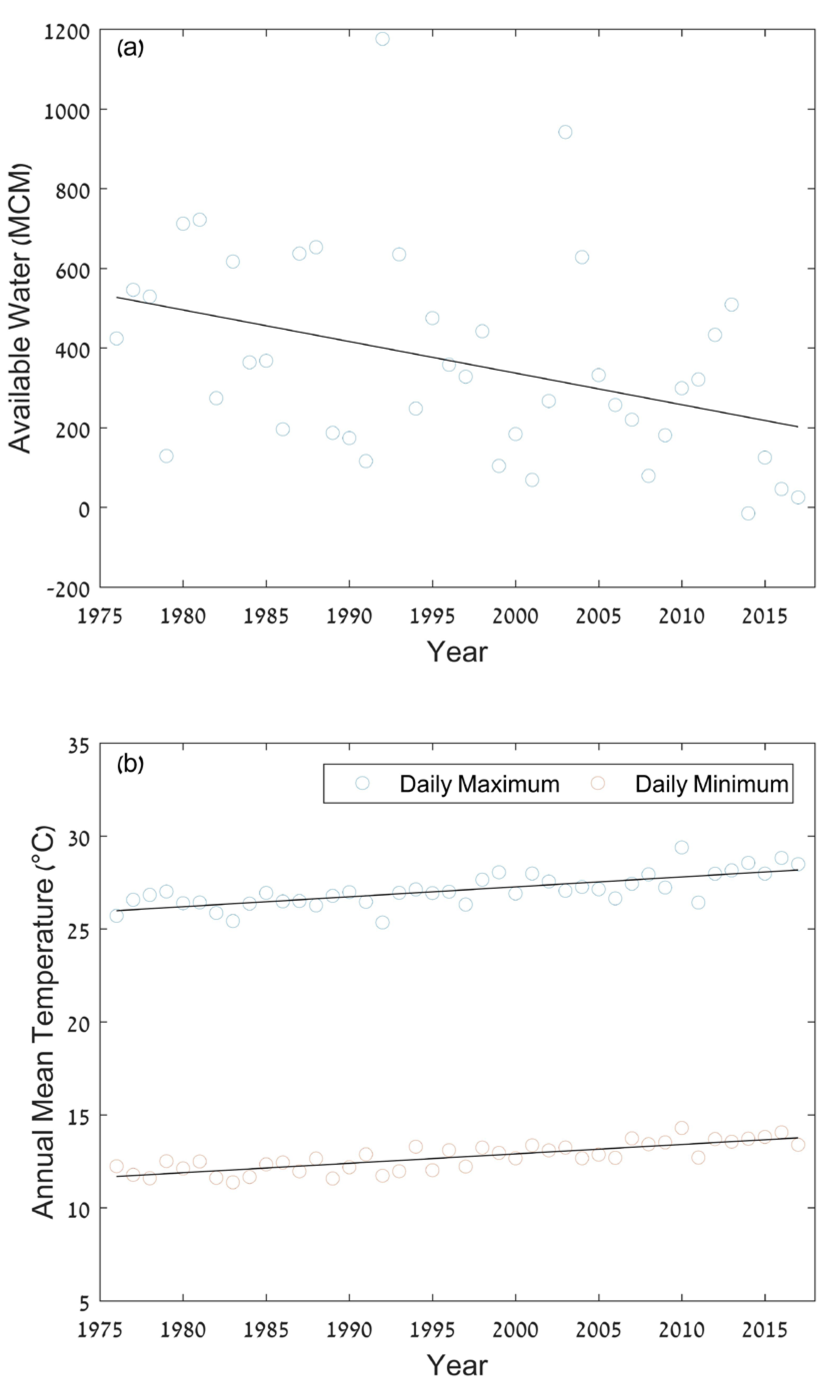
In Israel, the rainfall regimes in the last few decades reflect a consistent decreasing trend in average precipitation [14,15,16]. As Israel’s climate and hydrology patterns appear to be shifting toward dryer conditions with yet unfamiliar extent, we aim in this study to apply the Info-Gap Decision Theory to the Sea of Galilee (SoG) regional WSS, which is a significant part of the Israeli National Water System (INWS). Two weather-associated factors, rising temperatures and reduced rainfall, are the main drivers for the reduction in the SoG replenishment in recent years (see Section 2.2), where a 3.3% drop in rainfall per decade was observed during the last 40 years [14]. Thus, the SoG regional WSS management decisions will be investigated with IGDT in light of the uncertain behavior of future hydrological conditions by assessing the robustness of the system to various operation policies.

The remainder of this paper is organized as follows: Section 2 sets the background by briefly reviewing the available literature on IGDT applications for WSSs management problems under uncertainty, and gives an overview of the SoG WSS hydrological regime. Section 3 describes the concepts and structure of an Information Gap Decision Theory model. In Section 4, the formulation of the proposed regional WSS model is presented. The case study and the results are presented in Section 5. Finally, Section 6 concludes the study.

2. Background

2.1. Literature Review

In the past two decades, the Info-Gap decision theory gained a significant amount of applications in a variety of fields, such as engineering, economics, ecology, environmental protection, biology, medicine, project management, and national security [6,7]. However, among the multiple applications of IGDT, only a few were related to the domain of water resource systems, while only a handful addressed the planning and management of WSS problems, as we detail below.

Hipel and Ben-Haim [1] introduced IGDT to WSSs management problems by describing Info-Gap modeling to represent different sources of hydrological uncertainty. They illustrated decision making in watershed management problems using a few different Info-Gap models, each relevant to a different possible amount of prior information. They considered a lumped model of a WSS without modeling the spatial and temporal resolution of the problem (e.g., no conveyance network was considered). Woods et al. [11] used IGDT to assess the relative performance of various supply infrastructure portfolios meant to maintain the supply-demand balance in the Thames water resource system, UK. By comparing the robustness curves of the infrastructure options, they were able to prioritize the infrastructure options according to the projections of water availability, demand, and energy costs. A similar attempt to apply IGDT to quantitatively assess the robustness of various supply-side and demand-side management options was made by Korteling et al. [2] using a quasi-realistic water resources system based on a drift reservoir and demand node, located in southwest Cornwall, UK. In conjunction with IGDT, they included a Multi-Criteria Decision Analysis (MCDA) assessment for the management options to weight preferred performance results.

Matrosov et al. [9] demonstrated a joint application of Robust Decision Making (RDM) and IGDT frameworks to identify robust water supply portfolios for the planned capacity expansion of London’s water supply system in the Thames basin, UK. They showed that the methods are complementary since they provide different insights about the performance and vulnerabilities of the analyzed strategies. Matrosov et al. [9] concluded that a decision-maker would gain insights by deploying both frameworks in conjugation. Similar to Matrosov et al. [9], Roach et al. [3] compared the IGDT and Robust Optimization (RO) methods by assessing their applicability for a water resources management problem. They stressed that applying a wider range of decision methodologies will enable more encompassing investigation into potential future uncertainties.

In the broader context of water resources problems, IGDT was mainly applied to flood risk management problems. Hine and Hall [17] introduced IGDT to the field of flood management as an alternative to probability and fuzzy sets methods, to account for the uncertainty more adequately in highly uncertain fluvial rivers. They applied IGDT to a simple flood management problem to cost-effectively reduce the flood risk for surrounding residential properties. In their study, they evaluated the robustness of flood management decisions under uncertain upstream discharges into a floodplain. In a later work performed by Hine and Hall [5] for the river Trent catchment in the UK, an Info-Gap model was constructed around a parametric statistical flood discharges frequency analysis, resulting in a hybrid model of uncertainty. The robustness of a set of options for flood risk management accounted for two major sources of uncertainty: the flood depth model and the flow frequency. The analysis is considered a hybrid approach, in the sense that an Info-Gap model was used to analyze uncertainties in an underlying probabilistic model of the variability in fluvial flows. An additional application of Info-Gap analysis to a flood risk management problem was performed in [6], where few defense rising options have been considered to deal with potential damage caused by a given depth of floodwater. Therefore, the management decisions were related to the timing of interventions that should be taken. IGDT was tested as an alternative to probability and fuzzy sets theories while highlighting their unsuitability in cases of severe uncertainty.

In light of the above, there is a lack of studies that utilize the Info-Gap theory for the management of WSSs. The objective of this research is to develop a water management model based on the Info-Gap theory using optimization under uncertainty conditions to guide the long-term operation of the Sea of Galilee (SoG) WSS.

2.2. Sea of Galilee Hydrology and Climate Change Indications

The SoG watershed is divided between three Mediterranean countries, Israel, Lebanon, and Syria, and spans over 2730 km squared, where 25% of its area resides outside Israel’s borders [18]. It is situated in the northern part of Israel, which is, like other Middle East semi-arid regions, prone to dry conditions and limited water availability. The Sea of Galilee (Lake Kinneret) is the only natural surface freshwater reservoir in Israel and it is among the major water resources of the state [13,15]. The lake traditionally provided about a third of the country’s domestic, agricultural and industrial water requirements. Since the 1990s, extraction from Lake Kinneret exceeded the annual replenishment and its water levels declined to the lowest allowed level, endangering the ecological stability and the water quality of the lake [18]. In recent years, the Israeli government has undertaken extensive investments in water reclamation and desalination infrastructure in the country [14,15], while promoting water conservation. This has relieved the country’s reliance on the lake and significantly reduced the amount of water pumping. As a result, the lake’s ecological and environmental conditions have been improved, despite the persistent severe droughts in recent years [16]. Nowadays, the lake’s main uses are local water supply (mainly for agriculture), fishery, and tourism.

Climate change indicators are manifested in the SoG drainage basin. Using the Standard Precipitation Index (SPI), Givati et al. [19] indicated negative SPI (high level of aridity) of 11 and 17 during the 1927–1970 and 1970–2014 periods, respectively. This result indicates climate change as a higher level of aridity in the watershed. More specifically, the annual available water (inflows minus evaporation) in the SoG has decreased significantly during the last 40 years [14,15,16,19,20]. In Figure 1a, the linear regression line between the availability of SoG waters and Years (1976–2017) indicates a decline from 527 to 202 million cubic meters per year (MCM/Y). This result agrees with the conclusion of Gophen et al. [16] that indicated a decline from 470 to 225 MCM/Y in the period 1985–2016. Generally, there is a consensus among the Israeli government experts and researchers that climate change has an adverse effect on the SoG water level due to a combination of reduced precipitation and increased temperature/evaporation, which reduces the annual inflows. The flow in Israel’s streams and rivers is predominantly supplied by rainfall, where a general flow depletion trend has been measured across the SoG watershed over the past decade [16]. The extremeness of climate change in the watershed is highlighted when examining the Jordan River discharges during the last 40 years. Figure 3 in Gophen et al. [16] shows a decrease of about 53%. The increase in evaporation from the lake is associated with an increase in temperature in the watershed [16]. Figure 1b shows linear regressions between years and annual means of daily air maximum and minimum temperature measured in the KEFAR BLUM metrological station during 1976–2017. The annual maximum and minimum were elevated by about 2 °C during this period. This result agrees with Gophen et al. [16], which indicated increases of 2.7 °C and 1.5 °C in maximum and minimum temperature when analyzing data from DAFNA metrological station in the last 40 years.

These climate change indicators (Figure 1a,b) in the SoG watershed necessitate addressing severe uncertainty conditions in the planning and management of the SoG WSS. This is demonstrated by analyzing the recent years’ data and the SoG water level (Figure 1c), which shows five consecutive years of drought between years 2013–2018 [15]. The lake’s level reached −214.62 m in November 2018, which is defined as a black (catastrophic) line in the Israeli Water Authority (IWA). This drought was then followed by a wet winter (2019–2020) where the level of the lake increased by 5.73 m (a total volume increase of about 950 million cubic meters), leaving the lake almost full at level −208.89 m in May 2020. Although the water level of the lake did rise significantly, which ended the drought, the prospect for the coming future indicates that such extremism and high variability will challenge the water sector in the future [15,19]. Therefore, there are planned interventions in which desalination water will be “imported” from outside the SoG watershed to support the SoG WSS when needed.

The IWA employs a set of models for the planning and management of the regional WSS [13,21]. Although these models have been developed during the years to enable higher resolutions of various aspects of the system, support a multi-year time horizon, and account for both water quantity and quality, the models are essentially deterministic [21]. Attempts to account for uncertainty usually rely on a scenario-based approach to accommodate various possible realizations of the uncertain parameters. However, as explained previously, using deterministic models to make decisions under uncertainty might result in poor performance. Thus, in this study we present a decision support system based on the Info-Gap theory, which enables the decision-maker to come up with informed decisions by quantifying their confidence in the evaluated management policies through the evaluation of robustness to uncertainty [10,11]. By doing so, the Info-gap method allows the decision-maker to derive a trade-off between robustness and performance requirements. This trade-off enables the decision-maker to rank alternative policies based on their subjective attitude for balancing robustness and performance.

3. The Information Gap Decision Theory

A fundamental concept governing the IGDT approach is an expending uncertainty set relative to a nominal value (best estimate) of the uncertain parameter. When the uncertain parameter is equal to the nominal value, then no uncertainty is involved. Thus, as one step toward constructing the Info-Gap model, a nominal value needs to be obtained. A general representation of an optimization problem can be formulated as follows:

$$\begin{gathered} \widehat{f}=\underset{x}{\min }f\left(x,\theta \right) \\ subjectto \end{gathered}$$

(1)

$$h_i\left(x,\theta \right)\le 0\forall i=1‥m$$

(2)

$$x\ge 0$$

(3)

$$\theta \in U\left(\alpha \right)$$

(4)

where $x$ is the vector of decision variables, $\theta$ is the vector of uncertain parameters and $f\left(x,\theta \right)$ is the objective function. To achieve a feasible solution for the objective function, the constraints $h_i$ need to be fully satisfied. Note that we only include less-than-or-equal constraints because equality and larger-than constraints can be manipulated to be written as inequalities in a less-than-or-equal form.

When uncertainty is introduced, the uncertain parameter $\theta$ deviates from the nominal values $\widehat{\theta }$ by an unknown amount α. The behavior of the uncertain parameter is described by an uncertainty set $U\left(\alpha \right)$, which can be mathematically defined as follows:

$$U\left(\alpha \right)=\left\{\theta :\left|\theta -\widehat{\theta }\right|\le \sigma \alpha \right\}\alpha \ge 0$$

(5)

In Equation (5), the deviation is set relative to the standard deviation $\sigma$ of the uncertain parameters. That is, the expansion of the uncertainty set $U\left(\alpha \right)$ farther away from the nominal value $\widehat{\theta }$ is relative to the standard deviation.

Using Equations (1)–(4), we can determine the Base Run (BR) value of the objective function by setting the uncertain parameters $\theta =\widehat{\theta }$, that is, assuming there is no uncertainty involved:

$$\begin{gathered} {\widehat{f}}_{BR}= \underset{x}{\min }f\left(x,\widehat{\theta }\right) \\ subjectto \end{gathered}$$

(6)

$$h_i\left(x,\widehat{\theta }\right)\le 0\forall i=1‥m$$

(7)

$$x\ge 0$$

(8)

As Info-Gap analysis begins with the best estimate of the uncertain parameter, and solving Equations (6)–(8) will obtain the objective function value at that nominal value. This base run value (${\widehat{f}}_{BR})$ could be used as a reference to quantify the price-of-robustness.

Given a predefined $Budget$, we can search for the maximum allowed deviation α that can be tolerated, whilst still leading to performance within requirements. Therefore, the Info-Gap optimization problem is to find a decision variable $x$ which maximizes the allowed deviation α while still being feasible to all realizations in the uncertain set, as given in Equations (9)–(12).

$$\begin{gathered} \widehat{\alpha }= \underset{x}{\max }\alpha \\ subjectto \end{gathered}$$

(9)

$$\underset{\theta \in U\left(\alpha \right)}{\max }f\left(x,\theta \right)\le Budget$$

(10)

$$h_i\left(x,\theta \right)\le 0$$

(11)

$$x\ge 0$$

(12)

where $Budget$ represents the threshold for deviation from the BR value. When no uncertainty is involved, the total annual operating cost is equal to the base run value of the objective function, hence when $Budget={\widehat{f}}_{BR}$ we obtain the deterministic solution. When uncertainty is involved, increments of $Budget$ allow the decision-maker to explore different sizes of the uncertainty set by constructing a trade-off curve to represent the robustness of the system in different performance points. The robustness ($\widehat{\alpha }$) is the maximum allowed deviation α that still ensures the level of performance in which the operation cost is below $Budget$.

4. Formulation of the Proposed Regional WSS Model

This research presents an annual multi-year model for the management of water quantity allocation and storage management using optimization methods. We focus on the management of a regional WSS under hydrological uncertainty associated with the replenishment of natural resources. The objective that drives the decision is to minimize the present value of WSS operation cost, subject to physical, operational, and environmental constraints.

To apply the Info-Gap model, three elements are combined to assess the robustness to uncertainty: the system model, the uncertainty model, and the performance criteria [7]. As the drop in average annual precipitation is a major factor that is likely to influence the integrity of the SoG WSS, in this study we focus on the uncertainty in the surface water, represented as a vector $R^{tot}={[ R^{tot}{}_{t=1}, \cdots ,R^{tot}{}_{t=T_f}]}^T$, to investigate its influence on the system’s robustness. Under these settings, the robustness $\alpha$ is a measure of the maximum amount of uncertainty in the surface water that the system can tolerate while satisfying the constraint on the maximum budget (i.e., the performance criteria).

4.1. System Model—Physical and Operational Constraints

4.1.1. Water Conservation Law

The topology of the network is represented by the junction node connectivity matrix, where $A\in {ℝ}^{N_2\times M}$ has a row for each node and a column for each edge. The construction of matrix $A$ is demonstrated by a small hypothetical water supply system (Figure 2) that was used for model development and testing. The system is represented as a directed graph consisting of $N$ nodes connected by $M$ edges. The $M$ edges represent the links between nodes; links in which the direction of flow is not fixed can be represented by two edges, one in each direction. The nodes are composed of three subgroups: $N1$ are source nodes (e.g., desalination plant and reservoir) with one outgoing link from each source node; $N2$ are intermediate nodes, where two or more edges meet; and $N3$ are demand nodes, with one or more incoming links to each demand node.

The nonzero elements in each row are +1 and −1 for incoming and outgoing edges, respectively. The first two columns in A correspond to the links, which leave source nodes, while the last two columns correspond to the links ingoing demand nodes.

For each year t, the following system of linear equation ensures water conservation at the network nodes:

$$A{Q}_t=0\forall t$$

(13)

where $Q_t$ is the vector of discharges in the links (MCM/Y).

4.1.2. Limits on Water Quantities

The amount of water in all the system components (i.e., desalinated water from each plant, the discharges in the links, and extracted amount from the natural resources) is limited by an upper bound which represents maximum capacity, and by a lower bound (which may be zero or above) that represents operational constraints:

$$Q_t^{min} \le Q_t \le Q_t^{max}\forall t$$

(14)

4.1.3. Hydrological Water Balance in the Sources

The hydrological water mass balance ensures that the change in storage equals the difference between the total recharge and withdrawal over the operation horizon:

$$V_t= V_0+\left({\displaystyle \sum }_{i=1}^t{R}_i-P{\displaystyle \sum }_{i=1}^t{Q}_i\right) \forall t$$

(15)

where $V_t$ is a vector of the water volume (MCM) in the reservoirs at the end of year t; $V_0$ is a vector of the initial water volume (MCM) in the reservoirs; $P$ is a permutation matrix that extracts the outgoing flows of the reservoirs from the vector $Q_t$; and $R_t$ is a vector of the reservoirs recharge (MCM/Y). The recharge vector of the reservoirs is parametrized based on the total recharge in the watershed, $R_t^{tot}$, based on predetermined spatial distribution coefficients:

$$R_t={\beta }_s·R_t^{tot} \forall t$$

(16)

where ${\beta }_s$ is a vector of spatial distribution coefficients for water sources.

The water volume is bounded between a minimum and maximum water volume that represent physical conditions and/or operational constraints on the storage state:

$$V^{min} \le V_t \le V^{max}\forall t$$

(17)

It is noteworthy that some of the sources may not be capable of storing water (e.g., pumping directly from a river stream). In such cases, one can set $V^{min}= V^{max}=V_0=0$ to represent a direct inflow to the system without the ability to store water between years.

4.2. Objective Function

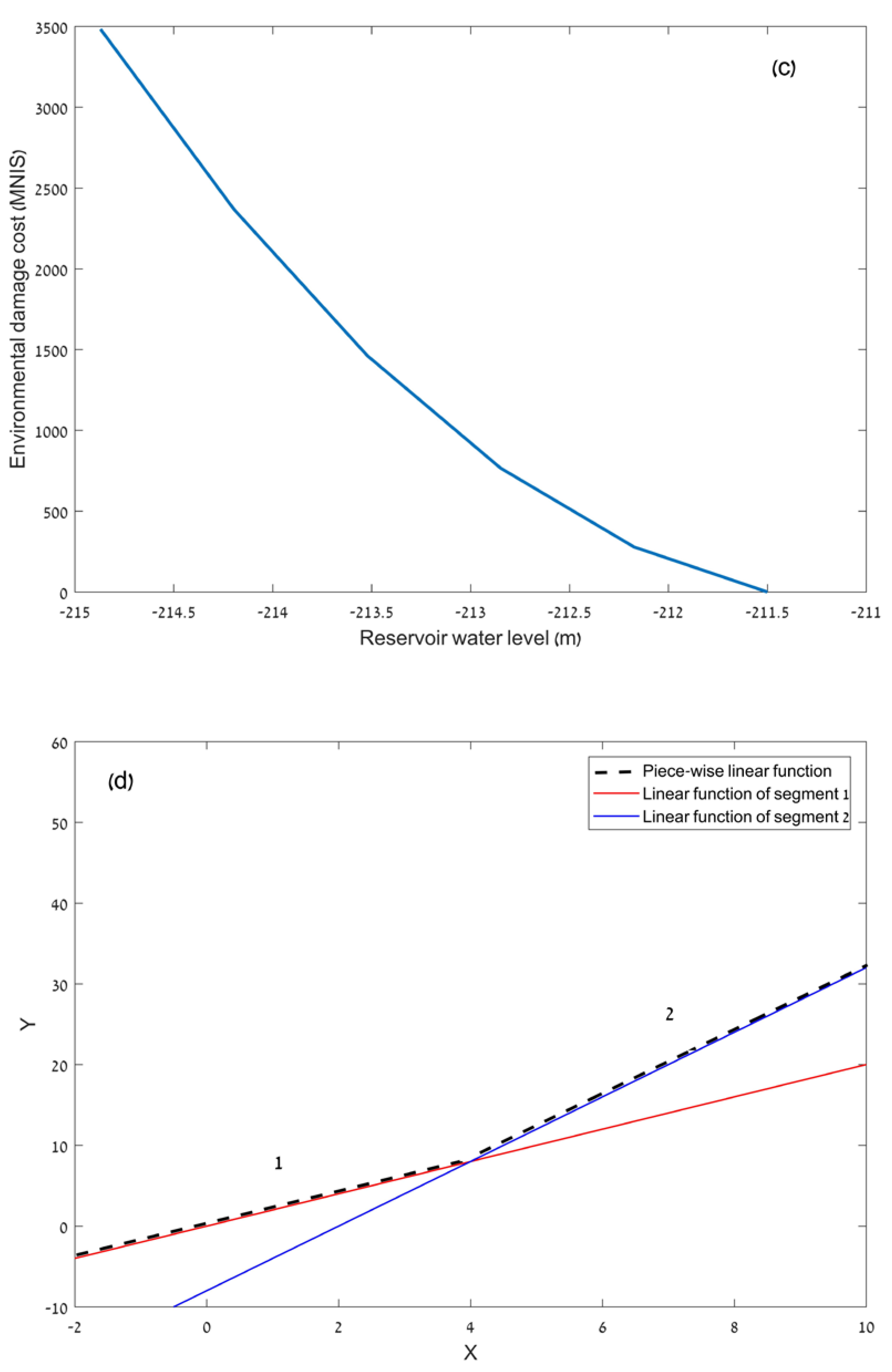
The objective is to operate the system with a minimum total cost composed of production cost, conveyance cost, and unsatisfied water demand cost (i.e., damage functions) over the operation horizon of $T_f$ years. These costs are modeled as nonlinear convex functions w.r.t the flows in the network. That is, at each link we have a cost function ${\varphi }_l\left(Q_t^l\right)$.

Additionally, we account for Environmental Cost $(EC$), which is a convex penalty function related to the final state of the water storage in the reservoirs ($V_{T_f}$) at the end of the operation horizon. This penalty represents the sustainability goal in which we require to return the reservoir storage to an adequate level at the end of the operation horizon. Henceforth, all values of water quantities ($Q_t$) are in Million Cubic Meters per year (MCM/Y) and the costs are in Million New Israeli Shekels (MNIS). The total cost, $TC$, is given as:

$$TC=\left\{{\displaystyle \sum }_{t=1}^{T_f}{\displaystyle \sum }_{l=1}^{nlinks}{\varphi }_l\left(Q_t^l\right)+EC\left(V_{T_f}\right)\right\}$$

(18)

For the sample network in Figure 2, an illustrative production/conveyance cost on link $Q_a$ is given in Figure 3a; an illustrative damage function on link $Q_{z1}$ is given in Figure 3b; and an illustrative Environmental Cost function is given in Figure 3c.

4.3. Deterministic LP Optimization Model

The cost functions, damage functions, and the environmental cost are represented in the model as nonlinear convex functions, thus leading to a nonlinear optimization problem. By approximating these nonlinear functions using convex piecewise-linear functions, the overall problem can be formulated as a Linear Programming (LP) model which could be efficiently solved by available optimization solvers (in this study we used LINPROG solver available within the MATLAB optimization toolbox).

Piecewise linearization is performed by dividing the nonlinear convex functions into linear segments, then, owing to the convexity, the value of the piecewise function could be obtained by applying the maximum operator overall segments. Thus, for a given convex function $\varphi \left(Q\right)$, an approximated convex piecewise-linear function $\widehat{\varphi }\left(Q\right)$ could be formulated as follows:

$${\varphi }_l\left(Q_t^l\right)\approx {\widehat{\varphi }}_l\left(Q_t^l\right)=\underset{i=1\dots m_l}{\max }(a_i^l·Q_t^l+b_i^l) \forall \mathrm{l}\hspace{1em}\forall \mathrm{t}$$

(19)

where $m_l$ is the number of linear segments in link $l$ and $a_i^l,b_i^l$ are the coefficient of the linear segments. Figure 3d shows a convex piecewise-linear function with two segments. The figure shows that the linear function of the first segment obtains the maximum values in the range of the first segment (i.e., −2:4), while the linear function of the second segment obtains the maximum values in the range of the second segment (i.e., 4:10). Thus, we can write the piece-wise linear function in terms of a maximum operator as shown in Equation (19). The maximum operator in Equation (19) could then be formulated as an LP by introducing an auxiliary scalar variable ${\phi }_t^l$, which represents the value of the piece-wise linear function. The equivalent LP can be formulated as:

$$\begin{gathered} min {\mathsf{\phi }}_{\mathrm{t}}^{\mathrm{l}} \\ subjectto \end{gathered}$$

(20)

$${\mathrm{a}}_{\mathrm{i}}^{\mathrm{l}}·{\mathrm{Q}}_{\mathrm{t}}^{\mathrm{l}}+{\mathrm{b}}_{\mathrm{i}}^{\mathrm{l}}\le {\mathsf{\phi }}_{\mathrm{t}}^{\mathrm{l}}$$

(21)

Applying convex piecewise-linear approximation to all the cost functions guarantees that the objective function and the constraints will be formulated as an LP. The overall deterministic (i.e., assuming $R_t^{tot}$ is known) is given as:

$$\begin{gathered} \min \left\{{\displaystyle \sum }_{\mathrm{t}=1}^{{\mathrm{T}}_{\mathrm{f}}}{\displaystyle \sum }_{\mathrm{l}=1}^{\mathrm{nlinks}}{\mathsf{\phi }}_{\mathrm{t}}^{\mathrm{l}}+{\mathsf{\phi }}^{\mathrm{EC}}\right\} \\ subjectto \end{gathered}$$

(22)

$${\mathrm{AQ}}_{\mathrm{t}}=0 \forall \mathrm{t}$$

(23)

$${\mathrm{V}}_{\mathrm{t}}={\mathrm{V}}_0+\left({\displaystyle \sum }_{\mathrm{i}=1}^{\mathrm{t}}{\mathsf{\beta }}_{\mathrm{s}}·{\mathrm{R}}_{\mathrm{t}}^{\mathrm{tot}}-\mathrm{P}{\displaystyle \sum }_{\mathrm{i}=1}^{\mathrm{t}}{\mathrm{Q}}_{\mathrm{i}}\right)\forall \mathrm{t}$$

(24)

$${\mathrm{a}}_{\mathrm{i}}^{\mathrm{l}}·{\mathrm{Q}}_{\mathrm{t}}^{\mathrm{l}}+{\mathrm{b}}_{\mathrm{i}}^{\mathrm{l}}\le {\mathsf{\phi }}_{\mathrm{t}}^{\mathrm{l}} \forall \mathrm{t} \forall \mathrm{l} \forall \mathrm{i}=1\dots {\mathrm{m}}_{\mathrm{l}}$$

(25)

$${\mathrm{a}}_{\mathrm{i}}^{\mathrm{EC}}·{\mathrm{V}}_{{\mathrm{T}}_{\mathrm{f}}}+{\mathrm{b}}_{\mathrm{i}}^{\mathrm{EC}}\le {\mathsf{\phi }}^{\mathrm{EC}}\forall \mathrm{i}=1\dots {\mathrm{m}}_{\mathrm{EC}}$$

(26)

$${\mathrm{Q}}_{\mathrm{t}}^{\min }\le {\mathrm{Q}}_{\mathrm{t}}\le {\mathrm{Q}}_{\mathrm{t}}^{\max } \forall \mathrm{t}$$

(27)

$${\mathrm{V}}^{\min } \le { \mathrm{V}}_{\mathrm{t}} \le { \mathrm{V}}^{\max } \forall \mathrm{t}$$

(28)

The formulation above is a deterministic formulation in which the recharge is an assumed known parameter. In the next section, we show the Info-Gap formulation of the optimization problem above.

4.4. Info-Gap Model

As explained previously, to apply the Info-Gap model, three elements are combined to assess the robustness to uncertainty: the system model, the uncertainty model, and the performance criteria [7]. The system model and the performance criteria (budget) were presented in the previous section. In the following section, we describe the uncertainty model formulation.

For the uncertainty Info-Gap model, there is a wide range of commonly used Info-Gap models. The formulation and choice of an uncertainty model depend on the type and the quantity of available information [1,10]. In our case, the total available surface water ($R_t^{tot}$) is considered uncertain and may vary largely among the years of the operation horizon. Therefore, the deviation $\alpha$ from the nominal value ${\widehat{R}}_t^{tot}$ is measured relative to the standard deviation (${\sigma }_R$). As such, we consider a fractional-error Info-Gap model [8,9]:

$$U\left(\alpha \right)=\left\{R_t^{tot} : R_t^{tot}\ge 0,\left|\frac{R_t^{tot}-{\widehat{R}}_t^{tot}}{{\sigma }_R} \right|\le \alpha \forall t\right\} \alpha \ge 0$$

(29)

This model creates an expending interval around the nominal value ${\widehat{R}}_t^{tot}$:

$$U\left(\alpha \right)=\left\{R_t^{tot} :\max \left[0,{\widehat{R}}_t^{tot}-\alpha \times {\sigma }_R\right]\le R_t^{tot}\le {\widehat{R}}_t^{tot}+\alpha \times {\sigma }_R \forall t\right\}\mathsf{\alpha }\ge 0$$

(30)

where $U\left(\alpha \right)$ is a nested subset around a point estimate ${\widehat{R}}_t^{tot}$, thus $R_t^{tot}$ deviates from the nominal value by an unknown amount of uncertainty $\alpha$. The family of nested subsets (Figure 4) is bounding the variation of the recharge around the nominal value. The greater the value of $\alpha$, the greater the possibilities of $R_t^{tot}$. However, in our case, the amount of available surface water must have a non-negative value. This implies that:

$$0\le \mathsf{\alpha }\le \frac{{\widehat{R}}^{\mathrm{tot}}}{{\mathsf{\sigma }}_{\mathrm{R}}}$$

(31)

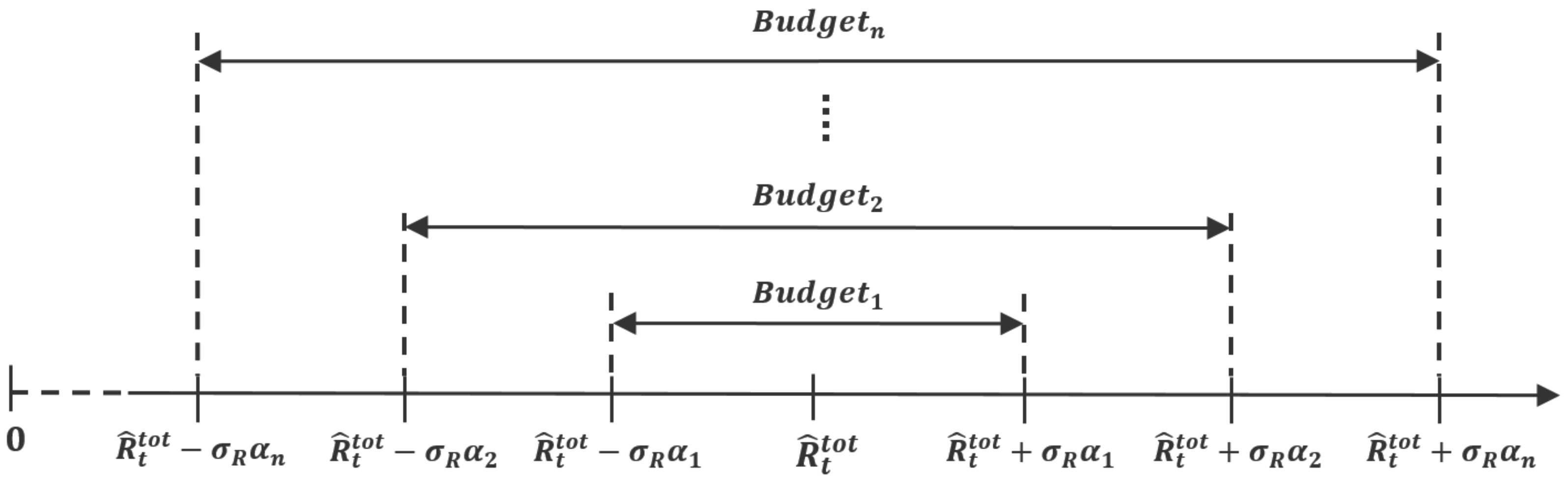
This work uses the average annual operation budget as a performance criterion of the system. Namely, the budget is used in the Info-Gap framework as a threshold to define the maximum achievable robustness. Figure 4 shows that the larger the budget, the larger the deviation that can be tolerated. More specifically, $Budge{t}_n>Budge{t}_2>Budge{t}_1$ lead to robustness (i.e., allowed deviation within budget) ${\alpha }_n>{\alpha }_2>{\alpha }_1$.

The Info-Gap framework seeks the maximum robustness for a specified budget, thus the optimization problem can be formulated as detailed in Equations (32)–(34) below. For ease of notation, the decision variables $Q_{t },V_t , {\phi }_t^l , {\phi }^{EC}$ are collected in a decision vector $x$ and the set of constraints in Equations (23)–(28) is defined as a set $X$. Note that the set of constraints depends on $R^{tot}$ because of the constraint in Equation (24). That is, a feasible decision vector should be $x\in X\left(R^{tot}\right)$.

$$\begin{gathered} \max \mathsf{\alpha } \\ subjectto \end{gathered}$$

(32)

$$\left(\underset{ {\mathrm{R}}^{\mathrm{tot}}\in \mathrm{U}\left(\mathsf{\alpha }\right)}{\max }\underset{ \mathrm{x} \in \mathrm{X}\left({\mathrm{R}}^{\mathrm{tot}}\right)}{\min }{\displaystyle \sum }_{\mathrm{t}=1}^{{\mathrm{T}}_{\mathrm{f}}}{\displaystyle \sum }_{\mathrm{l}=1}^{\mathrm{nlinks}}{\mathsf{\phi }}_{\mathrm{t}}^{\mathrm{l}}+{\mathsf{\phi }}^{\mathrm{EC}}\right)\le \mathrm{Budget}$$

(33)

$$0\le \mathsf{\alpha }\le \frac{{\widehat{\mathrm{R}}}^{\mathrm{tot}}}{{\mathsf{\sigma }}_{\mathrm{R}}}$$

(34)

The first constraint in the optimization problem above implies that the worst optimum solution of the cost inside the uncertainty set should be less than $Budget$. This means that the system cost will be guaranteed to yield a cost less than $Budget$ for any realization $R^{tot}$ inside the uncertainty set. Chinneck and Ramadan [22] study the worst optimum solution of linear programs with interval uncertainty sets. In Theorem 6 of their work, they prove that the worst optimum solution will be obtained on an extreme scenario of the interval uncertainty sets. In our context, it is either $R^{tot}={\widehat{R}}^{tot}-{\sigma }_R\alpha$ or $R^{tot}={\widehat{R}}^{tot}+{\sigma }_R\alpha$. Since the optimization model in Section 4.3 focuses on water shortages costs (e.g., damage cost for unsatisfied demand, environmental cost of low water levels), the relevant extreme scenario for our problem is $R^{tot}={\widehat{R}}^{tot}-{\sigma }_R\alpha$. In light of the above, the optimization problem in Equations (32)–(34) could be written as the following LP:

$$\begin{gathered} \underset{\mathrm{x},\mathsf{\alpha }}{\max }\mathsf{\alpha } \\ subjectto \end{gathered}$$

(35)

$${\displaystyle \sum }_{\mathrm{t}=1}^{{\mathrm{T}}_{\mathrm{f}}}{\displaystyle \sum }_{\mathrm{l}=1}^{\mathrm{nlinks}}{\mathsf{\phi }}_{\mathrm{t}}^{\mathrm{l}}+{\mathsf{\phi }}^{\mathrm{EC}}\le \mathrm{Budget}$$

(36)

$${\mathrm{AQ}}_{\mathrm{t}}=0\forall \mathrm{t}$$

(37)

$${\mathrm{V}}_{\mathrm{t}}={\mathrm{V}}_0+\left({\displaystyle \sum }_{\mathrm{i}=1}^{\mathrm{t}}{\mathsf{\beta }}_{\mathrm{s}}·\left({\widehat{\mathrm{R}}}^{\mathrm{tot}}-{\sigma }_R\alpha \right)-\mathrm{P}{\displaystyle \sum }_{\mathrm{i}=1}^{\mathrm{t}}{\mathrm{Q}}_{\mathrm{i}}\right)\forall \mathrm{t}$$

(38)

$${\mathrm{a}}_{\mathrm{i}}^{\mathrm{l}}·{\mathrm{Q}}_{\mathrm{t}}^{\mathrm{l}}+{\mathrm{b}}_{\mathrm{i}}^{\mathrm{l}}\le {\mathsf{\phi }}_{\mathrm{t}}^{\mathrm{l}} \forall \mathrm{t} \forall \mathrm{l} \forall \mathrm{i}=1\dots {\mathrm{m}}_{\mathrm{l}}$$

(39)

$${\mathrm{a}}_{\mathrm{i}}^{\mathrm{EC}}·{\mathrm{V}}_{{\mathrm{T}}_{\mathrm{f}}}+{\mathrm{b}}_{\mathrm{i}}^{\mathrm{EC}}\le {\mathsf{\phi }}^{\mathrm{EC}} \forall \mathrm{i}=1\dots {\mathrm{m}}_{\mathrm{EC}}$$

(40)

$${\mathrm{Q}}_{\mathrm{t}}^{\min }\le {\mathrm{Q}}_{\mathrm{t}}\le {\mathrm{Q}}_{\mathrm{t}}^{\max }\forall \mathrm{t}$$

(41)

$${\mathrm{V}}^{\min }\le {\mathrm{V}}_{\mathrm{t}}\le {\mathrm{V}}^{\max }\forall \mathrm{t}$$

(42)

$$0\le \mathsf{\alpha }\le \frac{{\widehat{\mathrm{R}}}^{\mathrm{tot}}}{{\mathsf{\sigma }}_{\mathrm{R}}}$$

(43)

5. Case Study

In this section, the Info-Gap model described in Section 4.4 is applied to the optimal multi-year management of the SoG WSS. The water system layout is shown in Figure 5. It has one reservoir (Sea of Galilee), 9 surface sources, 7 ground water sources, 3 water imports (representing water transfer from national water supply system), 16 demand zones, and 59 links.

In the current study, we consider the hydrological uncertainty of the surface water in the watershed. The total surface water is considered uncertain according to the uncertainty set defined in Equation (29). The surface water is distributed between nine surface water sources according to predetermined spatial distribution coefficients, which are obtained based on the analysis of historical records. Thus, the surface water capacity is uncertain, while the other sources (i.e., ground water production and import) are deterministic and can produce any amount between pre-specified bounds. In terms of cost, the surface water is free, the ground water costs range between 0 and 1 NIS per ${\mathrm{m}}^3$, while the water import costs range between 1.5 and 2.5 NIS per ${\mathrm{m}}^3$. As such, import sources can produce a large and reliable amount of water, but at a greater cost. This operational trade-off between the deterministic-expensive vs. uncertain-free sources will be examined in the results.

For the next 3 years, we consider 30 equally likely hydrological scenarios of the total surface water in the watershed, as shown in Figure 6. These forecasts aim to emulate different possible future scenarios, ranging from low precipitation series to high precipitation series. The nominal scenario (i.e., the scenario with average total inflow) is highlighted in green in Figure 6. This nominal scenario is used to construct the uncertainty set of the Info-Gap model as detailed in Equation (29), where ${\sigma }_R=150$ MCM.

The development and implementation of the mathematical model were programmed using MATLAB and the YALMIP toolbox [23]. YALMIP is used to model and solve the optimization model by interfacing external solvers via simple mathematical programming syntax. In this study, the optimization problem was solved using the LP solver, LINPROG, which is provided within the optimization toolbox of MATLAB.

5.1. Operation Policies

An important aspect of solving uncertain models is the sequence in which decisions alternate with uncertain observations [4]. That is, which decisions should be taken before uncertainty is revealed and which decisions are recourse decisions that adapt to the revealed uncertainty. In our context, we must distinguish between the operation policy that the decision-maker determines before uncertainty is revealed and recourse decisions that adapt to the revealed uncertainty. For example, if we consider one demand zone $\left(DZ\right)$ which is fed by one ground water source $\left(GW\right)$ and one uncertain surface water source $\left(SW\right)$ (Figure 7), we cannot set both $Q_{GW}$ and $Q_{DZ}$ since the problem will be infeasible for all realizations of the uncertain source, except $R=Q_{DZ}-Q_{GW}$. A better modeling approach is to set one of the decisions (e.g., $Q_{GW}$) as an operation policy that should be determined by the decision-maker before uncertainty is revealed, and the other one (e.g., $Q_{DZ}$) as a recourse decision that takes value depending on the observed $R$ and the determined operation policy (i.e., $Q_{DZ}=R+Q_{GW}$).

The operation policy represents the immediate commitment of the decision-maker that should be made in face of the uncertain future, while the recourse decisions are decisions that represent the reaction of the system to the revealed future scenario. In our case study, the WSS operation is solved for three years operation horizon, where the operation policy that represents the immediate commitment of the decision-maker is comprised of the ground water productions (seven decision variables) and the water imports (three decision variables) in the first year. In total, an operation policy is comprised of determining 10 decision variables in the first year of the operation horizon. These 10 variables could be determined using deterministic optimization or optimization under uncertainty methods. In this study, we examine three operational policies and show their robustness based on the Info-Gap framework.

First, we consider the Nominal Policy (NP), which is obtained by solving a deterministic optimization problem with the nominal scenario highlighted in Figure 6. In the NP, the decision-maker assumes that the nominal scenario will be realized and commits to ground water production and water import during the first year according to this assumption. Second, we consider the Scenario Based Policy (SBP), in which the decision-maker accounts for all 30 forecast scenarios in Figure 6. In this case, as the scenarios are equally likely, the decision-maker solves each of the scenarios and then commits to ground water production and water import during the first year based on the average amounts obtained from the solutions of the 30 scenarios. Third, we consider the Robust Policy (RP), which is obtained by solving the Info-Gap model Equations (35)–(43) with a budget of 400 MNIS that guarantees the robustness of 1.5, as will be explained in the next section. Figure 8 shows the obtained operation policies (i.e., ground water productions and water imports in the first year) using the three approaches discussed above.

As shown in Figure 8, the NP relies on ground water only, without the need to utilize expensive imported water. That is, if the nominal scenario is realized, the system can rely on local sources without the need for water transfer from the national water system. The SBP shows more ground water withdrawal as well as the utilization of water imports. This is because some of the scenarios considered (see Figure 6) are dry scenarios that require more ground water withdrawal and transferring water from the national water system. The different utilization of the sources (e.g., high amount in $I{m}_2$ compared to $I{m}_1$ and $I{m}_3$) is attributed to the different production and conveyance costs in the system. The RP exhibits the largest utilization of all ground water sources and water imports. This is because the RP, which is designed to guarantee a robustness of 1.5, accounts for a dry scenario that deviates from the nominal scenario by as high as $1.5\times {\sigma }_R=225$ MCM.

5.2. Operational Policies Comparison

The robustness of the three operation policies discussed in the previous section is analyzed using the Info-Gap framework. The Info-Gap formulation in Equations (35)–(43) is applied using a two-stage recourse approach, where the operation policies are implemented at the beginning of the operation horizon before the uncertainty is revealed, and the other decisions are recourse decisions that are determined within the Info-Gap formulation. More specifically, each of the operation policies will impose equality constraints on the Info-Gap formulation by setting the 10 decision variables of the operation policy to the values shown in Figure 8. For example, to evaluate the robustness of the NP, the Info-Gap formulation in Equations (35)–(43) is solved with additional constraints that set the first-year ground water productions and water imports to the values shown in red in Figure 8.

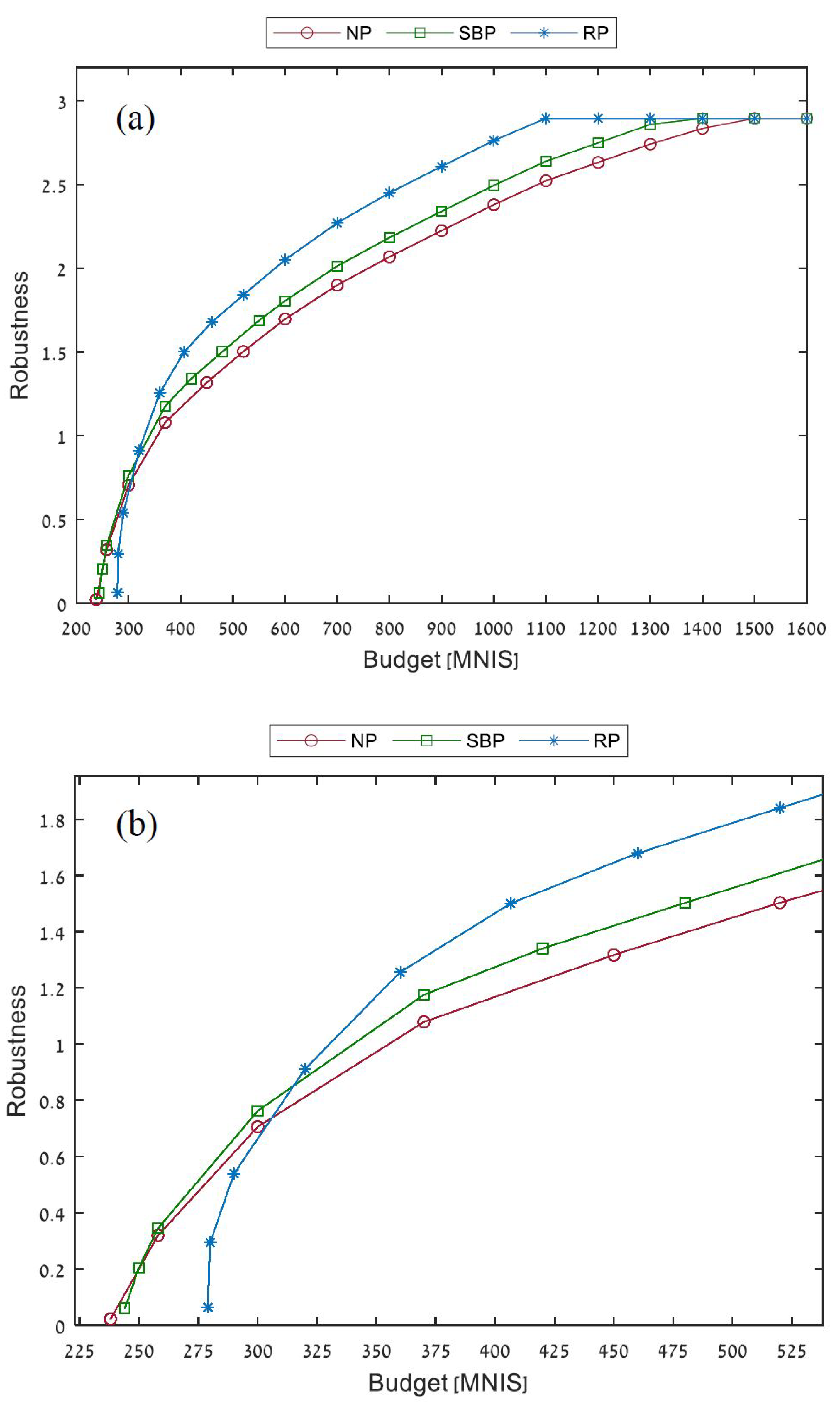
Figure 9a,b shows the trade-off between robustness and annual budget for each of the three operation policies. These trade-offs are obtained by solving the Info-Gap formulation in Equations (35)–(43) for increasing series of annual budgets for each of the three operation policies. For each point in the robustness trade-off, we have the decision vector corresponding to that point. Namely, for any given budget the optimization problem provides the optimal decisions for the entire three years operation horizon that maximize the robustness of the system operation under the operation policy constraints.

For example, the trade-off of the NP shows robustness vs. budget in case the decision-maker relies on the nominal scenario to dictate the productions and water import in the first year. The different points on the trade-off show the maximum deviations (in standard deviations units) from the nominal surface water amount, which can be tolerated under different budgets. For example, if the NP is implemented and the annual budget is 238 MNIS, then the robustness is zero. This indicates that we cannot tolerate any uncertainty with a budget of 238 MNIS under the NP, while to tolerate a deviation of $1.5\times {\sigma }_R=225$ MCM in the NP, an annual budget of 520 MNIS is required. The results also show that the NP can reach a maximum robustness of 2.895 (i.e., tolerate a deviation of $2.895\times {\sigma }_R=434.25$ MCM) with an annual budget of 1500 MNIS.

Comparing the different trade-offs from the three operation policies shows that the RP is superior for budgets larger than 307 MNIS. This is demonstrated by higher robustness for the given budget obtained by the RP. For instance, when the budget is 800 MNIS the RP can reach a robustness of 2.451, while the SBP and the NP can only reach a robustness of 2.183 and 2.068, respectively. Another way to interpret the results is that the RP can tolerate a deviation of $1.5\times {\sigma }_R=225$ MCM while guaranteeing a budget below 400 MNIS, while the SBP and NP will require budgets of 480 MNIS and 520 MNIS, respectively, to tolerate the same deviation.

The maximum robustness in all operation policies is 2.895. However, the RP reaches this robustness with a smaller budget of 1100 MNIS as opposed to 1400 MNIS and 1500 MNIS in the SBP and NP, respectively. To conclude, the results show that for a budget larger than 307 MNIS, the RP can cope better with uncertainty by maximizing the uncertainty horizon that can be tolerated for a given budget. Comparing the SBP with the NP shows that the SBP can tolerate larger uncertainty. This is because the SBP operation policy is derived from 30 scenarios that include dry scenarios, which result in a more robust operation policy compared to the NP.

Figure 9b shows the trade-off for low budgets. The results show that for a low budget (budget < 307 MNIS), the RP has less robustness, that is, it can tolerate less uncertainty compared to the SBP and NP. In other words, more budget is required to tolerate a small level of uncertainty in the RP. For example, to tolerate a deviation of $0.4\times {\sigma }_R$, the SBP and the NP can guarantee a budget below 262 MNIS and 268 MNIS, respectively, whilst the RP will have a higher budget of 285 MNIS. This result can be explained by the fact that RP is a worst-case oriented policy that is expected to perform optimally in extreme scenarios, while SBP and NP are expectation-oriented policies that are expected to perform optimally around the nominal scenarios. Nonetheless, for a robustness of 0.4, the additional budget in the RP compared to the NP is only 17 MNIS, while for a high robustness of 1.5 the NP will have a high additional budget of 100 MNIS compared to the RP. As such, for risk aversion, the decision-maker may prefer the RP, which behaves optimally in extreme scenarios.

5.3. Examining the Operation Policies under Monte-Carlo Simulations

For water resources management models, we are often able to generate a large number of scenarios that form an approximation of the underlying random process. These sets of scenarios may be obtained by simulation using stochastic models, historical data, and expert forecasting for extreme scenarios. One of the most common ways of generating individual scenarios is Monte-Carlo Sampling [2]. Using this approach, random variables are generated from their known (or assumed) distribution, thus replacing continuous probability space with a finite space consisting of the samples. The generated samples are then used to simulate the possible future values of the uncertain variables [5].

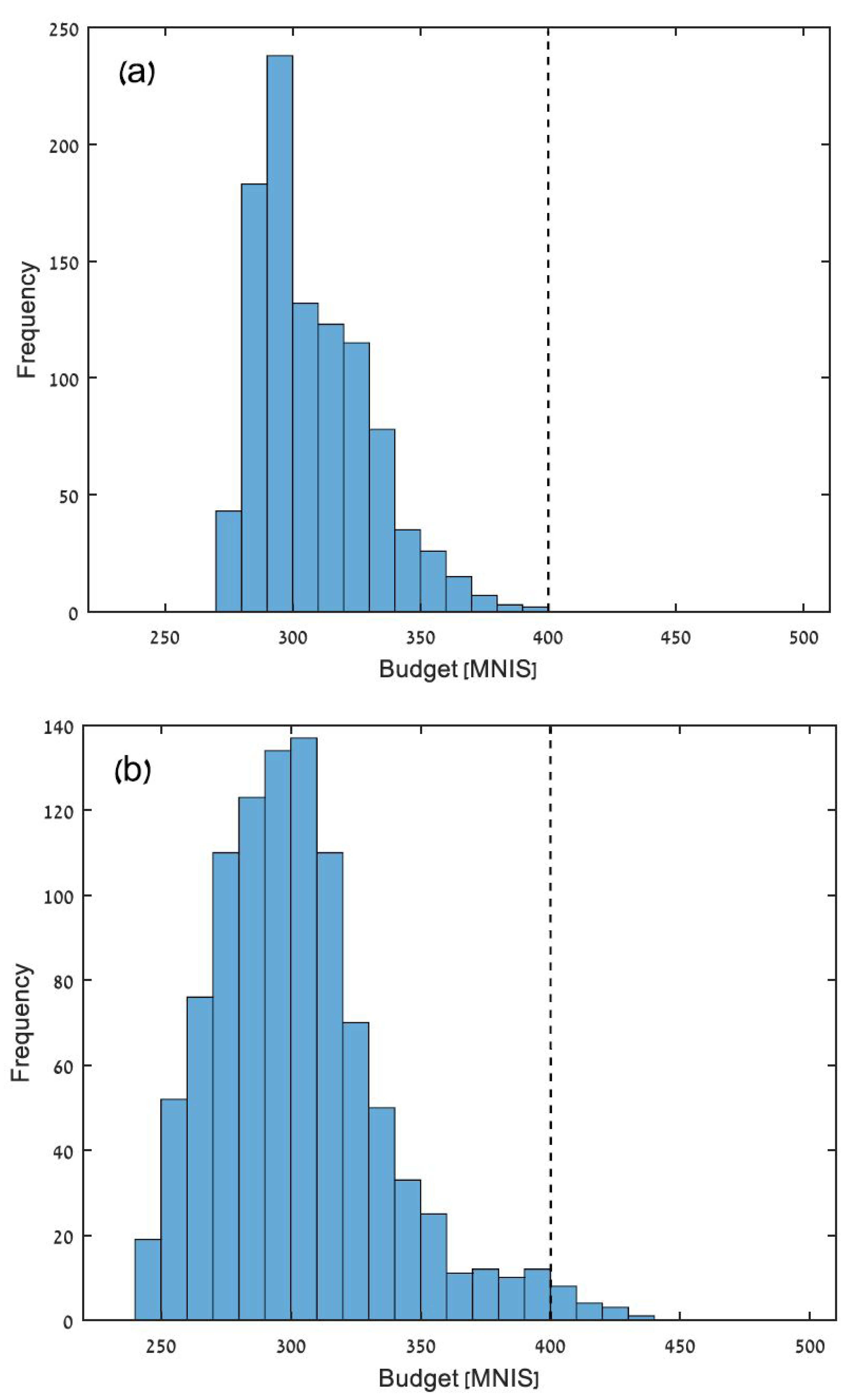
We would like to emphasize that the IGDT does not require Monte-Carlo simulation or any other probabilistic assumptions. In this section, we only use Monte-Carlo simulations to evaluate the different operation policies and compare the results to the budget guarantee provided by the IGDT. As indicated previously, in our case study we focus on dry scenarios and the resulting water shortages. Thus, we have generated 1000 uniformly random samples between $R_t^{tot}-1.5\times {\sigma }_R$ and ${\widehat{R}}_t^{tot}$ for the three years operation horizon. The SoG WSS model is solved for each of the 1000 samples under the three operation policies to obtain the budget histograms, as shown in Figure 10.

The results obtained by the Monte-Carlo simulations (Figure 10) show that the RP guarantees a budget below 400 MNIS for deviation up to $1.5\times {\sigma }_R$. This budget guarantee agrees with the IGDT analysis shown in Figure 9b for a robustness level of 1.5.

As discussed in the previous section, the NP and SBP are less robust compared to the RP under extreme scenarios. As such, both of these policies exceed the 400 MNIS budget guarantee of the RP, as shown in Figure 10b,c. That is, both require a budget greater than 400 MNIS to cope with a deviation of $1.5\times {\sigma }_R$. The budget violation in the NP and SBP relative to the RP budget guarantee is 25% and 10%, respectively. On the other hand, the average budgets in the histograms are 314, 303, and 308 for the NP, the SBP, and the RP, respectively, showing that the SBP performs better on average when compared to the RP. Nonetheless, the deviation in the average budget is (308 − 303)/303 = 1.7% compared to a budget guarantee reduction of (440 − 400)/400 = 10% for extreme scenarios. The empirical results obtained from the Monte-Carlo simulations analysis fortify the advantages of the RP. It is noteworthy that investigating the system robustness via the IGDT is more computationally efficient, since the budget required for each robustness value is obtained through the trade-off curve (e.g., Figure 9a) without the need to empirically rely on thousands of random simulations and assumptions on the probabilistic distribution of the random data.

5.4. Sensitivity Analysis

The IGDT robustness evaluation can also facilitate sensitivity analysis for important parameters in the model. For example, an important parameter in the SoG WSS is the minimum flow in link L30, which represents the minimum flow needed for recreational purposes and the natural conservation of the Upper Jordan River. In recent years, the annual average flow of the Upper Jordan River has dropped to roughly half of the annual average flow, which was typically over 100 MCM [24].

To examine the impact of minimum flow regulation, a sensitivity analysis was performed by running the Info-Gap model for different levels of $Q_{l_{30}}^{min}$. Requiring minimum flow in link L30 implies that less surface water should be used in the upper part of the system in order to meet the minimum flow constraint. As such, the system is forced to rely on more expensive imported water and increased ground water production. This increases the operation cost, which leaves less budget to tolerate the uncertainty (i.e., reduced robustness).

Figure 11 shows the robustness vs. budget trade-off of the RP for different levels of minimum flow regulation in link L30. The comparison of the obtained trade-offs shows that the robustness vs. budget trade-off shrinks when the minimum flow regulation is stricter (i.e., $Q_{l_{30}}^{min}$ is higher). For example, the RP can tolerate a deviation of $2.895\times {\sigma }_R=434.25$ MCM with a budget of 1100 MNIS when there is no minimum flow requirement, but it can only tolerate a deviation of $1.463\times {\sigma }_R=219.45$ MCM for the same budget when a minimum flow regulation of 200 MCM is imposed on link L30. An important aspect of the results shown in Figure 11 is the overlapping trade-offs in the budget range of 279–350 MCM, which indicates that the minimum flow regulation in link L30 has little impact on the robustness within this budget range. Another important observation is that the length of the flat segments in the curves is increasing for increased minimum flow regulation in link L30. This indicates that for higher minimum flow regulation, the budget has less impact on the trade-off (i.e., the robustness is fixed regardless of the budget amount). In other words, the budget becomes a non-limiting factor in determining the robustness as the minimum flow requirement increases (i.e., other factors such as conveyance and production capacities become limiting factors).

We emphasize that the above is just a demonstration of how the IGDT could be used for sensitivity analysis. Many other sensitivity analyses might be performed to explore the impact on the system robustness. Future studies may use the IGDT for sensitivity analysis to explore other impacts on the system robustness, such as topological changes (e.g., adding new links or exploring planning alternatives).

6. Discussion and Conclusions

In this study, we developed a water management model based on the IGDT to investigate climate change impacts on WSS management decisions. We focused on the impact of climate change related to hydrological uncertainty, where only the replenishment into the natural resources is taken as an uncertain parameter. To incorporate explicit considerations of uncertainty, an appropriate decision-making framework under uncertainty should be selected such that the real nature of the problem will be reflected during the modeling process, and that the results are usable in the real world. The tools required to support decision making in the face of uncertainty must be flexible enough to allow the testing of trade-offs between various characteristics of future outcomes, efficient enough to run quickly for different inputs (i.e., computational efficiency), and transparent enough to convey to the decision-makers the full range of consequences of different possible decisions. We demonstrated the IGDT as a tool that preserves the properties above for the multi-year SoG WSS management problem.

Our results demonstrate the importance of introducing uncertainty into deterministic models when evaluating climate change impacts, as the solution can change dramatically when recharge uncertainty is considered. In cases of highly uncertain future conditions, the uncertainty could be represented in the Info-Gap model using the concept of uncertainty sets. We considered the sequence in which decisions alternate with observations and showed that in cases where all decisions are taken before the uncertainty is revealed, the problem may become infeasible for most of the realizations of the uncertain source. Thus, for policy selection, we implemented a two-stage recourse framework. In the first stage, some decisions (i.e., an operation policy) are implemented at the beginning of the operation horizon before the uncertainty is revealed, and this represents the immediate commitment made, while in the second stage recourse decisions are allowed to adapt to the revealed uncertainty.

The Info-Gap model enables the decision-maker to examine the trade-off between the amounts of robustness gained for every budget limit. That is, for predetermined operation policies, the performance of each policy is examined by searching for the robust optimal decision at each budget limit. In this study, we examined three operation policies and showed their robustness based on the Info-Gap framework. An important aspect related to the investigated SoG WSS was to examine the trade-off between the deterministic-expensive vs. uncertain-free sources. That is, to evaluate the impact of two available water sources with different characteristics on the system robustness, where the import sources (i.e., desalination water) can produce a large and reliable amount of water, but at a greater cost, compared to the local productions which are influenced by uncertainty. The results reveal that the operation policies show different preferences between imported water and relying on local productions. The NP relies mostly on the water drawn from the local production sources, whereas policies with higher robustness (i.e., SBP and RP) rely on increased amounts of imported water. In general, the NP and SBP are less robust compared to the RP under extreme scenarios.

From a budget perspective, a swap between the trade-off curves indicates that some operation policies may perform better only in part of the budget range. This is obtained by the RP, which demonstrated superior robustness starting from a given budget, namely, the RP can cope better with uncertainty by maximizing the uncertainty horizon that can be tolerated for a given budget. Likewise, as the SBP is a more conservative operation policy compared to the NP, the SBP can tolerate larger uncertainty, and thus it is more robust than NP. In conclusion, as the RP is a worst-case oriented policy, it is expected to perform optimally in extreme scenarios, while the SBP and NP are expectation-oriented policies that are expected to perform optimally in nominal scenarios. Therefore, a risk-averse decision-maker may prefer the RP to maximize the uncertainty that the WSS can tolerate in extreme hydrological scenarios.

A future extension to our Info-Gap model should include water quality modeling. The combined management of the quality and the quantity may change the optimal solution compared to quantity considerations alone. Moreover, we used a relatively simple interval uncertainty set to demonstrate the methodology. Choosing other shapes of the uncertainty set, such as ellipsoidal shape uncertainty sets, may be advantageous, as suggested in Housh et al. [25]. Thus, testing different uncertainty sets within the Info-Gap methodology is a matter for future research. Moreover, in our model, we considered the sustainability of the SoG WSS operation decisions by assigning a penalty value on the system state at the end of the operation horizon. More specifically, a penalty is incurred for leaving the system at the end of the planning horizon with a reservoir storage below a predetermined level. The future consideration of sustainability in the management plan should include a perspective with a relatively long time-horizon to assure that the SoG reservoir will not deplete, nor have high salinity at the end of the planning horizon.