
Accurate and Robust Alignment of Differently Stained Histologic Images Based on Greedy Diffeomorphic Registration

 ,
, 
Abstract
1. Introduction
2. Materials and Methods
2.1. Data
2.2. Color Deconvolution
2.3. Pre-Processing
2.4. Registration
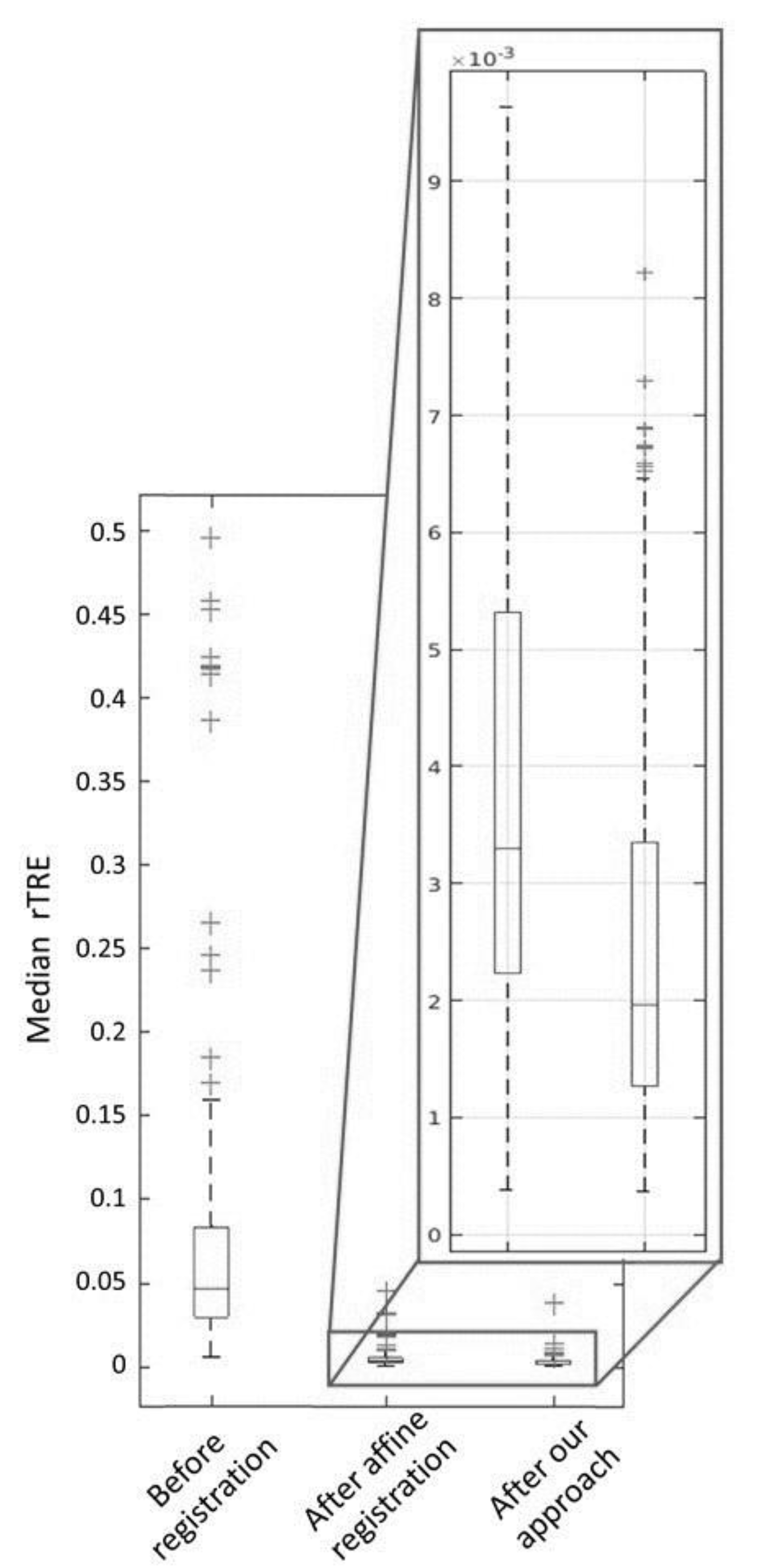
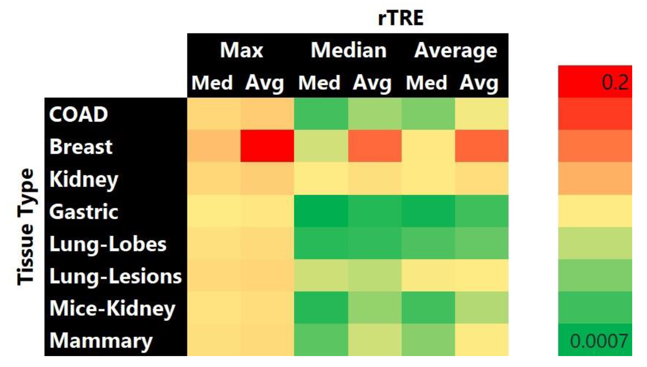
2.5. Evaluation
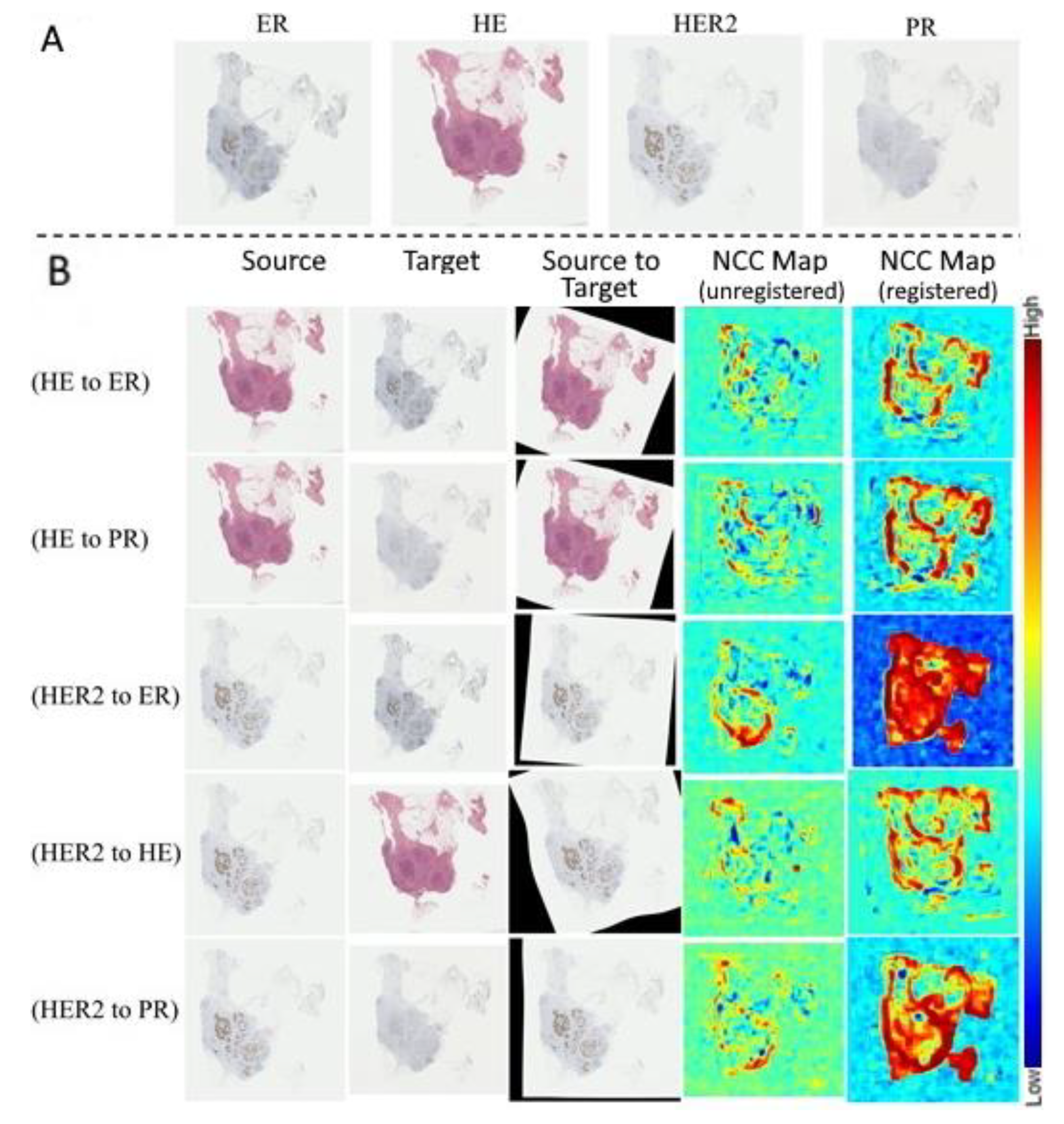
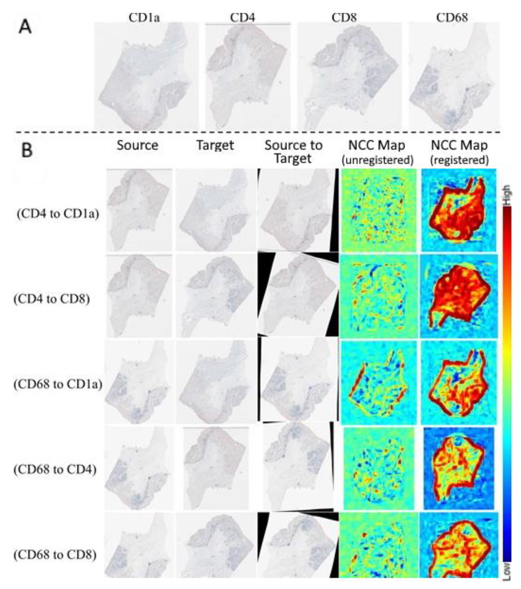
3. Results
4. Discussion
Author Contributions
Funding
Institutional Review Board Statement
Informed Consent Statement
Conflicts of Interest
References
- Bakas, S.; Feldman, M.D. Computational staining of unlabelled tissue. Nat. Biomed. Eng. 2019, 3, 425–426. [Google Scholar] [CrossRef]
- Alho, A.T.D.L.; Hamani, C.; Alho, E.J.L.; da Silva, R.E.; Santos, G.A.B.; Neves, R.C.; Carreira, L.L.; Araújo, C.M.M.; Magalhães, G.; Coelho, D.B.; et al. High thickness histological sections as alternative to study the three-dimensional microscopic human sub-cortical neuroanatomy. Brain Struct. Funct. 2018, 223, 1121–1132. [Google Scholar] [CrossRef]
- Obando, D.F.G.; Frafjord, A.; Øynebråten, I.; Corthay, A.; Olivo-Marin, J.; Meas-Yedid, V. Multi-Staining Registration of Large Histology Images. In Proceedings of the 2017 IEEE 14th International Symposium on Biomedical Imaging (ISBI 2017), Melbourne, Australia, 18–21 April 2017; pp. 345–348. [Google Scholar]
- Cunha, F.; Eloy, C.; Matela, N. Supporting the Stratification of Non-Small Cell Lung Carcinoma for Anti PD-L1 Immunotherapy with Digital Image Registration. In Proceedings of the 2019 IEEE 6th Portuguese Meeting on Bioengineering (ENBENG), Lisbon, Portugal, 22–23 February 2019; pp. 1–4. [Google Scholar]
- Klein, S.; Staring, M.; Murphy, K.; Viergever, M.A.; Pluim, J.P.W. Elastix: A Toolbox for intensity-based medical image registration. IEEE Trans. Med. Imaging 2010, 29, 196–205. [Google Scholar] [CrossRef] [PubMed]
- Borovec, J.; Munoz-Barrutia, A.; Kybic, J. Benchmarking of Image Registration Methods for Differently Stained Histological Slides. In Proceedings of the 25th IEEE International Conference on Image Processing (ICIP), Athens, Greece, 7–10 October 2018; pp. 3368–3372. [Google Scholar]
- Avants, B.B.; Epstein, C.L.; Grossman, M.; Gee, J.C. Symmetric diffeomorphic image registration with cross-correlation: Evaluating automated labeling of elderly and neurodegenerative brain. Med. Image Anal. 2008, 12, 26–41. [Google Scholar] [CrossRef] [PubMed]
- Avants, B.B.; Tustison, N.J.; Song, G.; Cook, P.A.; Klein, A.; Gee, J.C. A reproducible evaluation of ANTs similarity metric performance in brain image registration. NeuroImage 2011, 54, 2033–2044. [Google Scholar] [CrossRef]
- Modat, M.; Ridgway, G.R.; Taylor, Z.A.; Lehmann, M.; Barnes, J.; Hawkes, D.J.; Fox, N.C.; Ourselin, S. Fast free-form deformation using graphics processing units. Comput. Methods Programs Biomed. 2010, 98, 278–284. [Google Scholar] [CrossRef]
- Arganda-Carreras, I.; Sorzano, C.O.S.; Marabini, R.; Carazo, J.M.; Ortiz-de-Solorzano, C.; Kybic, J. Consistent and Elastic Registration of Histological Sections Using Vector-Spline Regularization. In Computer Vision Approaches to Medical Image Analysis; Beichel, R.R., Sonka, M., Eds.; Springer: Berlin/Heidelberg, Germany, 2006; pp. 85–95. [Google Scholar]
- Wodzinski, M.; Skalski, A. Multistep, automatic and nonrigid image registration method for histology samples acquired using multiple stains. Phys. Med. Biol. 2020, 66, 025006. [Google Scholar] [CrossRef]
- Wodzinski, M.; Müller, H. DeepHistReg: Unsupervised deep learning registration framework for differently stained histology samples. Comput. Methods Programs Biomed. 2021, 198, 105799. [Google Scholar] [CrossRef]
- Albu, F. Low Complexity Image Registration Techniques Based on Integral Projections. In Proceedings of the 2016 International Conference on Systems, Signals and Image Processing (IWSSIP 2016), Bratislava, Slovakia, 23–25 May 2016; pp. 1–4. [Google Scholar]
- Nan, A. Image Registration with Homography: A Refresher with Differentiable Mutual Information, Ordinary Differential Equation and Complex Matrix Exponential. Master’s Thesis, University of Alberta, Edmonton, AB, Canada, 2020. [Google Scholar]
- Bradski, G. The OpenCV library. Dr Dobb J. Softw. Tools 2000, 25, 120–125. [Google Scholar]
- Cardona, A.; Saalfeld, S.; Schindelin, J.; Arganda-Carreras, I.; Preibisch, S.; Longair, M.; Tomancak, P.; Hartenstein, V.; Douglas, R.J. TrakEM2 software for neural circuit reconstruction. PLoS ONE 2012, 7, e38011. [Google Scholar] [CrossRef]
- Glocker, B.; Sotiras, A.; Komodakis, N.; Paragios, N. Deformable medical image registration: Setting the state of the art with discrete methods. Annu. Rev. Biomed. Eng. 2011, 13, 219–244. [Google Scholar] [CrossRef] [PubMed]
- Borovec, J.; Kybic, J.; Bušta, M.; Ortiz-de-Solórzano, C.; Muñoz-Barrutia, A. Registration of Multiple Stained Histological Sections. In Proceedings of the 2013 IEEE 10th International Symposium on Biomedical Imaging, San Francisco, CA, USA, 7–11 April 2013; pp. 1034–1037. [Google Scholar]
- Kybic, J.; Borovec, J. Automatic Simultaneous Segmentation and Fast Registration of Histological Images. In Proceedings of the 2014 IEEE 11th International Symposium on Biomedical Imaging (ISBI), Beijing, China, 29 April–2 May 2014; pp. 774–777. [Google Scholar]
- Kybic, J.; Dolejší, M.; Borovec, J. Fast Registration of Segmented Images by Normal Sampling. In Proceedings of the 2015 IEEE Conference on Computer Vision and Pattern Recognition Workshops (CVPRW), Boston, MA, USA, 7–12 June 2015; pp. 11–19. [Google Scholar]
- Awan, R.; Rajpoot, N. Deep Autoencoder Features for Registration of Histology Images; Springer International Publishing: Cham, Switzerland, 2018; pp. 371–378. [Google Scholar]
- Nicolás-Sáenz, L.; Guerrero-Aspizua, S.; Pascau, J.; Muñoz-Barrutia, A. Nonlinear image registration and pixel classification pipeline for the study of tumor heterogeneity maps. Entropy 2020, 22, 946. [Google Scholar] [CrossRef] [PubMed]
- Wodzinski, M.; Müller, H. Unsupervised Learning-Based Nonrigid Registration of High Resolution Histology Images. In International Workshop on Machine Learning in Medical Imaging; Springer: Cham, Switzerland, 2020; pp. 484–493. [Google Scholar]
- Nan, A.; Tennant, M.; Rubin, U.; Ray, N. Drmime: Differentiable Mutual Information and Matrix Exponential for Multi-Resolution Image Registration. In Proceedings of the Third Conference on Medical Imaging with Deep Learning, PMLR, Montreal, QC, Canada, 6–8 July 2020; pp. 527–543. [Google Scholar]
- Alam, F.; Rahman, S.U.; Ullah, S.; Gulati, K. Medical image registration in image guided surgery: Issues, challenges and research opportunities. Biocybern. Biomed. Eng. 2018, 38, 71–89. [Google Scholar] [CrossRef]
- Fernandez-Gonzalez, R.; Jones, A.; Garcia-Rodriguez, E.; Chen, P.Y.; Idica, A.; Lockett, S.J.; Barcellos-Hoff, M.H.; Ortiz-De-Solorzano, C. System for combined three-dimensional morphological and molecular analysis of thick tissue specimens. Microsc. Res. Tech. 2002, 59, 522–530. [Google Scholar] [CrossRef] [PubMed]
- Gupta, L.; Klinkhammer, B.M.; Boor, P.; Merhof, D.; Gadermayr, M. Stain Independent Segmentation of Whole Slide Images: A Case Study in Renal Histology. In Proceedings of the IEEE 15th International Symposium on Biomedical Imaging (ISBI 2018), Washington, DC, USA, 4–7 April 2018; pp. 1360–1364. [Google Scholar]
- Mikhailov, I.; Danilova, N.; Malkov, P. The Immune Microenvironment of Various Histological Types of EBV-Associated Gastric Cancer. In Virchows Archiv; Springer: New York, NY, USA, 2018; Volume 473, p. S168. [Google Scholar]
- Bueno, G.; Deniz, O. AIDPATH: Academia and Industry Collaboration for Digital Pathology. Available online: http://aidpath.eu/?page_id=279 (accessed on 1 August 2020).
- Ruifrok, A.C.; Johnston, D.A. Quantification of histochemical staining by color deconvolution. Anal. Quant. Cytol. Histol. 2001, 23, 291–299. [Google Scholar]
- Schindelin, J.; Arganda-Carreras, I.; Frise, E.; Kaynig, V.; Longair, M.; Pietzsch, T.; Preibisch, S.; Rueden, C.; Saalfeld, S.; Schmid, B.; et al. Fiji: An open-source platform for biological-image analysis. Nat. Methods 2012, 9, 676–682. [Google Scholar] [CrossRef] [PubMed]
- Yushkevich, P.A.; Pluta, J.; Wang, H.; Wisse, L.E.M.; Das, S.; Wolk, D. Fast automatic segmentation of hippocampal subfields and medial temporal lobe subregions in 3 Tesle and 7 Tesla T2-weighted MRI. Alzheimer Dement. J. Alzheimer Assoc. 2016, 12, P126–P127. [Google Scholar] [CrossRef]
- Joshi, S.; Davis, B.; Jomier, M.; Gerig, G. Unbiased diffeomorphic atlas construction for computational anatomy. NeuroImage 2004, 23, S151–S160. [Google Scholar] [CrossRef] [PubMed]
- Yushkevich, P.A.; Piven, J.; Hazlett, H.C.; Smith, R.G.; Ho, S.; Gee, J.C.; Gerig, G. User-guided 3D active contour segmentation of anatomical structures: Significantly improved efficiency and reliability. NeuroImage 2006, 31, 1116–1128. [Google Scholar] [CrossRef]
- Yushkevich, P.A.; Pashchinskiy, A.; Oguz, I.; Mohan, S.; Schmitt, J.E.; Stein, J.M.; Zukić, D.; Vicory, J.; McCormick, M.; Yushkevich, N.; et al. User-guided segmentation of multi-modality medical imaging datasets with ITK-SNAP. Neuroinformatics 2019, 17, 83–102. [Google Scholar] [CrossRef]
- Davatzikos, C.; Rathore, S.; Bakas, S.; Pati, S.; Bergman, M.; Kalarot, R.; Sridharan, P.; Gastounioti, A.; Jahani, N.; Cohen, E.; et al. Cancer imaging phenomics toolkit: Quantitative imaging analytics for precision diagnostics and predictive modeling of clinical outcome. J. Med. Imaging 2018, 5, 011018. [Google Scholar] [CrossRef] [PubMed]
- Rathore, S.; Bakas, S.; Pati, S.; Akbari, H.; Kalarot, R.; Sridharan, P.; Rozycki, M.; Bergman, M.; Tunc, B.; Verma, R.; et al. Brain Cancer Imaging Phenomics Toolkit (brain-CaPTk): An Interactive Platform for Quantitative Analysis of Glioblastoma. Brainlesion: Glioma, Multiple Sclerosis, Stroke and Traumatic Brain Injuries. In Proceedings of the Third International Workshop, BrainLes 2017, Held in Conjunction with MICCAI 2017, Quebec City, QC, Canada, 14 September 2017; pp. 133–145. [Google Scholar]
- Pati, S.; Singh, A.; Rathore, S.; Gastounioti, A.; Bergman, M.; Ngo, P.; Ha, S.M.; Bounias, D.; Minock, J.; Murphy, G.; et al. The Cancer Imaging Phenomics Toolkit (CaPTk): Technical Overview. Brainlesion: Glioma, Multiple Sclerosis, Stroke and Traumatic Brain Injuries; Crimi, A., Bakas, S., Eds.; Springer International Publishing: Cham, Switzerland, 2020; pp. 380–394. [Google Scholar]
- Tsai, D.-M.; Lin, C.-T. Fast normalized cross correlation for defect detection. Pattern Recognit. Lett. 2003, 24, 2625–2631. [Google Scholar] [CrossRef]
- Mokhtari, A.; Ribeiro, A. Global convergence of online limited memory BFGS. J. Mach. Learn. Res. 2015, 16, 3151–3181. [Google Scholar]
- Deriche, R. Fast algorithms for low-level vision. IEEE Trans. Pattern Anal. Mach. Intell. 1990, 12, 78–87. [Google Scholar] [CrossRef]
- Adler, D.H.; Wisse, L.E.M.; Ittyerah, R.; Pluta, J.B.; Ding, S.L.; Xie, L.; Wang, J.; Kadivar, S.; Robinson, J.L.; Schuck, T.; et al. Characterizing the human hippocampus in aging and Alzheimer’s disease using a computational atlas derived from ex vivo MRI and histology. Proc. Natl. Acad. Sci. USA 2018, 115, 4252–4257. [Google Scholar] [CrossRef]
- Borovec, J.; Kybic, J.; Arganda-Carreras, I.; Sorokin, D.V.; Bueno, G.; Khvostikov, A.V.; Bakas, S.; Chang, E.I.-C.; Heldmann, S.; Kartasalo, K.; et al. ANHIR: Automatic Non-Rigid Histological Image Registration Challenge. IEEE Trans. Med. Imaging 2020, 39, 3042–3052. [Google Scholar] [CrossRef]
- Borovec, J.; Kybic, J.; Muñoz-Barrutia, A. Automatic Non-Rigid Histological Image Registration Challenge—Statistics. In Proceedings of the IEEE International Symposium on Biomedical Imaging (ISBI), Venice, Italy, 8–11 April 2019. [Google Scholar]
- Shin, D. User perceptions of algorithmic decisions in the personalized AI system: Perceptual evaluation of fairness, accountability, transparency, and explainability. J. Broadcasting Electron. Media 2020, 13, 1–25. [Google Scholar]
- Shin, D. The effects of explainability and causability on perception, trust, and acceptance: Implications for explainable AI. Int. J. Hum. Comput. Stud. 2021, 146, 102551. [Google Scholar] [CrossRef]
- Bakas, S.; Doulgerakis-Kontoudis, M.; Hunter, G.J.; Sidhu, P.S.; Makris, D.; Chatzimichail, K. Evaluation of indirect methods for motion compensation in 2-D focal liver lesion contrast-enhanced ultrasound (CEUS) imaging. Ultrasound Med. Biol. 2019, 45, 1380–1396. [Google Scholar] [CrossRef]
- Yushkevich, P.A.; Avants, B.B.; Ng, L.; Hawrylycz, M.; Burstein, P.D.; Zhang, H.; Gee, J.C. 3D Mouse Brain Reconstruction from Histology Using a Coarse-to-Fine Approach. Biomedical Image Registration; Pluim, J.P.W., Likar, B., Gerritsen, F.A., Eds.; Springer: Berlin/Heidelberg, Germany, 2006; pp. 230–237. [Google Scholar]
- Adler, D.H.; Pluta, J.; Kadivar, S.; Craige, C.; Gee, J.C.; Avants, B.B.; Yushkevich, P.A. Histology-derived volumetric annotation of the human hippocampal subfields in postmortem MRI. NeuroImage 2014, 84, 505–523. [Google Scholar] [CrossRef]
- Bakas, S.; Akbari, H.; Pisapia, J.; Martinez-Lage, M.; Rozycki, M.; Rathore, S.; Dahmane, N.; O’Rourke, D.M.; Davatzikos, C. In vivo detection of EGFRvIII in glioblastoma via perfusion magnetic resonance imaging signature consistent with deep peritumoral infiltration: The φ-index. Clin. Cancer Res. 2017, 23, 4724–4734. [Google Scholar] [CrossRef]
- Akbari, H.; Bakas, S.; Pisapia, J.M.; Nasrallah, M.P.; Rozycki, M.; Martinez-Lage, M.; Morrissette, J.J.D.; Dahmane, N.; O’Rourke, D.M.; Davatzikos, C. In vivo evaluation of EGFRvIII mutation in primary glioblastoma patients via complex multiparametric MRI signature. Neuro Oncol. 2018, 20, 1068–1079. [Google Scholar] [CrossRef] [PubMed]
- Binder, Z.A.; Thorne, A.H.; Bakas, S.; Wileyto, E.P.; Bilello, M.; Akbari, H.; Rathore, S.; Ha, S.M.; Zhang, L.; Ferguson, C.J.; et al. Epidermal growth factor receptor extracellular domain mutations in glioblastoma present opportunities for clinical imaging and therapeutic development. Cancer Cell 2018, 34, 163–177. [Google Scholar] [CrossRef] [PubMed]
- Elsheikh, S.S.M.; Bakas, S.; Mulder, N.J.; Chimusa, E.R.; Davatzikos, C.; Crimi, A. Multi-Stage Association Analysis of Glioblastoma Gene Expressions with Texture and Spatial Patterns. Brainlesion: Glioma, Multiple Sclerosis, Stroke and Traumatic Brain Injuries; Crimi, A., Bakas, S., Kuijf, H., Keyvan, F., Reyes, M., van Walsum, T., Eds.; Springer International Publishing: Cham, Switzerland, 2019; pp. 239–250. [Google Scholar]
- Yagi, Y.; Riedlinger, G.; Xu, X.; Nakamura, A.; Levy, B.; Iafrate, A.J.; Mino-Kenudson, M.; Klepeis, V.E. Development of a database system and image viewer to assist in the correlation of histopathologic features and digital image analysis with clinical and molecular genetic information. Pathol. Int. 2016, 66, 63–74. [Google Scholar] [CrossRef] [PubMed]


Publisher’s Note: MDPI stays neutral with regard to jurisdictional claims in published maps and institutional affiliations. |
© 2021 by the authors. Licensee MDPI, Basel, Switzerland. This article is an open access article distributed under the terms and conditions of the Creative Commons Attribution (CC BY) license (http://creativecommons.org/licenses/by/4.0/).
Share and Cite
Venet, L.; Pati, S.; Feldman, M.D.; Nasrallah, M.P.; Yushkevich, P.; Bakas, S. Accurate and Robust Alignment of Differently Stained Histologic Images Based on Greedy Diffeomorphic Registration. Appl. Sci. 2021, 11, 1892. https://doi.org/10.3390/app11041892
Venet L, Pati S, Feldman MD, Nasrallah MP, Yushkevich P, Bakas S. Accurate and Robust Alignment of Differently Stained Histologic Images Based on Greedy Diffeomorphic Registration. Applied Sciences. 2021; 11(4):1892. https://doi.org/10.3390/app11041892
Chicago/Turabian StyleVenet, Ludovic, Sarthak Pati, Michael D. Feldman, MacLean P. Nasrallah, Paul Yushkevich, and Spyridon Bakas. 2021. "Accurate and Robust Alignment of Differently Stained Histologic Images Based on Greedy Diffeomorphic Registration" Applied Sciences 11, no. 4: 1892. https://doi.org/10.3390/app11041892
APA StyleVenet, L., Pati, S., Feldman, M. D., Nasrallah, M. P., Yushkevich, P., & Bakas, S. (2021). Accurate and Robust Alignment of Differently Stained Histologic Images Based on Greedy Diffeomorphic Registration. Applied Sciences, 11(4), 1892. https://doi.org/10.3390/app11041892