Article

From Traffic-Channeling Gateway to Versatile Bargaining Ability: Strategic Channel Governance and Sustainable Cooperation in Live Stream E-Commerce


School of Management, Xi’an Jiaotong University, Xi’an 710049, China
*
Author to whom correspondence should be addressed.
J. Theor. Appl. Electron. Commer. Res. 2026, 21(8), 259; https://doi.org/10.3390/jtaer21080259
Submission received: 31 May 2026 / Revised: 23 July 2026 / Accepted: 24 July 2026 / Published: 5 August 2026

Abstract

In the burgeoning live stream landscape, manufacturers face critical dilemmas regarding strategic channel governance and how intermediaries’ bargaining ability dictates sustainable cooperation under Stackelberg leadership change. Addressing these issues is vital, as misaligned governance risks severe profit losses, yet standard heuristics fail to capture how leadership shifts disrupt channel coordination and model selection. To fill this gap, we model a manufacturer’s self-operated (Model SO) live stream channel and an intermediary-operated (Model IO) live stream channel to evaluate trade-offs among bargaining ability, operational costs, and spillover effects. Key findings show that in Model SO, spillover and price adjustments transform the live stream channel into a traffic-channeling gateway in which rising operational costs paradoxically boost total profits. In Model IO, bargaining ability serves as a key determinant, as high pit fees weaponize this ability for predatory commission-squeezing, while low pit fees redirect it toward volume expansion, transforming the intermediary into a synergistic partner. Furthermore, bargaining ability shifts pricing from intermediary-introduction to profit-recapture strategies while exerting cost-magnification and revenue-magnification effects under varying pit fees. Crucially, we uncover two Pareto-optimal cooperation zones alongside a non-cooperation zone caused by incentive incompatibility under mid-tier bargaining ability. Extensions show that intensified price competition turns dominant intermediaries into welfare killers and high service sensitivity induces an over-service trap, though popularity cost-sharing contracts restore coordination. Overall, this study fills a crucial analytical gap by establishing precise theoretical boundaries for channel governance, bargaining ability dynamics, and cost-driven functional transformations in live stream supply chains.

1. Introduction

In the evolving dual-channel supply-chain landscape, live stream e-commerce has emerged as a transformative force, reshaping traditional channel governance and facilitating business cooperation [1]. Global live stream e-commerce sales are projected to reach USD 3.93 billion by 2030, with a CAGR of 21.9% from 2025–2030 [2]. This industry has evolved from a supplemental sales tool into a multi-trillion-dollar market. To capitalize on this trend, manufacturers typically navigate two distinct strategic paths [3,4]. One is that they establish self-operated live stream teams to maintain direct control over promotion and pricing [5]. In practice, we have witnessed numerous manufacturers and brand owners, such as the fashion brand Zara [6], start self-operated live streams to sell products during the past several years on both e-commerce and social platforms. The other way is to outsource the live stream selling task to third-party intermediaries, such as KOLs, to leverage their professional influence [7]. According to the statistics, in 2026, there will be a total of 650 million active live streaming viewers in China, 22 million registered live-streamers and a 12% annual increase in the growth rate of the live stream industry [8].
However, as manufacturers dive deeper into these operations, several counter-intuitive phenomena have begun to surface that challenge traditional supply-chain logic. In the manufacturers’ self-operated live streams, we have witnessed many manufacturers aggressively ramping up their promotion intensity even as live stream operational costs soar [9]. Why would rational firms double down on a seemingly loss-making channel? This strategic choice suggests that the live stream channel may be undergoing a functional transformation, moving beyond a simple sales outlet. Instead of just selling products, it may act as a tool to drive traffic to traditional channels, a mechanism that is still not fully understood.
The narrative becomes more complex in the intermediary-operated live stream, where the intermediary’s bargaining ability is the most critical factor [10]. In industrial practice, this bargaining ability does not just affect commissions [11], it also helps the intermediary attract more traffic [12]. Powerful intermediaries use their positions to secure exclusive resource access (e.g., product premieres) and brand-funded promotional support (e.g., lucky-draw prizes and co-marketing traffic) [13]. Because of the intermediaries’ strong bargaining ability, they personally bear the traffic costs and convert traffic into sales with high efficiency. Consequently, manufacturers can leverage this lower traffic cost advantage to capture significantly higher sales and profits through the live stream room [14]. However, while some partnerships increase total supply-chain profits, others fail because excessive pit fees or commissions severely hurt the manufacturer [15]. This raises a critical question: how does the intermediary’s bargaining ability affect sustainable cooperation and promotion decisions, and what is the exact boundary where this cooperation remains profitable for the manufacturer?
This complexity is also reflected in the shifts in supply-chain leadership. The manufacturer acts as the Stackelberg leader in a self-operated live stream, but otherwise cedes this leadership to the intermediary [16,17]. However, prior analytical models [3,5,18,19] heavily rely on static, manufacturer-led structures, leaving a critical gap in how such leadership reversal interacts with the intermediary’s bargaining ability, operational costs, and channel spillovers [20,21,22,23]. In practice, prominent mega-streamers and MCNs have built extensive traffic ecosystems and independent supply chains (e.g., top-tier streamers like Austin Li’s “MeiOne,” XinBa’s “Xin Select” and Luo Yonghao’s “Make a Friend”), gathering substantial channel power as Stackelberg leaders. Driven by both this widespread industry practice and the lack of attention in the existing literature, examining Stackelberg leadership shifts is essential to fill the gap. This analysis not only contributes new theoretical insights and methodologies to the literature, but also provides actionable guidance for industry practitioners.
Furthermore, the existing e-commerce literature reveals that bargaining ability is often modeled with a single function, typically serving only as a fixed profit-sharing ratio parameter between supply-chain participants [22,23,24,25]. It fails to capture the multidimensional impacts of bargaining ability on endogenous commissions and traffic acquisition. Addressing these literature gaps is theoretically and managerially significant for two key reasons. First, oversimplifying bargaining ability as a static profit-split parameter overlooks its operational role in driving traffic and determining commission rates. It can lead practitioners to misjudge channel profitability and misallocate promotional budgets. Second, evaluating bargaining ability under leadership shifts is vital because channel dynamics fundamentally change when the intermediary leads, determining whether strong intermediaries act as predatory profit squeezers or synergistic growth drivers. To resolve these issues, a formal game-theoretic framework is necessary because conventional intuition and simplified baseline models fail to capture the underlying interactions. Standard heuristics assume that rising operational costs consistently erode profits or that stronger intermediary power always hurts manufacturers. However, formal analytical modeling is required to derive the non-monotonic trade-offs between pit fees, spillover effects, and leadership structures, thereby establishing exact analytical boundaries for sustainable channel cooperation. Motivated by these industry observations and research gaps, we address the following research questions:
(1)
How does the strategic positioning of a live stream channel evolve within a dual-channel supply chain?
(2)
How does the intermediary’s bargaining ability affect the optimal pricing, supply-chain performance, welfare and other key decision variables?
(3)
Considering the intermediary’s bargaining ability, live stream operational cost, and channel spillover effects, what are the equilibrium boundaries for governance-optimal live stream model selection, and for cooperation or non-cooperation zones between the manufacturer and the intermediary?
(4)
How do negative popularity spillover and consumer channel preference affect the manufacturer’s strategic decisions? How can one properly design cost-sharing and a live stream support mechanism so the manufacturer avoids the “over-service trap”?
To answer these questions, we construct game models within a dual-channel framework to compare a manufacturer-operated live stream (Model SO) and an intermediary-operated live stream (Model IO). We incorporate the positive effects of both promotion efforts and the intermediary’s popularity on demand. Model SO features a manufacturer-led Stackelberg game, while Model IO shifts the leadership to the intermediary. By deriving and comparing the equilibrium solutions, we identify how key parameters influence pricing, promotion decisions, and member profits under both models. Furthermore, we design Pareto-improvement mechanisms to explore the conditions for win–win cooperation. Finally, we extend our core models to analyze consumer surplus, channel spillovers, cost-sharing contracts, and over-service issues.
Several key findings can be drawn from this study. First, in Model SO, the live stream serves as a “traffic-channeling gateway” to redirect traffic to the more profitable retail channel via price adjustments and spillover effects. In Model IO, high pit fees lead to high commissions that hurt the manufacturer, while low pit fees align both parties toward sales expansion. Second, a stronger bargaining ability is a double-edged sword; it can magnify costs rather than revenues, depending on the cost structure. Third, supply-chain leadership and bargaining ability drive pricing differentials. We map two Pareto-optimal cooperation zones with low/high bargaining ability intermediaries and show that cooperation always fails with a mid-tier bargaining ability intermediary. Lastly, intense cross-channel competition can cause social welfare losses, and high consumer sensitivity triggers a profit-eroding over-service trap, which can be resolved by an optimal cost-sharing contract.
This study offers several key theoretical and managerial contributions. First, we extend multi-channel governance theory by showing that a live stream channel can be strategically re-positioned as a traffic-channeling gateway that subsidizes reselling channels. Second, multifaceted impacts of bargaining ability are identified. Unlike the existing literature that views a third party’s bargaining ability as a static threat [25], we show that its impact is contingent on the contract structure. Bargaining ability can be weaponized for predatory extraction under high pit fees or redirected for coordination and sales expansion under low pit fees. We also show that while top-tier intermediaries expand market reach, they can reduce social welfare in highly competitive markets. Third, we prove that cross-channel pricing differentials are driven by bargaining ability rather than operational costs alone, establishing a more comprehensive pricing framework. Finally, we define the clear governance boundaries between the two models by mapping the exact Pareto-optimal cooperation zones. In doing so, this study clearly provides intuitive baseline dynamics from non-trivial analytical discoveries. We demonstrate that formal game-theoretic modeling is indispensable for identifying the precise boundary conditions, such as the unexpected failure of cooperation under mid-tier bargaining ability, where intuitive expectations fail to hold. Our results provide actionable guidance for managers to avoid mid-tier intermediaries where incentives are misaligned, and warn firms against an over-service trap where excessive investment erodes profits.
The remainder of this paper is arranged as follows. Section 2 reviews the related literature. Section 3 presents theoretical models and equilibrium analysis. Section 4 analyzes optimal pricing and key decisions for the manufacturer and the intermediary. Section 5 extends models to provide more insights and test the robustness of our main model. Section 6 discusses theoretical and managerial implications, concluding with remarks and a discussion of the limitations.

2. Literature Review

Our study is related to three areas in the literature, namely, (i) dual-channel operations; (ii) promotion strategies and service investment; and (iii) live stream selling. We provide a review of some related studies as follows.

2.1. Dual-Channel Operations

The classic dual-channel literature typically assumes that each channel aims to maximize its own profit and maintains an independent marginal contribution [26,27]. For example, Tsay and Agrawal [28] explored channel conflict between independent profit-seeking entities, identifying inefficiencies from double marginalization and unperceived sales externalities. Chiang et al. [29] examined direct channels as strategic threats operating to constrain retail pricing and mitigate double marginalization, primarily focusing on price-driven competition rather than those utilizing the channel as a synergistic traffic driver.
Additionally, the dual-channel literature also extensively discusses showrooming and webrooming [30,31], exploring the spillover effects [20,32] between e-commerce channels and the reactive strategies of market members. Some studies suggest that spillover effects can be beneficial for improving services and reducing pricing. For instance, Chen et al. [33] studied how the showrooming effect influences pricing strategies and channel performance in dual-channel supply chains under three distinct power structures. Li et al. [34] investigated how showrooming effects and service timing influence dual-channel performance, demonstrating that ex post service strategies with low wholesale prices can, paradoxically, enhance profits for both entities. Conversely, other research argues that the spillover effects are detrimental. Balakrishnan et al. [35] demonstrated that showrooming harms retailers by intensifying price competition between dual-channels and allowing online channels to free-ride on costly offline services. However, these studies generally assume that showrooming or webrooming is driven by consumer behavior, forcing supply-chain members to react passively to varying effects.
The existing literature on dual-channel supply chains in e-commerce predominantly treats individual channels as static and independent profit centers [36]. There is a lack of quantitative analysis regarding the logic of sacrificing single-channel profitability to positively drive aggregate traffic growth across the entire ecosystem. Diverging from traditional paradigms, our study adds to the literature in two ways. First, we break the “independent profit center” assumption [26,27,28,29,36] by introducing a low-margin live stream channel as a traffic-channeling gateway. Second, unlike studies treating spillovers as passive consumer behavior [20,32,33,34,35], we prove manufacturers can proactively manage spillovers for ecosystem-wide value creation.

2.2. Promotion Strategies and Service Investment

One stream of the marketing and supply-chain literature establishes the foundational logic that channel spillovers, sales efforts and promotional investments are positively correlated with demand [37,38]. In particular, Zhang et al. [39] empirically demonstrated that there is a positive cross-channel spillover effect from the live stream shopping to the online store channel, increasing the revenue of the latter in one case by 46.2%. Huang and Morozov [40] examined how live video game streaming affects game popularity, using minute-level viewership data from 60,000 Twitch.tv streamers over eight months. Kumar et al. [41] investigated the critical components of metaverse advertising and their impacts on promotional effectiveness through analysis of netizens’ first-hand experiences. Zhang et al. [13] examined the longitudinal effects of lucky-draw promotions by comparing pre-adoption, active-promotion, and post-promotion sales performance in live stream commerce. Niu et al. [7] evaluated the efficacy of key opinion leader (KOL) promotions for brand owners operating both direct-selling and traditional retail channels. Schamp et al. [42] provided the first large-scale field analysis of cause-related marketing promotions (CMPs), offering actionable guidelines for tailoring CMP strategies to brand and category contexts.
Another significant body of work focuses on service competition within dual-channel structures. These studies often characterize service as a competitive weapon, where firms engage in a “service race” to differentiate themselves. Wei and Shao [43] demonstrated that platform retail service investment universally benefits both platforms and manufacturers, creating win–win outcomes under high spillover effects while influencing manufacturers’ strategic selections of live stream modes. Amankou et al. [44] advocated for increasing technical service investments in dual-channel retail, demonstrating that BIIoT-based essential services can significantly drive demand and enhance manufacturing profits by 29.12%. Zhou et al. [27] examined service-cost sharing contracts in dual-channel chains with free-riding, demonstrating that while such contracts stimulate service levels, pricing scenarios significantly dictate profit distribution between members. However, there is a notable scarcity of research investigating whether such competitive races can evolve into a trap that actively erodes total profitability rather than merely increasing costs.
Our study extends the promotion strategy literature [15,16,17,18,19,23] by classifying purchased traffic into two distinct forms, autonomous promotion and intermediary popularity. It proves power structures dictate how firms use such purchases as strategic tools. Furthermore, challenging the theory that investment increases profits, we identify an over-service trap arising due to consumer sensitivity to services. This establishes a critical negative feedback boundary for e-commerce promotion and service theory.

2.3. Live Stream Selling

Early live stream selling research applied empirical methods to study purchase decisions [45,46]. Sun et al. [47] examined how IT affordances (visibility, meta-voicing, and guidance) boost engagement and purchases. Lu and Chen [48] found broadcaster traits reduce uncertainty, enhancing trust and sales in fashion markets. Recent studies explore streamers’ impacts on sales [18,49,50,51], sales mode selection [52,53,54], and channel strategies [55,56,57,58]. Guo et al. [59] showed affective call-to-actions boost purchases, while cognitive ones reduce interactions. Gu et al. [60] found big influencers expand reach, whereas small ones increase conversions. While research in live stream selling is growing, it often centers on consumer behavior, the personal characteristics of streamers, and channel management. Although some studies address bargaining ability, they typically view it as a one-dimensional tool for profit extraction [24].
The study most relevant to our work is that by Chen et al. [24]. The authors examined how streamers’ bargaining power influences merchants’ selection between traditional and live e-commerce, revealing that while moderate bargaining power facilitates win–win outcomes, excessive power erodes merchant profits and social welfare through high pit fees. Unlike Chen et al. [24], who studied single-channel selection with a unified leader, our work examines dual-channel competition between two live stream models under shifting Stackelberg leadership. While they find moderate bargaining power optimal, we reveal the opposite outcome, that such power triggers incentive incompatibility due to leadership change. We thus enrich the literature by demonstrating how structural power dynamics and multi-party leadership fundamentally reshape the live stream selling landscape.
To address what this study adds to existing knowledge, our results enrich the live stream literature in three ways. First, we prove that shifting leadership causes cooperation to fail under moderate bargaining ability. Second, extending traditional views of bargaining ability as a static threat, we show its nature is contingent on pit fees and popularity acquisition costs. Finally, we introduce the over-service trap phenomenon, establishing a negative feedback boundary for live stream investments. To highlight the position of this paper in the literature, the major differences between our paper and the existing studies are summarized in Table 1.

3. Model

3.1. Model Formation

Consider a dual-channel supply chain consisting of a manufacturer, a reseller, and an intermediary. The manufacturer sells products via a traditional retail channel and a live stream channel. In the retail channel, the manufacturer sells goods to the reseller at a wholesale price, who then sets the retail price for consumers. The live stream channel involves two primary modes: First, there is the manufacturer’s self-operated live stream (Model SO), where the manufacturer directly manages live stream operations. Second, there is the intermediary-operated live stream (Model IO), where operations are outsourced to an intermediary. These represent the predominant industry modes and are widely studied in the literature [3,19,24]. Notably, we investigate the Stackelberg leadership shifts from the manufacturer to the intermediary under Model IO, which is commonly used in the previous literature [66,67]. This modeling choice captures the dramatic power shift in contemporary e-commerce, where top-tier live-streamers switch from being plain promotional channels to critical supply-chain governors. In real-world industry practice, leading intermediaries, top-tier MCN institutions, and celebrity streamers possess absolute gatekeeping power and control consumer traffic routing within the e-commerce ecosystem. For instance, top streamers like Austin Li often demand exclusive pricing rights (e.g., “lowest price across the entire network”). Consequently, these mega-intermediaries often dictate pricing structures, pit fees, and promotion schedules, forcing traditional brands into a follower position where they can only react to the intermediary’s decisions. Therefore, by choosing Model IO, the manufacturer acknowledges the intermediary’s superior resource endowment and traffic operations, which grants the intermediary the position of Stackelberg leader.
Without the loss of generality, we normalize production cost to zero [63,68]. Following Wang et al. [64], we omit the influencer’s sales effort, treating it as a standardized baseline, to isolate the impacts of bargaining ability and traffic costs. Additionally, for model traceability, the platform’s exogenous commission rate is excluded [69,70] because platforms typically apply uniform commission rates to products within the same category regardless of the seller’s identity. This allows us to assume the platform acts as a neutral infrastructure provider, and to focus strictly on the leadership dynamics and better investigating strategic interactions between the manufacturer and the intermediary.
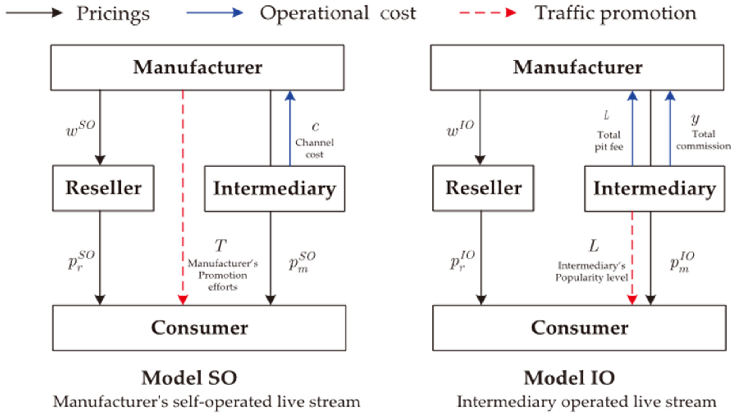
Methodologically, it is worth noting that our analytical framework contributes to the live stream e-commerce and channel governance literature by refining how operational structures and power dynamics are represented in game-theoretic models. Specifically, we address three critical gaps. First, while existing models often simplify live-stream channels with exogenous commission rates and ignore upfront building costs [71], we endogenize these cost variables to capture the realistic trade-off between fixed entry costs and variable commissions. Second, unlike prior studies that assume static game leadership with the manufacturer as a permanent Stackelberg leader [43,49,71], our model introduces dynamic leadership transitions to reflect real-world industrial power shifts. Third, we innovatively integrate bargaining ability with both commission negotiations and popularity acquisition to capture its dual function, a phenomenon widely observed in practice but rarely modeled. Ultimately, by combining dynamic leadership transitions with multidimensional bargaining ability, our framework provides a comprehensive methodological approach that captures the complex interactions between game structures and negotiation capabilities. The dual-channel supply-chain structure is presented in Figure 1, and notations and parameters are listed in Table 2. Long thresholds used in the article are summarized in Table A1 in Appendix A.

3.1.1. Model SO—Manufacturer’s Self-Operated Live Stream

In Model SO, the intermediary is vertically integrated and serves purely as a marketplace, providing channel infrastructure and technical support in exchange for an exogenous channel fee c [72]. Within this framework, the manufacturer supplies products to the reseller at a wholesale price w S O , and the reseller subsequently sells them to consumers at price p r S O . Simultaneously, the manufacturer sells directly to consumers through the live stream channel at retail price p m S O . To increase product exposure and drive sales volume, the manufacturer exerts promotion effort T in the live stream space, incurring a cost of b T 2 / 2 , where b denotes the unit cost of promotion effort [7]. For the convenience of model traceability, the market potential is assumed to be 1 [64]. The demand functions are
q r S O = 1 p r S O + t p m S O + k T q m S O = 1 p m S O + t p r S O + T
k denotes positive spillover effect into the reselling channel, a determination which is commonly used in the previous literature [32,62]. This parameter reflects the “billboard effect” of a live stream. Even if consumers do not buy directly in the live stream room, the intense product exposure and high-frequency demonstrations significantly amplify brand awareness, thereby boosting organic traffic and demand in the traditional channel. t represents cross-channel price competition intensity [33]. The profit functions for the supply-chain members are as follows:
max π m S O ( w S O , p m S O , T ) = w S O ( 1 p r S O + t p m S O + k T ) + ( p m S O c ) ( 1 p m S O + t p r S O + T ) b T 2 2 max π r S O ( p r S O ) = ( p r S O w S O ) ( 1 p r S O + t p m S O + k T ) π I S O = c ( 1 p m S O + t p r S O + T )
The sequence of events in Model SO is as follows: In stage 1, acting as the Stackelberg leader, the manufacturer simultaneously determines the wholesale price w S O , the live stream retail price p m S O , and the promotion effort level T . In stage 2, the reseller determines the retail price p r S O for the reselling channel based on the manufacturer’s decisions. To ensure all equilibrium results are positive, we make the following assumptions in Model SO: 0 < c < c , b < b c > c , 0 < b < b where c = k t + k + 2 k t k t 2 2 t + 2 , b = k 2 t 2 + k 2 + 4 k t + 2 4 ( 1 t 2 ) . The equilibrium results for Model SO are listed in Table 3.

3.1.2. Model IO—Intermediary-Operated Live Stream

In Model IO, the manufacturer outsources the live stream sales operations to an intermediary. The intermediary possesses a bargaining ability [24,25], denoted by y . We model this parameter from the real-world practice to reflect an intermediary’s professional negotiation leverage and traffic acquisition efficiency. The bargaining ability generates two distinct effects. First, regarding popularity acquisition, the intermediary is responsible for acquiring popularity in the live stream room. Let L represent the popularity level and τ denote unit popularity acquisition cost. Then, the total popularity acquisition cost is defined as τ L 2 / 2 y . With the same level of popularity, the higher the intermediary’s bargaining ability, the less the acquisition cost, which is a common assumption in the previous literature [73,74,75]. Second, the intermediary negotiates the commission with the manufacturer; a higher bargaining ability allows the intermediary to secure a higher total commission, a common assumption in the previous literature [68]. We denote the intermediary’s total commission as y β , where β is the unit commission [24]. Additionally, the manufacturer pays a total pit fee based on the intermediary’s popularity level, denoted as δ L , where δ represents the exogenous unit pit fee [24]. Consistent with Wang et al. [64], this contract setting (compared with fixed pit-fee) strictly mirrors real-world live stream practice, where manufacturers look for the appropriate intermediary by paying pit fees according to popularity.
Consequently, while considering cooperation, the manufacturer must navigate a tradeoff between the reduced unit popularity acquisition costs and the corresponding increases in commission and pit fees facilitated by the intermediary’s bargaining ability. Simultaneously, the intermediary must consider that excessive levels of β and L may lead to a breakdown in cooperation or the erosion of profits due to high total acquisition costs. Following existing frameworks, the demand function for this scenario is derived as follows:
q r I O = 1 p r I O + t p m I O + ρ L q m I O = 1 p m I O + t p r I O + L
ρ denotes the positive spillover effect of popularity to the reselling channel. Note that we will discuss negative spillover effect in the Extensions, below. t represents cross-channel price competition intensity. The profit functions for the supply-chain members are as follows:
max π m I O ( w I O , p m I O ) = w I O ( 1 p r I O + t p m I O + ρ L ) + ( p m I O y β ) ( 1 p m I O + t p r I O + L ) δ L max π r I O ( p r I O ) = ( p r I O w I O ) ( 1 p r I O + t p m I O + ρ L ) max π I I O ( β , L ) = y β ( 1 p m I O + t p r I O + L ) + δ L τ L 2 2 y
The sequence of events in Model IO is as follows: In stage 1, acting as the Stackelberg leader, the intermediary simultaneously determines the unit commission β and the popularity level L . In stage 2, the manufacturer determines the wholesale price w I O and the live stream retail price p m I O based on the intermediary’s decisions. In stage 3, the reseller determines the retail price p r I O for the retail channel, based on the manufacturer’s decisions. To ensure all equilibrium results are positive, we make the following assumptions in Model IO: { τ > τ 2 } { δ < min { δ 1 , δ 2 , δ 3 } , τ < min { τ 1 , τ 3 , τ 4 } } where τ 1 = ρ 2 t y 8 δ ρ y 8 δ t y + ρ t y 2 ρ y + 2 y 8 + 8 t ; τ 2 = ρ 2 t 2 y 4 ρ t y 4 y 8 t 2 16 ; τ 3 = ρ 2 t 2 y ρ t 2 y + 2 ρ t y 2 t y 12 t 3 + 16 t 2 20 t 24 ; τ 4 = 2 ρ 2 t 3 y 2 ρ t 3 y 3 ρ 2 t y + 4 ρ t 2 y + 3 ρ t y 4 t 2 y 6 ρ y + 6 y 2 t 4 12 t 3 18 t 2 + 20 t + 24 ; δ 1 = ρ 2 t + ρ t 2 ρ + 2 8 ρ + 8 t ; δ 2 = ρ 2 t 2 y ρ t 2 y 12 t 3 τ + 2 ρ t y 16 t 2 τ + 20 t τ 2 t y + 24 τ 12 ρ t 3 y 20 ρ t y + 16 t 2 y 24 y ; and δ 3 = 2 ρ 2 t 3 y 2 ρ t 3 y 2 t 4 τ 3 ρ 2 t y + 4 ρ t 2 y + 12 t 3 τ + 3 ρ t y + 18 t 2 τ 4 t 2 y 6 ρ y 20 t τ 24 τ + 6 y 2 ρ t 4 y 18 ρ t 2 y 12 t 3 y + 24 ρ y + 20 t y . The equilibrium results for Model IO are listed in Table 4.
Θ = 4 ρ 2 δ ρ 10 δ t 6 + 8 ρ δ ρ 2 20 δ + 3 ρ t 5 + ρ 4 + 4 δ 2 ρ 3 + 120 δ 2 + 64 δ + 1 ρ 2 + 32 ρ δ 96 δ 2 t 4 + 8 δ + 1 2 ρ 2 + 5 δ 1 ρ + 76 δ 2 + 16 δ + 1 2 ρ t 3 128 δ + 1 4 2 ρ 2 + 64 δ + 16 ρ 320 δ 2 64 δ 8 + 2 ρ 4 + 4 ρ 3 + 16 δ 2 48 δ + 2 ρ 2 + 48 δ 8 ρ + 352 δ 2 + 64 δ + 4 t 2 + 32 δ 8 ρ 3 + 32 δ + 16 ρ 2 + 576 δ 2 160 δ 8 ρ + 32 δ t
Θ 1 = 16 τ t + 1 t 2 2 δ ρ 16 δ t 3 + δ ρ + 16 δ + 2 t 2 + ρ 2 + 2 δ 1 ρ + 32 δ 2 + 10 δ t + 8 δ + 2 ρ 32 δ 2 4 δ 2 y   8 τ 2 t + 1 t 2 2 t 3 + 3 t 2 8 t 12

3.2. Equilibrium Analysis

In this section, we analyze the sensitivity of key factors, such as pricing, promotion efforts, commissions, popularity, and profits, to equilibrium results under both Model SO and Model IO. By examining these relationships, we derive insightful findings and provide corresponding theoretical and managerial implications.

3.2.1. Equilibrium Analysis of Model SO

Lemma 1. 
The effects of key factors on optimal pricing of the manufacturer and the reseller in Model SO are as follows: (i) { w S O * , p r S O * } k > 0   if   { b < b , c > max { c 1 , c 2 } } < 0   if   { b < b , c < min { c 1 , c 2 } }   , p m S O * k > 0   if   b > b , c < c   < 0   if   b < b , c > c ; (ii) { w S O * , p r S O * , p m S O * } b > 0   if   c > c   < 0   if   c < c   ; (iii) { w S O * , p r S O * , p m S O * } c > 0   if   b < b < 0   if   b < b < min { b 1 , b 2 } > 0   if   b > max { b 1 , b 2 } . b = k 2 t 2 k 2 4 k t 2 4 t 2 4 , b 1 = 2 k 2 t 2 k 2 7 k t 4 4 t 2 4 , b 2 = 2 k 2 t 2 k t 2 3 k 3 t 2 t 3 2 t , c = k t k 2 k t 2 k t + 2 t 2 , c 1 = k 2 t 3 8 b k t 2 4 b t 3 + 2 k 2 t 2 16 b k t 8 b t 2 + k 2 t + 4 k t 2 8 b k 12 b t 2 k 2 + 4 k t 8 b + 4 k + 6 t + 4 k 2 t 4 + 8 b k t 3 + 4 b t 4 + k 2 t 2 4 k t 3 8 b k t + 4 b t 2 2 k 2 6 t 2 8 b + 4 , c 2 = 4 b k t 4 8 b k t 3 2 k 2 t 3 + 8 b k t 2 5 k 2 t 2 + 24 b k t + 4 b t 2 2 k 2 t 6 k t 2 + 12 b k + 16 b t + 3 k 2 8 k t + 12 b 6 k 8 t 6 4 b k t 5 + 2 k 2 t 4 16 b k t 3 3 k 2 t 2 + 6 k t 3 + 12 b k t 12 b t 2 + 3 k 2 2 k t + 8 t 2 + 12 b 6 .
Lemma 1 reveals a strategic trade-off between treating the live stream room as a “profit center” or a “marketing billboard.” When platform costs or promotion expenses shift, supply-chain members must decide whether to capture immediate margins directly from live stream sales, or sacrifice those margins to drive organic consumer traffic toward traditional retail channels via spillover effects. This explains why manufacturers paradoxically raise prices or cut wholesale prices under fierce cross-channel competition. It is a deliberate channel coordination effort rather than a single pricing decision.
Specifically, Lemma 1 (i) suggests that price sensitivities to k are non-monotonic, depending on b and c . Under efficient promotion ( b < b ), a high c drives the manufacturer to raise the wholesale price to shift demand to the reselling channel, while a low c leads to wholesale price cuts for volume expansion. When promotion is costly ( b > b ), this logic reverses. Meanwhile, p m S O * increases with k only if c is low. Lemma 1 (ii) shows that price sensitivities to b are uniformly monotonic and governed by c . A high c forces members to raise prices to protect profits, while a low c allows price cuts to expand demand. Lemma 1 (iii) shows that pricing responses to c depend on promotion efficiency ( b ): (1) Under highly efficient promotion ( b < b ), members raise all prices as demand expands. (2) Under moderate efficiency ( b < b < min { b 1 , b 2 } ), members cut all prices to sustain demand against rising costs. (3) When promotion is ineffective ( b > max { b 1 , b 2 } ), members directly pass costs to consumers by increasing all prices.
Lemma 2. 
The effects of key factors on optimal promotion effort in Model SO are as follows: (i) T * b < 0 , T * c < 0 if b > b and c < c ; (ii) T * b > 0 , T * c > 0 if b < b and c > c .
Lemma 2 explains why manufacturers aggressively market their self-operated live streams even when facing steep live stream channel fees. Instead of trying to make a direct profit, manufacturers are strategically using the live stream room as a traffic-channeling gateway. They accept low or negative margins to leverage the promotion spillovers, ultimately redirecting high-margin sales into their traditional retail channels.
Particularly, Lemma 2 reveals the critical finding that the positioning of the live stream channel is not static but is determined by the trade-off between channel cost c and promotion cost b . Intuitively, when b > b and c < c , the live stream and reselling channels operate in a coordinated profitability mode. A low live stream channel cost ensures high marginal profit online, motivating the manufacturer to pursue direct live stream monetization, which simultaneously drives traffic to the reselling channel via spillovers.
However, counterintuitively, when b < b and c > c , the manufacturer increases promotion effort T * as costs rise. While conventional intuition suggests that escalating costs naturally discourage investment, our formal modeling proves the exact opposite. Compared to Wang et al. [64], who find that higher acquisition costs lower promotion levels, we reveal the opposite result. While prior works like Wang et al. [64] rely on single-dimensional cost assumptions, our multi-dimensional cost framework captures a dynamic trade-off between channel-building costs and traffic acquisition costs. This structural distinction completely flips the strategic choice, proving that promotion serves as a traffic-channeling gateway rather than a direct sales driver. Here, the live stream channel transforms from a sales outlet into a marketing infrastructure (i.e., a traffic-channeling gateway). High channel fees erode online margins, making the channel unsuitable for profit generation. Consequently, the manufacturer enhances promotion intensity under low b strictly to maximize the spillover effect. This boosts demand in the reselling channel to cover the operational burdens of the entire supply chain. This result is also empirically validated by Zhang et al. [39], who indicated that a 46.2% revenue increase had come from the online store channel, implying a positive cross-channel spillover effect from the livestream shopping to the online store channel.
Proposition 1. 
The sensitivities of the optimal manufacturer’s and intermediary’s profits in Model SO are given by: (i) π m S O * k > 0 , π m S O * b < 0 , π m S O * c > 0   if   { c > c , b < b 4 } < 0   if   { c < c 3 , b > b }   ; (ii) π I S O * k > 0   if   { c < c , b > b } < 0   if   { c > c , b < b }   , π I S O * c > 0   if   { c > c 4 , b > b 3 }   < 0   if   { c > c , b < b 3 }   , π I S O * b > 0   if   { c > c , b < b } < 0   if   { c < c , b > b }   b 3 = k 2 + 2 k t + t 2 2 t 4 3 t 2 + 2 , b 4 = k k 2 + c k 2 + t k t + 2 c k t + c t 2 4 + 4 c 2 t + 4 t 2 6 c t 2 + 2 t 3 + 2 c t 4 , c 3 = 2 b t 3 + 4 b t 2 2 b t + k 2 + k t 4 b k t 2 b t 4 6 b t 2 k 2 2 k t t 2 + 4 b , c 4 = 2 b t 3 + 4 b t 2 2 b t + k 2 + k t 4 b k t 2 b t 4 6 b t 2 k 2 2 k t t 2 + 4 b .
Proposition 1 challenges the traditional view that rising live stream costs must lead to profit erosion. It demonstrates that higher channel fees can, paradoxically, boost a manufacturer’s total profit by triggering a strategic shift in channel positioning. The core managerial insight is that a live stream room should not be viewed statically as just a sales outlet. Instead, by aligning price adjustments with cross-channel spillover effects, manufacturers can actively transition a high-cost live stream channel into a traffic-channeling gateway that drives higher profitable demand to their traditional retail networks. Theoretically, this finding contributes to the channel governance literature by repositioning the live stream channel’s role under dual-channel operations.
A vast majority of the existing e-commerce literature suggests that escalating operational costs inevitably lead to a profit contraction. For instance, Liu et al. [72] demonstrated that high channel costs induce significant profit losses, whereas consumers’ anticipated regret can generate the opposite effect. Similarly, Li et al. [76] found that the manufacturer’s strategic choice of channel arrangement, with distinct channel costs, frequently erodes the retailer’s profitability. Furthermore, Zhou et al. [27] implicitly showed that the smaller the fraction of service costs the retailer shares, the greater the profit the retailer can appropriate. However, Proposition 1 (i) identifies a counterintuitive outcome in Model SO where an increase in live stream channel cost does not always reduce the manufacturer’s total profit. The live stream channel functions as a traffic-channeling gateway rather than a sales outlet (consistent with Lemmas 1 and 2). Specifically, when c is low and b is high, the live stream channel serves as a primary profit center. Here, an increase in c directly erodes live stream margins and reduces the manufacturer’s profit. However, a strategic turning point occurs when c > c , b < b 4 . Although high channel fees render direct online sales unprofitable, the low promotion cost allows the manufacturer to intensify promotion effort T (consistent with Lemma 2 (ii)). This action drives consumer traffic toward the reselling channel through spillover effects. Simultaneously, the manufacturer strategically raises the wholesale price w S O and live stream retail price p m S O * (also consistent with Lemma 1 (iii), w S O * / c > 0   and   p m S O * / c > 0   if   b < b ) to harvest higher returns from the reselling channel, where the reseller also sets a relatively lower price (i.e., p r S O * < p m S O *   if   { c > c , b < b 4 } ). Consequently, the manufacturer’s total profitability correlates positively with the rising channel cost due to this traffic-channeling gateway effect. Additionally, under full manufacturer control, a higher spillover intensity k enhances cross-channel mutual benefits, while a higher b increases promotion expenses and reduces profits.
Proposition 1 (ii) illustrates how the intermediary’s profit is influenced by the manufacturer’s strategic channel positioning. When c > c , b < b , an increase in k aggressively redirects live stream traffic toward the reselling channel, which erodes live stream sales and reduces the intermediary’s profit. Accordingly, the impact of c on π I S O strictly follows the trajectory of q m S O . Finally, an increase in b reduces the promotion effort, leading to a decline in q m S O and a subsequent reduction in the intermediary’s profit.
Practically, to facilitate this gateway mechanism, platform operators should offer targeted traffic-matching algorithms that help manufacturers optimize cross-channel consumer routing. Simultaneously, intermediaries in such dual-channel structures should focus on optimizing long-term traffic redirection and user engagement rather than demanding high direct sales margins, thereby fostering a highly collaborative ecosystem.

3.2.2. Equilibrium Analysis of Model IO

Lemma 3. 
The effects of key factors on optimal pricing of the manufacturer and the reseller in Model IO are as follows: (i) { w I O * , p m I O * , p r I O * } y > 0 always hold; (ii) { w I O * , p m I O * , p r I O * } { ρ , δ } > 0   ( < 0 ) if τ > τ 2   ( δ < min { δ 1 , δ 2 , δ 3 }   and   τ < min { τ 1 , τ 3 , τ 4 } ) . δ 1 = ρ 2 t + ρ t 2 ρ + 2 8 ρ + 8 t , δ 2 = ρ 2 t 2 y ρ t 2 y 12 t 3 τ + 2 ρ t y 16 t 2 τ + 20 t τ 2 t y + 24 τ 12 ρ t 3 y 20 ρ t y + 16 t 2 y 24 y , δ 3 = 2 ρ 2 t 3 y 2 ρ t 3 y 2 t 4 τ 3 ρ 2 t y + 4 ρ t 2 y + 12 t 3 τ + 3 ρ t y + 18 t 2 τ 4 t 2 y 6 ρ y 20 t τ 24 τ + 6 y 2 ρ t 4 y 18 ρ t 2 y 12 t 3 y + 24 ρ y + 20 t y , τ 1 = ρ 2 t y 8 δ ρ y 8 δ t y + ρ t y 2 ρ y + 2 y 8 + 8 t , τ 2 = ρ 2 t 2 y 4 ρ t y 4 y 8 t 2 16 , τ 3 = ρ 2 t 2 y ρ t 2 y + 2 ρ t y 2 t y 12 t 3 + 16 t 2 20 t 24 , τ 4 = 2 ρ 2 t 3 y 2 ρ t 3 y 3 ρ 2 t y + 4 ρ t 2 y + 3 ρ t y 4 t 2 y 6 ρ y + 6 y 2 t 4 12 t 3 18 t 2 + 20 t + 24 .
Lemma 3 reveals a strategic point between margin defense and volume expansion. Facing a powerful or inefficient intermediary, the manufacturer must price defensively. They raise prices to protect margins from being squeezed. Conversely, if the intermediary efficiently converts popularity into traffic, the manufacturer should pivot to growth. Cutting prices sacrifices unit margins but unlocks massive sales volume to drive higher joint profits.
Lemma 3 shows that the equilibrium prices ( w I O * , p m I O * , p r I O * ) in Model IO increase with the intermediary’s bargaining ability y . When the intermediary extracts higher commissions, the manufacturer raises the wholesale price and live stream retail price to mitigate the margin squeeze. The reseller then passes this cost to consumers by raising the reselling price, forcing the entire supply chain into defensive pricing.
Conversely, price sensitivities to ρ and δ depend on the popularity maintenance cost τ . When τ is high, popularity acquisition is too expensive; any increase in ρ or δ forces the manufacturer to raise all prices to preserve margins. However, when τ and δ decrease, the intermediary attracts popularity in a highly efficient way. To exploit this enhanced spillover, the manufacturer lowers w I O * and p m I O * , which encourages the reseller to lower p r I O * . Thus, the manufacturer should raise prices to defend margins under low traffic efficiency, but cut prices to expand the market when the intermediary is highly efficient.
Lemma 4. 
The effects of key factors on optimal β * and L * in Model IO are as follows: (i) When τ 2 < τ < τ 5 , β * y > 0 , when τ > τ 5 , β * y > 0   ( < 0 ) if δ > δ 4   ( δ < δ 4 ) ; β * { ρ , δ } > 0 always hold; (ii) L * { y , ρ , δ } > 0 always hold. τ 5 = ρ 2 t 2 y 4 ρ t y 4 y 4 t 2 8 , δ 4 = 2 ρ 2 t 3 τ y 4 ρ 2 t 2 τ y 8 ρ t 2 τ y 8 t 3 τ 2 16 ρ t τ y 16 t 2 τ 2 + 16 t τ 2 8 t τ y + 32 τ 2 16 τ y ρ 2 t 2 y 4 ρ t y 4 y ρ 3 t 3 y 2 + 6 ρ 2 t 2 y 2 + 12 ρ t y 2 + 8 y 2 4 t 2 8 .
Lemma 4 shows that an intermediary’s bargaining ability does not always harm the manufacturer. When pit fees are high, the intermediary uses its leverage to squeeze margins. However, when pit fees are low, the intermediary shifts from being a margin-squeezer to being a synergistic partner, actively cutting commissions to drive high sales volume. As for managers, manufacturers can strategically control powerful intermediaries through negotiation. Successfully pushing for lower pit fees naturally forces intermediaries to cut commission rates. This shift will transform a costly channel conflict into a profitable, volume-driven collaboration.
Specifically, Lemma 4 (i) indicates that the impact of bargaining ability on commission is jointly moderated by popularity acquisition cost and unit pit fee. When popularity is costly to maintain ( τ > τ 5 ) and pit fees are high ( δ > δ 4 ), the secure revenue base allows the intermediary to maximize unit margins, making β increase with y . Conversely, when popularity is costly but pit fees are low ( δ < δ 4 ), the intermediary must rely on sales volume to survive (i.e., q m I O * / δ > 0 if τ > max { τ 2 , τ 5 } ). It strategically reduces commissions to lower the live-stream price p m I O and trigger market expansion. When popularity acquisition is cheap ( τ 2 < τ < τ 5 ), the intermediary naturally prioritizes extracting high β rather than expanding popularity. In practice, in the early state of the live stream, streamers often charged both high pit fees and high commissions to maximize short-term profits. However, as attracting viewers became more expensive, they shifted strategies. They cut fees and commissions, sometimes to zero, to focus on increasing total sales volume. This alignment benefits both sides, showing that lowering fees helps maximize total sales and total profits.
Additionally, a higher spillover intensity ρ increases the value generated for the reselling channel, prompting the intermediary to raise commissions to capture these cross-channel benefits (i.e., β * / ρ > 0 ). Similarly, as the pit fee δ rises, the robust demand supported by popularity L allows the intermediary to maintain high commissions without severely eroding demand. Lemma 4 (ii) shows that the optimal popularity level increases monotonically with bargaining ability, spillover intensity, and unit pit fee (i.e., L * / { y , ρ , δ } > 0 ). This means that favorable bargaining ability and other market conditions make popularity-based investments more profitable, encouraging the intermediary to expand its channel reach.
Proposition 2. 
The impact of y on manufacturer profit is non-monotonic. Specifically, (i) when τ < τ l o n g , π m I O * y > 0   if   { y < y ^ , δ < δ 5 }   or   { y < 16 τ 8 t 2 τ 4 + 4 ρ t + ρ 2 t 2 , δ > 0 } < 0   if   { y < y ^ , δ > δ 5 }   or   { y > 16 τ 8 t 2 τ 4 + 4 ρ t + ρ 2 t 2 , δ > 0 }   ; and (ii) when τ > τ l o n g , π m I O * y > 0   if   { δ < δ 5 , y ( 0 , 1 ) } < 0   if   { δ > δ 5 , y ( 0 , 1 ) }   . y ^ = ( 64 τ + 96 t 2 τ 32 t 4 τ ) ( 20 8 ρ 2 36 ρ t + 12 t 2 5 ρ 2 t 2 + 20 ρ t 3 + 5 ρ 2 t 4 ) , δ 5 = t 3 + 3 t 2 8 t 12 4 + t 4 t 2 8 ρ 2 + 4 t 3 5 t ρ 4 t 2 1 + t ρ t 3 + ρ + 2 t 2 + 2 ρ 6 t 8 ρ 4 16 1 + t t 1 t 2 2 .
Proposition 2 shows that the relationship between an intermediary’s bargaining ability and a manufacturer’s profit is non-monotonic. Theoretically, this challenges the traditional view that a stronger partner always hurts the weaker party, revealing a trade-off between increased spillover sales and higher total pit fees. Managerially, instead of avoiding powerful intermediaries, manufacturers should negotiate lower pit fees. This operational shift changes the intermediary’s role, turning its channel influence into a tool that drives high sales volume and mutual profits.
In particular, Proposition 2 identifies the non-monotonic impact of the intermediary’s bargaining ability on the manufacturer’s profit. This relationship is driven by a fundamental trade-off: a stronger intermediary generates a higher popularity level (i.e., L * / y > 0 ), which boosts sales via cross-channel spillover, but also escalates the manufacturer’s total pit fees ( δ L ). Specifically, when popularity acquisition is efficient ( τ < τ l o n g ), the manufacturer’s profit increases with y in two distinct zones. First, when unit pit fees are low ( y < y ^ , δ < δ 5 ) and bargaining ability is moderate, the increase in total pit fees is easily offset by the revenue gains from higher sales. Second, when the intermediary’s bargaining ability is low ( y < 16 τ 8 t 2 τ 4 + 4 ρ t + ρ 2 t 2 ), the absolute popularity remains low, keeping total pit fees manageable even if the unit fee δ is high. Conversely, if bargaining ability or unit pit fee exceeds these boundaries, the massive popularity generated by a strong intermediary causes total pit fees to skyrocket, eventually eroding profit. On the other hand, when popularity acquisition is costly ( τ > τ l o n g ), popularity grows slowly. Thus, profit trends depend entirely on the unit fee: profit consistently increases with y under low unit fees ( δ < δ 5 ) as revenue gains dominate, but decreases with y under high unit fees ( δ > δ 5 ) due to the expensive cost of even marginal popularity growth. While Chen et al. [24] suggest that bargaining ability linearly enables streamers to extract merchant surplus through higher pit fees, our analytical model refines and extends this finding. We show that Chen et al.’s [24] cost-shifting mechanism holds only under high unit pit fees; when pit fees are low, a powerful intermediary acts as a collaborative growth driver rather than pure profit-squeezing. Our study establishes precise non-monotonic boundary conditions beyond traditional baseline models.
Corollary 1. 
The cost-magnification and revenue-magnification effects of bargaining ability are linked to the manufacturer’s profit as follows: (i) cost-magnification effect—under high unit pit fee ( δ > max { δ 4 , δ 6 } ), 2 π m I O * δ y < 0 ; (ii) revenue-magnification effect—under low unit pit fee ( δ < min { δ 4 , δ 6 } ), 2 π m I O * δ y > 0 .
Corollary 1 indicates that the risk of partnering with a powerful intermediary is entirely determined by the pit fee. Instead of treating partner power as a static threat, manufacturers should use the fee structure as a coordinating mechanism. High pit fees make powerful partners highly destructive to margins, whereas low fees align the partner’s power with the manufacturer’s sales volume goals. Consistent with Chen et al. [24], the impact of bargaining power on merchant profits is heavily moderated by pit fees. In their analysis, stronger bargaining power decreases merchant profits under high unit pit fees, but increases them otherwise.
Specifically, Corollary 1 identifies how the unit pit fee dictates whether the intermediary’s bargaining ability hurts or helps the manufacturer, as shown by the cross-derivative (i.e., 2 π m I O * / δ y > 0 ). Under a high pit fee ( δ > max { δ 4 , δ 6 } ), a cost-magnification effect occurs. Because the intermediary’s guaranteed income is high, a stronger intermediary aggressively raises its commission to extract manufacturer surplus. This amplifies the manufacturer’s cost sensitivity, heavily squeezing profit margins as the fee rises. Conversely, under a low pit fee ( δ < min { δ 4 , δ 6 } ), a revenue-magnification effect occurs. The intermediary, on the other hand, shifts to a volume-incentive strategy, lowering its commission to stimulate consumer demand. Here, higher bargaining ability y helps the intermediary expand the market more effectively, lowering retail prices and allowing the manufacturer to trade unit margin for high sales volume and greater profits. Practically, manufacturers should prioritize powerful intermediaries willing to accept low pit fees. This dynamic is also visible in industry practices, such as those of Austin Li and Oriental Selection, where mature partnerships transition from high pit fees to low or even zero fees to foster a more sustainable, volume-driven live stream channel.

4. Model Comparisons

4.1. Pricing-Based Comparisons

This section performs a comparative analysis of equilibrium outcomes under Model SO and Model IO to identify optimal pricing and channel selection strategies across different parameter spaces. We further explore the boundaries of sustainable cooperation by examining how bargaining ability and price competition intensity dictate the existence of cooperation versus non-cooperation zones.
Proposition 3. 
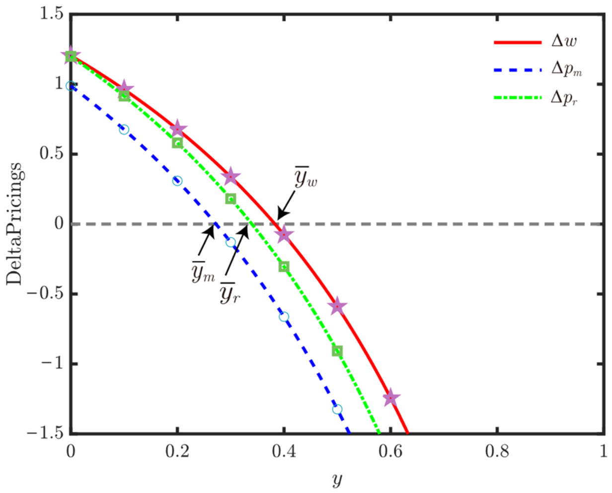
Let Δ w = w S O * w I O * , Δ p m = p m S O * p m I O * , Δ p r = p r S O * p r I O * , Φ = { Δ w , Δ p m , Δ p r } and κ = { y ¯ w , y ¯ m , y ¯ r } ; we have the following relationship: Φ > 0   if   0 < y < min { κ , 1 } < 0   if   max   κ < y < min { 16 τ 8 t 2 τ ρ 2 t 2 + 4 ρ t + 4 , 1 }
The core message of Proposition 3 is that pricing differences between the two channels are driven by bargaining ability rather than simple operating costs. Theoretically, this shows that the manufacturer’s pricing shifts from supporting the weak partner to protecting its own profit as the partner’s bargaining ability grows. Managerially, this means that bargaining ability is much more important than cutting internal costs. If a manufacturer does not manage the power structure first, a strong intermediary can easily wipe out any savings achieved through internal cost reductions.
Proposition 3 shows that the comparison depends entirely on the intermediary’s bargaining ability. When y is below the thresholds { y ¯ w , y ¯ m , y ¯ r } , all prices are higher in Model SO w S O * > w I O * , p m S O * > p m I O * , p r S O * > p r I O * ; see Figure 2. When y is above these thresholds, this relationship reverses. Specifically, when bargaining ability is low ( 0 < y < min { κ , 1 } ), the intermediary has little influence. To encourage the intermediary to participate, the manufacturer sets a lower wholesale price w I O and retail price p m I O , which also leads to a lower reselling price p r I O . In contrast, Model SO prices only reflect internal costs without bargain conflicts, making prices higher in Model SO than in Model IO. Conversely, when the intermediary’s bargaining ability is high ( max κ < y < min { 16 τ 8 t 2 τ ρ 2 t 2 + 4 ρ t + 4 , 1 } ), it will demand a high commission, cutting into the manufacturer’s profit. To recover this loss, the manufacturer raises w I O and p m I O , forcing the reseller to also raise p r I O . This makes all prices higher in Model IO than in Model SO. Ultimately, the price difference between the two models is driven by the bargaining ability.

4.2. Strategic Model Selections and Cooperation

Lemma 5. 
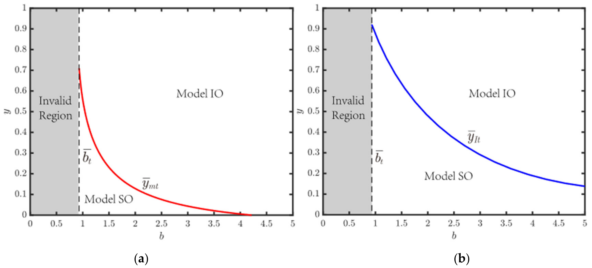
Comparing Model SO and Model IO, the manufacturer’s and intermediary’s optimal model selections are listed as follows. (i) When b > b ¯ t , π m I O * > π m S O * if y ¯ m t < y < 1 ; otherwise, π m S O * > π m I O * if 0 < y < y ¯ m t . (ii) When b > b ¯ t , π I I O * > π I S O * if y ¯ I t < y < 1 ; otherwise, π I S O * > π I I O * if 0 < y < y ¯ I t .
Lemma 5 shows that choosing between the two models depends on the trade-off between keeping a higher unit margin and achieving a larger sales volume. The core discovery is that neither channel is universally optimal, as preferences depend strictly on the intermediary’s bargaining ability. This misalignment happens because the manufacturer and intermediary operate under different bargaining ability thresholds ( y ¯ m t and y ¯ I t ). It means a channel structure can only succeed if it satisfies both parties’ profit requirements at the same time. Consequently, managers cannot make this decision based on internal costs alone. Instead, they must precisely evaluate the partner’s bargaining ability to locate the exact zone that will benefit both firms.
Lemma 5 (i) demonstrates that the manufacturer prefers Model IO only when bargaining ability exceeds the threshold y ¯ m t (see Figure 3a). In this region, the large sales scale driven by a powerful intermediary outweighs the loss from profit-sharing. When y < y ¯ m t , the manufacturer prefers Model SO because the intermediary’s limited reach cannot compensate for reduced unit margins. Similarly, Lemma 5 (ii) shows that the intermediary prefers Model IO only when the bargaining ability is above the threshold y ¯ I t to maximize its commission revenue (see Figure 3b). When y ¯ I t < y < 1 , the intermediary earns more from its baseline marketplace fees under Model SO and chooses to maintain the status quo.
Proposition 4. 
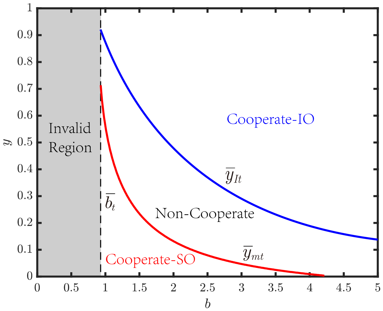
The feasible and non-feasible cooperation zones of Model SO and Model IO between the manufacturer and the intermediary are identified. (i) When b > b ¯ t , the manufacturer and the intermediary COOPERATE in Model IO if max { y ¯ m t , y ¯ I t } < y < 1 , and COOPERATE in Model SO if 0 < y < min { y ¯ m t , y ¯ I t } . However, the manufacturer and the intermediary DO NOT COOPERATE if max { y ¯ m t , y ¯ I t } < y < min { y ¯ m t , y ¯ I t } . (ii) y ¯ m t , y ¯ I t and b ¯ t increase in t , squeezing the profit margins of both Model SO and IO, notably making Model IO harder to survive.
Proposition 4 indicates that sustainable cooperation between firms only works when the intermediary’s bargaining ability is either very high or very low (See Figure 4). In the middle range, a mismatch in preferences creates a non-cooperation zone where partnerships naturally fail. To overcome this, the manufacturer should avoid a middle-ground intermediary entirely, or use contractual tools like tiered commissions and subsidies to artificially push the relationship into a cooperative zone. Furthermore, when market price competition t intensifies, it shrinks overall profitability and makes Model IO highly unviable. In highly competitive price wars, moving back to Model SO becomes an essential defensive move for the manufacturer to make to protect their remaining profit margins.
Particularly, when bargaining ability is high ( max { y ¯ m t , y ¯ I t } < y < 1 ), both firms agree on Model IO. The strong intermediary earns enough commission to cover its costs, while the manufacturer benefits from a huge sales volume that outweighs any profit-sharing losses. When bargaining ability is low ( 0 < y < min { y ˜ m , y ˜ I } ), both firms align on Model SO. Here, the weak intermediary prefers stable, low-risk marketplace returns, while the manufacturer finds self-live stream more profitable than sharing margins. However, an intermediate range ( max { y ¯ m t , y ¯ I t } < y < min { y ¯ m t , y ¯ I t } ), representing a mismatch such as y ¯ m t < y < y ¯ I t , creates a non-cooperation zone. In this middle area, one party’s optimal selection is the other’s worst choice, causing the outsourcing partnership to collapse.
Standard intuition and conventional wisdom might suggest that channel cooperation can be easily achieved under moderate bargaining ability. Under manufacturer leadership, cooperation favors moderate bargaining power (consistent with Chen et al. [24]). However, our formal game-theoretic derivation reveals the exact opposite, demonstrating that intuitive rules of thumb fail when channel leadership shifts. Rather than offering an incremental adjustment to Chen et al. [24], our study uncovers a fundamental strategic reversal: when the intermediary assumes Stackelberg leadership, moderate bargaining ability causes a complete collapse of cooperation, due to severe incentive misalignments. By explicitly modeling this leadership shift, our study establishes the analytical boundary conditions where traditional cooperation strategies break down. We show that when the intermediary acts as the leader and chooses the optimal model first, its profit-maximizing goal conflicts with the manufacturer’s. This conflict disappears under sole manufacturer leadership. By uncovering this non-trivial mechanics, our study explicitly establishes the analytical boundary conditions where traditional cooperation strategies break down under leadership transitions. Thus, our study provides new theoretical and managerial insights and subsequent strategies under this leadership change.
Proposition 4 (ii) shows that as cross-channel price competition t increases, the thresholds y ¯ m t , y ¯ I t and b ¯ t all shift upward. This happens because intense price competition hurts unit margins and cuts overall supply-chain profits. Under Model SO, the manufacturer keeps all unit profits, which provides stronger resilience against lower margins. Under Model IO, a shrinking profit margin must be split between two parties, meaning the model loses viability unless y is high enough to drive massive sales volume. As a result, fiercer price wars push the manufacturer further away from outsourcing and back toward self-operated live stream to protect their remaining profits.
In practice, as for intermediaries operating in highly competitive sectors, they should proactively lower their pit fees to align their incentives with the manufacturer’s sales-growth objectives, securing a more sustainable partnership. Meanwhile, platform operators should implement tiered platform service fees, specifically targeting highly competitive industries where dominant intermediaries are eager to extract predatory margins, distorting retail prices.

5. Extensions

5.1. Consumer Surplus and Social Welfare

This section investigates the implications of different live stream modes for consumer surplus (CS) and social welfare (SW). Beyond firm-level profitability, we examine how the interaction between the intermediary’s bargaining ability y and the cross-channel price competition intensity t reshapes market efficiency. We provide insights into how different live stream models influence stakeholder interests and overall market efficiency. The CS and SW functions for Model j { S O , I O } are defined as follows:
C S j = 0 q m j p m ( q m , q r j ) d q m + 0 q r j p r ( 0 , q r ) d q r ( p m j q m j + p r j q r j )
S W j = C S j + π m j + π r j + π I j
Proposition 5. 
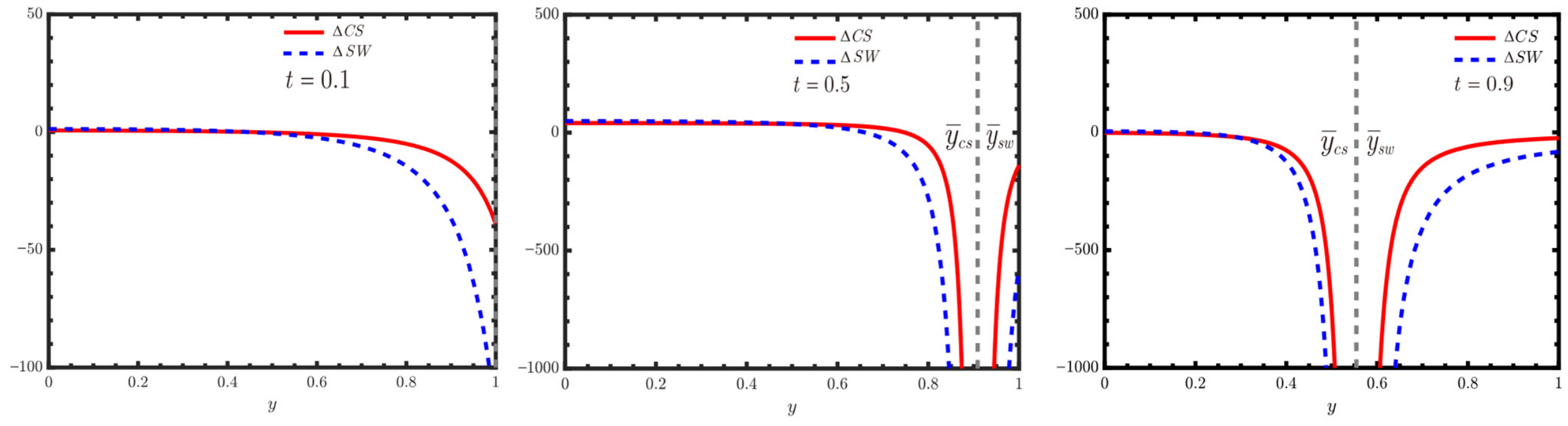
Define Δ C S = C S S O * C S I O * , Δ S W = S W S O * S W I O * ; we have the following relationships: (i) when t is low, Δ C S and Δ S W decrease in y ; (ii) when t is medium to high, Δ C S and Δ S W first decrease in y if 0 < y < min { y ¯ c s , y ¯ s w } , then increase in y if max { y ¯ c s , y ¯ s w } < y < 1 .
Proposition 5 provides clear guidance for managers and regulators, showing that market type changes how bargaining ability affects welfare. In low-competition sectors like high-end customization, the manufacturer should partner with top-tier intermediaries to reach new markets, and governments should encourage this growth. Conversely, in highly competitive markets like FMCG, dominant intermediaries can become welfare killers by triggering price hikes. Therefore, firms should choose moderately powerful partners instead of top-tier ones, while regulators should consider commission caps if social welfare begins to decline.
When cross-channel price competition t is low, the live stream and reselling channels do not fiercely compete. In this environment, a more powerful intermediary mainly drives market expansion. Even if prices rise slightly, the benefits of higher popularity, such as better consumer convenience, outweigh the negative impacts of higher prices. Consequently, both CS and SW increase steadily as y grows. However, when price competition is medium to high, a dual effect emerges. In the low- y stage ( 0 < y < min { y ¯ c s , y ¯ s w } ), initial gains from expanding popularity dominate, which boosts both CS and SW. But in the high- y stage ( max { y ¯ c s , y ¯ s w } < y < 1 ), a dominant intermediary demands high margins, forcing the manufacturer to raise prices across all channels (consistent with Lemma 3). This price hike triggers a sharp drop in consumer demand, causing both CS and SW to fall (see Figure 5). Under intense market competition, an overly powerful intermediary ultimately hurts both consumer and social welfare.

5.2. Negative Popularity Spillover Effect

In the base model, we assume a positive spillover synergy between the live stream and the reselling channel (i.e., 0 < ρ < 1 ). However, in practice, aggressive promotional tactics or brand mismatch may lead to brand dilution, where the influencer’s popularity negatively affects the traditional reselling channel. Well-known cases, such as conflicts between brands and top streamers, also suggest that spillover effects can be negative. We thus extend ρ to a negative range (i.e., 1 < ρ < 0 ) to discuss further influence.
Observation 1. 
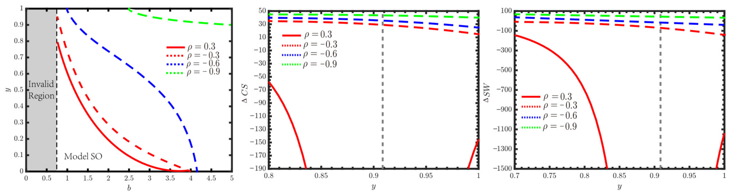
When ρ turns negative, it not only aggressively erodes the manufacturer’s strategic preference for Model IO at a faster rate, but also, counterintuitively, triggers a systemic collapse of CS and SW.
Observation 1 offers direct insights for all three parties. First, the manufacturer facing negative spillovers should prioritize Model SO to maintain stability. Second, the intermediary must focus on value-added services rather than aggressive profit-extraction to prevent the manufacturer from exiting. Finally, policy makers should actively limit dominant intermediaries by capping high commission rates and support brand-run channels to stop the shrinking of total social welfare.
Specifically, Observation 1 shows that Model IO suffers a rapid, nonlinear collapse when the spillover effect becomes negative (i.e., π m I O > π m S O ). The simulation’s results indicate that as ρ drops further below zero (from −0.3 to −0.6, and further to −0.9), the bargaining ability threshold required to sustain Model IO rises at an accelerating rate (see Figure 6). While ρ > 0 drives market expansion, a negative spillover triggers a severe cannibalization effect, where the live stream channel redirects demand from the manufacturer’s reselling channel. This strong encroachment shrinks the profitable zone for Model IO, forcing the manufacturer to switch to Model SO. Additionally, when ρ < 0 , a more powerful intermediary (i.e., higher y ) reduces both consumer surplus and social welfare. In this scenario, the intermediary’s influence creates severe internal friction rather than system efficiency, ultimately diminishing both CS and SW.

5.3. Consumer Channel Preference

Empirical evidence suggests that consumers often exhibit a distinct preference toward either traditional retail or live stream channels. To account for market heterogeneity, we thus introduce an exogenous parameter α [ 0 , 1 ) to represent the segment of consumers with a biased preference toward the reselling channel, while 1 α captures those with a predisposition for the live stream channel. The demand functions of both models in this extension are q r S O E = α p r S O E + t p m S O E + k T E and q m S O E = ( 1 α ) p m S O E + t p r S O E + T E for Model SO, and q r I O E = α p r I O E + t p m I O E + ρ L E and q m I O E = ( 1 α ) p m I O E + t p r I O E + L E for Model IO. Profit functions in this extension are the same as those in the base models. This extension allows us to explore how a diversified consumer base and the resulting channel competition influence the manufacturer’s mode selection.
Observation 2. 
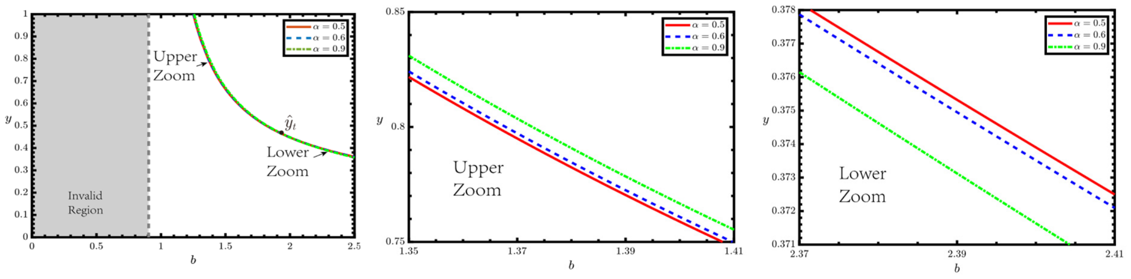
While α rises, the manufacturer preference toward Model IO decreases if y > y ^ t , otherwise preference toward Model IO increases if y < y ^ t .
Observation 2 shows that the decision to outsource in a shrinking market depends on balancing cooperation costs against channel efficiency. The threshold y ^ t represents this critical equilibrium. It marks the boundary where the intermediary’s popularity benefits exactly offset the manufacturer’s margin loss.
Particularly, Observation 2 shows that how an increasing preference for the reselling channel ( α ) affects the manufacturer’s channel selection depends heavily on the intermediary’s bargaining ability (see Figure 7). Specifically, under a powerful intermediary ( y > y ^ t ), an increase in α decreases the attractiveness of Model IO. As the live stream market ( 1 α ) contracts, the powerful intermediary’s high margin extraction creates a double squeeze. This pressure ultimately drives the manufacturer to choose Model SO to reclaim channel control. Conversely, under a weak intermediary ( y < y ^ t ), an increase in α increases the attractiveness of Model IO. Although the live stream segment is shrinking, a weak intermediary remains highly cost-effective. This partnership allows the manufacturer to maintain a channel presence without bearing operational burdens. Furthermore, the intermediary’s popularity acquisition easily offsets the minimal margin loss.

5.4. Popularity Cost Sharing Contract

The base model assumes the intermediary bears all popularity acquisition costs. However, in practice, manufacturers/brand owners often form strategic alliances with intermediaries to co-fund traffic acquisition. This extension introduces a popularity cost-sharing contract to reflect contemporary traffic subsidies. We introduce an exogenous parameter λ ( 0 , 1 ) to represent the popularity cost sharing ratio of the manufacturer. Therefore, the manufacturer bears λ τ L 2 / 2 y and the intermediary bears ( 1 λ ) τ L 2 / 2 y as to popularity acquisition costs. The demand functions and the rest of the profit functions of both models remain the same as those of the base model.
Proposition 6. 
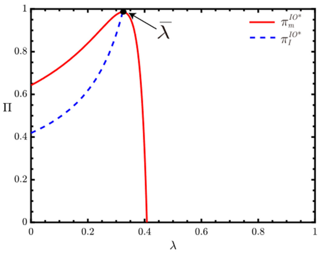
The profit of the manufacturer first increases in λ if 0 < λ < λ ¯ , then decreases in λ if λ ¯ < λ < 1 , while the increase in the profit of the intermediary in λ always holds.
Proposition 6 highlights the value of strategic coordination of cost-sharing between the two firms. Sharing popularity costs is highly beneficial because it aligns incentives and expands total supply-chain profits. However, the manufacturer must avoid over-subsidizing the intermediary. Intermediaries may try to actively co-invest in after-sales infrastructure or local operational support rather than demanding purely financial subsidies from the manufacturer. This shift from simple cash transfers to co-investment ensures a stable, win–win operational support structure.
Specifically, Proposition 6 shows that the cost-sharing ratio λ has divergent impacts on the profits of the manufacturer and the intermediary (see Figure 8). The manufacturer’s profit π m λ exhibits an inverted U-shaped relationship with λ . Specifically, it increases when 0 < λ < λ ¯ and decreases when λ ¯ < λ < 1 . In contrast, the intermediary’s profit π I 1 λ increases monotonically across the entire range of λ . This divergence stems from the trade-off between traffic stimulation and the cost burden. When λ is low ( 0 < λ < λ ¯ ), the manufacturer’s subsidy effectively motivates the intermediary to seek a higher popularity level. The resulting revenue growth outweighs the shared cost of λ τ L 2 / 2 y , leading to a Pareto improvement where both parties benefit. In this sense, our finding is in accordance with the study of He et al. [63], where the authors demonstrate that when the cost-sharing ratio of traffic investment is smaller, the brand owner is more willing to share the traffic cost, as she can obtain more profit. However, when λ exceeds the threshold, the marginal revenue from popularity diminishes. Meanwhile, the manufacturer’s share of the popularity investment cost grows too large. This heavy cost share outweighs the revenue gains, causing the manufacturer’s profit to decline while the intermediary’s profit continues to rise.

5.5. Manufacturer’s Live Stream Support

In Model IO, beyond delegating promotional tasks to the influencer, manufacturers in practice often provide operational support (e.g., product selection optimization, IT integration) to enhance live stream performance. We characterize this support as an endogenous fixed investment G with diminishing marginal returns η G in demand. η ( 0 , 1 ) represents the consumer sensitivity of this investment relative to increased demand. This extension aims to examine whether manufacturer-led support complements its own performance. For readability, specific model settings, the sequence of events and the equilibrium results are shown in the Appendix A.
Proposition 7. 
There exists a critical threshold of consumer sensitivity factor that influences the manufacturer’s optimal profit: π m I O G * η > 0   ( < 0 ) if η < η *   ( η > η * ) .
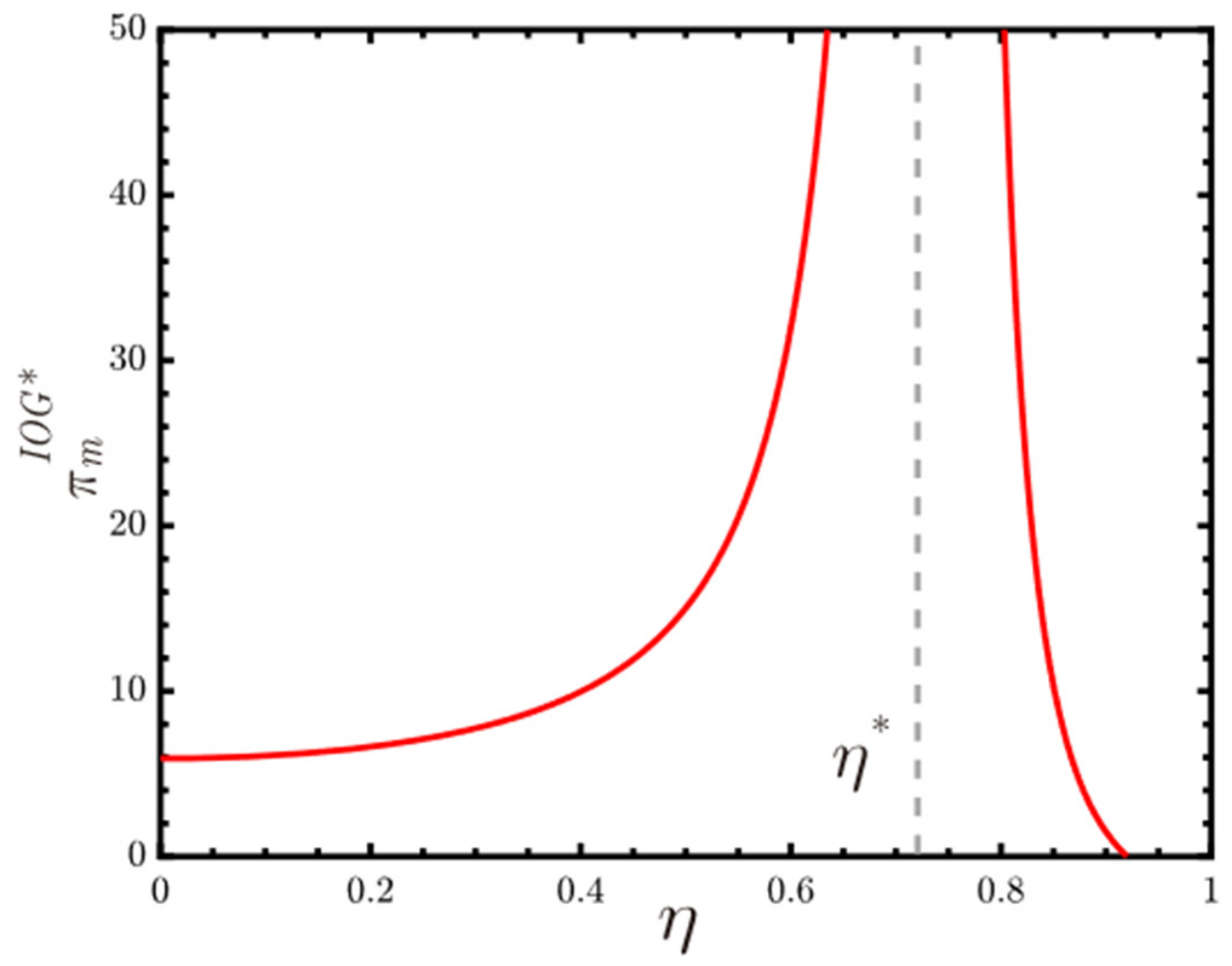
Proposition 7 highlights the risk of the over-service trap in customer service. While upgrading after-sales features can stimulate market demand, excessive support levels eventually erode profit margins. The threshold η * marks the critical tipping point for long-term channel strategy (see Figure 9). It defines the exact boundary where a manufacturer transitions from service-driven growth to service-eroded profit. Theoretically, this finding identifies a counter-intuitive paradox where sales expansion leads to profit decline.
Particularly, when consumer service sensitivity is low ( η < η *   ), an increase in η motivates the manufacturer to expand its support investment G * . This expansion successfully drives up both market demand and profit. However, when sensitivity crosses the threshold ( η > η * ), the hyper-sensitive market triggers a heavy over-investment in support. Although sales volume continues to rise, the escalating cost of providing these advanced services outweighs the revenue gains, causing the manufacturer’s profit to decline. In reality, such traps of over-services like “instant refunds,” “no-reason doorstep pickups,” or “full shipping insurance” are commonly seen.
In practice, to avoid this destructive trap, the manufacturer must resist blindly upgrading after-sales features to chase short-term sales volume. Furthermore, platform operators should design matchmaking and operational risk-sharing tools that help manufacturers assess market sensitivity thresholds, actively guiding firms away from unstable mid-tier partnerships and preventing competitive service escalation that harms overall channel welfare.

6. Conclusions

6.1. Concluding Remarks

Despite the rapid growth in dual-channel live stream supply chains, the existing literature lacks a systematic understanding of how intermediary bargaining ability, operational costs, and channel spillovers interact. This research gap leaves critical industry phenomena unexplained, such as counter-intuitive promotion investments, fluctuating commissions, and the risks of over-service. To bridge these gaps, this study constructs a game-theoretic framework comparing a manufacturer self-operated model (Model SO) with an intermediary-operated model (Model IO) to uncover the driving forces behind pricing and channel selection.
In Model SO, the live stream channel can serve as a traffic-channeling gateway to the traditional reselling channel. Surprisingly, rising live stream costs do not always reduce profits. Instead, higher costs can drive a strategic transformation toward this gateway role, which ultimately improves total efficiency. In Model IO, the impact of bargaining ability depends heavily on pit fees. High pit fees lead to predatory commissions. Conversely, low pit fees align incentives, turning the intermediary into a collaborative partner. Ultimately, bargaining ability acts as a double-edged sword that can either magnify revenues or escalate cost burdens. Critically, while the conventional wisdom assumes a monotonic relationship between this bargaining ability and profit extraction, our model proves that this mechanism is highly non-linear and moderated by distinct contract terms.
Comparing the two models reveals clear boundaries for sustainable cooperation. The manufacturer should generally avoid partnering with an intermediary who possess mid-tier bargaining ability, as incentive incompatibility prevents long-term alignment. Furthermore, intense cross-channel price competition reduces profits, directly threatening the sustainability of Model IO.
Finally, we extend the model to evaluate consumer surplus and social welfare. Negative spillover weakens the gateway role, forcing defensive pricing. However, high channel preference mitigates the margin squeeze from a powerful intermediary. We also find an optimal cost-sharing threshold for incentive alignment, and warn the manufacturer against an over-service trap that erodes profits. These results show that firms must balance operational support with power structures and spillover effects.

6.2. Theoretical and Managerial Implications

This study advances the theoretical landscape of dual-channel supply-chain management and live stream e-commerce across the following five dimensions. A primary theoretical contribution lies in separating intuitive, empirical expectations from model-derived, non-trivial analytical boundaries:
First, reconceptualization of channel roles. We challenge the view of channels as static profit centers by showing that the live stream channel can be repositioned as a traffic-channeling gateway. This reveals how low-margin channels can subsidize high-margin channels, extending multi-channel coordination theory.
Second, the multifaceted impacts of an intermediary’s bargaining ability. We show that bargaining ability is a double-edged sword performing both profit extraction and supply-chain coordination. The intermediary’s role as a predator or a partner is endogenously determined by the interaction of bargaining ability and pit fees. Furthermore, powerful intermediaries can act as “welfare killers” by distorting prices in highly competitive markets. This disrupts linear assumptions of power influence, offering theoretical support for antitrust regulations and commission caps.
Third, endogenous pricing and strategy transformation. We prove that cross-channel pricing differentials are driven by bargaining ability rather than operational costs alone. This provides a micro-theoretical foundation for pricing strategy evolution in live stream retailing.
Fourth, incentive alignment and governance boundaries. We define precise boundaries for switching between Model SO and Model IO based on bargaining ability ranges. Our framework identifies specific cooperation and non-cooperation zones, offering quantitative boundaries for transaction cost theory. Contrary to standard management intuition that expects smooth coordination under mid-tier bargaining ability, we explicitly prove that leadership shifts induce complete cooperation collapse in this intermediate range, highlighting the necessity of our formal analytical modeling.
Lastly, cost-sharing mechanism and over-service trap. We identify a Pareto-optimal threshold λ ¯ for cost-sharing contracts. Critically, we reveal an over-service trap when consumers are highly service-sensitive ( η > η * ), establishing a negative feedback boundary for service-driven growth theories.
This study offers the following key managerial insights for practitioners and regulators:
First, managers should adopt dynamic channel portfolio management and move beyond evaluating the live stream channel solely as a profit center. It also functions as a traffic-channeling gateway when channel cost is high but promotion cost is low. Taking advantage of channel spillover effects, manufacturers should actively increase promotion efforts, wholesale prices, and live stream retail prices to push consumers to the reselling channel. To facilitate this gateway mechanism, platform operators should offer targeted traffic-matching algorithms for high-cost manufacturers, while intermediaries should focus on optimizing cross-channel traffic redirection rather than demanding high direct sales margins.
Second, managers can strategically use low pit fees to align powerful intermediaries with sales-growth objectives and avoid bargaining ability weaponization. Furthermore, managers should start adaptive intermediary selection. In low-competition sectors, the manufacturer should embrace top-tier intermediaries to expand market reach. However, in high-competition markets, the manufacturer should favor moderate intermediaries to avoid the “welfare killer” effect of price distortions. As for intermediaries operating in highly competitive markets, they should proactively lower pit fees to secure long-term, sustainable partnerships. To maintain ecosystem health, platform operators should implement tiered platform service fees specifically targeting highly competitive industries where dominant intermediaries tend to extract predatory margins.
Third, when partnering with emerging intermediaries, the manufacturer should adopt a supportive pricing strategy to facilitate channel entry for these partners. However, as the intermediary’s influence grows, managers must be prepared to pivot to adjusting wholesale and retail prices to defend margins against commission extraction. Correspondingly, emerging intermediaries should accept lower commission rates in their early growth stage to build trust and secure stable volume guarantees from the manufacturer.
Fourth, while standard intuition might suggest seeking mid-tier intermediaries as a safe choice, our analytical results caution against this strategy, considering the different leadership structure. Since cooperation is most stable at the two extremes of the bargaining ability ranges, managers should avoid mid-bargaining-ability zones where incentive incompatibility occurs. Furthermore, firms should prioritize Model SO as a defensive measure when facing intense price competition. To minimize these cooperation failures, platform operators should design matchmaking and risk-sharing tools that actively guide manufacturers away from these unstable mid-tier partnerships.
Lastly, managers should implement popularity cost-sharing contracts but keep them strictly capped below the threshold ratio to avoid over-subsidizing the intermediary. Crucially, firms must resist service over-investment that increases sales volume but ultimately destroys profit through escalating operational costs. To avoid this trap, intermediaries may try to co-invest in after-sales infrastructure rather than demanding purely financial subsidies, ensuring a sustainable, win–win operational support structure.

6.3. Robustness, Limitations and Future Research

To ensure the academic rigor of our study, we first discuss the robustness of our analytical findings across several dimensions. First, our model assumptions and parameter settings strictly follow the stylistic approaches established in the leading operations management and marketing literature. Second, all our mathematical models are solved analytically, yielding closed-form equilibrium solutions that are mathematically rigorous and free from numerical approximation bias. Third, we perform extensive numerical analyses to validate the economic intuition and managerial implications of these analytical equilibria, ensuring their practical applicability under diverse market conditions. Crucially, our core insights, specifically the traffic-channeling gateway and the multifaceted impacts of bargaining ability, possess robust structural stability. Rather than being artifactual outcomes of specific parameters, these findings are driven by fundamental double-marginalization and spillover effects, and offer direct, robust theoretical contributions to strategic channel governance and sustainable cooperation.
Despite these robust insights, methodologically, our analytical framework relies on the assumption of complete information and fully rational decision-makers within a static game-theoretic setting. In reality, supply-chain members face information asymmetry, bounded rationality, and dynamic, multi-period interactions that may alter long-term cooperation stability. Additionally, while our stylized linear demand and cost structures ensure mathematical tractability, they inevitably simplify the highly non-linear nature of actual e-commerce operations. To address these limitations, future analytical models should incorporate asymmetric information and bounded rationality to examine how informational constraints alter channel dynamics. Moreover, developing multi-period, non-linear game models would help capture the dynamic evolution of cooperation stability in highly volatile digital markets.
To bridge the gap between our game-theoretic formulations and real-world operations, future studies should pursue empirical validation, which is highly relevant for digital commerce research. First, future empirical work could leverage consumer clickstream or search data to precisely measure the strength of cross-channel spillovers and quantify the actual conversion rate of the traffic-channeling gateway role identified in our Model SO. Second, researchers can utilize panel data or transaction-level data from live stream platforms to empirically test the over-service trap and the proposed U-shaped relationship between competitive intensity and cooperation inclination. Third, employing quasi-experimental methods, such as Difference-in-Differences (DiD) or Regression Discontinuity Designs (RDD), may help evaluate the empirical impact of regulatory policy shocks, such as government-imposed commission caps, on channel welfare and pricing distortions.

Author Contributions

Conceptualization, W.X.; methodology, W.X.; software, W.X.; validation, W.X.; formal analysis, W.X.; investigation, W.X.; writing—original draft preparation, W.X.; writing—review and editing, W.X. and X.S.; visualization, W.X.; supervision, X.S.; project administration, X.S.; funding acquisition, X.S. All authors have read and agreed to the published version of the manuscript.

Funding

This work was supported by the National Natural Science Foundation of China (NSFC) under Grant Nos. 72471183 and 71971165.

Institutional Review Board Statement

Not applicable.

Informed Consent Statement

Not applicable.

Data Availability Statement

The original contributions presented in this study are included in the article. Further inquiries can be directed to the corresponding author.

Conflicts of Interest

The authors declare no conflicts of interest.

Appendix A

Proof of Lemma A1. 
First, to ensure the equilibrium results are valid, we first verify the concavity of the profit functions. In the retail channel, 2 π m S O ( p r S O ) 2 = 2 < 0 . In the manufacturer’s live stream, 2 π m S O ( p m S O ) 2 = t 2 2 . Since 0 < t < 1 , the profit functions are strictly concave with respect to prices. Then, substituting the pricing response functions into π m S O ( w , T ) , we derive the Hessian Matrix H . For π m S O to be det ( H ) = k 2 t 2 + 4 b t 2 + k 2 + 4 k t 4 b + 2 2 ( 2 t 2 ) > 0 . Given 2 t 2 > 0 , this requires b > b = k 2 t 2 k 2 4 k t 2 4 t 2 4 . Under this condition, we calculate the FOCs π m S O w = 0 and π m S O T = 0 , yielding a unique optimal solution.
Second, we conduct sensitivity analysis of pricings on key parameters. We have the following results. (i) Impact of spillover intensity k . Differentiating w S O * and p r S O * with respect to k : w S O * k = N w ( b , c , k , t ) ( Δ S O ) 2 , p r S O * k = N p r ( b , c , k , t ) ( Δ S O ) 2 , where Δ S O = 2 ( k 2 t 2 + 4 b t 2 + k 2 + 4 k t 4 b + 2 )
N w = N p r = ( t 4 + t 2 2 ) k 2 + ( 8 b t 3 4 t 3 8 b t + 4 t ) k + ( 4 b t 4 + 4 b t 2 8 b 6 t 2 + 4 ) c ( t 3 + 2 t 2 + t 2 ) k 2 + ( 8 b t 2 16 b t 8 b + 4 t 2 + 4 t + 4 ) k + ( 4 b t 3 8 b t 2 12 b t 8 b + 6 t + 4 )
Setting N w , N p r = 0 yields critical values b , c 1 and c 2 . Under given b < b If c > max { c 1 , c 2 } , then w S O * k > 0 , p r S O * k > 0 ; otherwise, if c < max { c 1 , c 2 } , w S O * k < 0 , p r S O * k < 0 . For p m S O * with respect to k : p m S O * k = ( 4 t 2 4 ) ( k t 2 k t + 2 t 2 ) ( b b ) ( c c ) ( Δ S O ) 2 ; since 4 t 2 4 < 0 , the sign follows ( b b ) ( c c ) . (ii) Impact of cost coefficient b k . Differentiating optimal prices with respect to b : ( w S O * , p r S O * , p m S O * } b = ( t 2 1 ) ( ( c c ) ( k t 2 k t + 2 t 2 ) + k t + k + 2 ) * Γ ( Δ S O ) 2 , where Γ = 4 ( 1 t 2 ) ( k t + t + 2 ) is a positive, then the sign is determined by c c where c = k t k 2 k t 2 k t + 2 t 2 . If c > c , the manufacturer increases prices to compensate for the marginal loss in promotion efficiency. (iii) Impact of the live stream channel Fee c . Differentiating with respect to c , w S O * c = k 2 t + k t 2 + 2 k + 2 t Δ S O . The sign of this derivative depends on the denominator Δ S O . Through algebraic manipulation of b , we find that when b < b , the manufacturer maintains high efficiency and raises prices. In the range b < b < min { b 1 , b 2 } , the manufacturer strategically lowers prices to defend the retail channel against the rising c , while b > max { b 1 , b 2 } leads to standard cost-pass-through price increases. □
Proof of Lemma A2. 
First, to ensure the mathematical validity of the optimal promotion effort T , the second-order condition (SOC) with respect to T yields: 2 π m S O T 2 = k 2 t 2 + k 2 + 4 k t + 2 2 t 2 b ; since 0 < t < 1 , the denominator 2 t 2 > 0 . For π m S O to be strictly concave with respect to T , we require 2 π m S O T 2 < 0 , which is satisfied if and only if b > b = k 2 t 2 k 2 4 k t 2 4 t 2 4 . Under this unique condition, π m S O ( T ) is strictly concave, ensuring that the stationary point obtained from the FOC π m S O T = 0 is globally unique and optimal.
Second, (i) Impact of cost coefficient b . Let Δ S O = 2 ( k 2 t 2 + 4 b t 2 + k 2 + 4 k t 4 b + 2 ) ; the optimal effort is T * = U T Δ S O , where U T = 2 ( 1 t 2 ) ( k t + 2 ) ( c c ) . Applying the quotient rule with respect to b yields: T * b = 16 ( 1 t 2 ) 2 ( k t + 2 ) ( c c ) ( Δ S O ) 2 ; since ( 1 t 2 ) 2 > 0 , ( k t + 2 ) > 0 and ( S O ) 2 > 0 , the sign of T * b follows ( c c ) . That is, if b > b and c < c , then ( c c ) < 0 , we have T * b < 0 . Otherwise, when ( c c ) > 0 , we have T * b > 0 . (ii) Impact of the live stream channel cost c . Differentiating T * with respect to c yields: T * c = 2 ( 1 t 2 ) ( k t + 2 ) Δ S O ; since 0 < t < 1 , the numerator is strictly positive. The sign of T * c is determined entirely by Δ S O . That is if b > b and c < c , then Δ S O > 0 , we have T * c < 0 . Otherwise, when ( c c ) > 0 , then Δ S O < 0 , we have T * c > 0 . □
Proof of Proposition A1. 
(i) For the manufacturer. First, differentiating π m S O * with respect to k yields: π m S O * k = 8 ( 1 t 2 ) ( k t + 2 ) ( A k b + B k ) Δ S O , where A k = 2 ( 1 t 2 ) ( ( c 1 ) 2 t + 2 ( c + 1 ) ( t 1 ) + ( 2 t ) ) B k = ( c + 1 ) ( k 2 t 3 + 2 k 2 t 2 + k 2 t + 4 k t 2 + 4 k t + 4 t 2 + 4 t + 4 ) . Given 0 < t < 1 , c > 0 , and 0 < k < 1 , the component B k is strictly positive ( B k > 0 ). For A k , the quadratic form inside the brackets with respect to ( c 1 ) has a positive discriminant, rendering A k > 0 across the entire domain. Since A k > 0 and B k > 0 , the numerator is strictly positive under the operational condition b > b > 0 . Thus, π m S O * k > 0 is universally proved. Second, differentiating π m S O * with respect to b yields: π m S O * b = 2 ( 1 t 2 ) 2 ( k t + 2 ) 2 ( c c ) 2 ( Δ S O ) 2 . Because ( 1 t 2 ) 2 > 0 , ( k t + 2 ) > 0 and ( c c ) 2 > 0 , the main algebraic block is strictly positive. The leading negative sign dictates that π m S O * b < 0 holds true for all parameter values. Third, differentiating π m S O * with respect to c yields: π m S O * c = 2 ( 1 t 2 ) ( k t + 2 ) Ω Δ S O where Ω = ( 4 4 c + 2 t 4 t 2 + 6 c t 2 2 t 3 2 c t 4 ) b ( k k 2 + c k 2 + t k t + 2 c k t + c t 2 ) . Isolating b by setting Ω = 0 yields the structural threshold b 4 = k k 2 + c k 2 + t k t + 2 c k t + c t 2 4 + 4 c 2 t + 4 t 2 6 c t 2 + 2 t 3 + 2 c t 4 , which can be substituted back into the derivative to express Ω as a direct distance function: Ω = ( 4 + 4 c 2 t + 4 t 2 6 c t 2 + 2 t 3 + 2 c t 4 ) ( b b 4 ) . Recombining terms under the condition c > c , b < b 4 establishes that Ω > 0 , verifying π m S O * c > 0 . Symmetrically, rearranging Ω linearly with respect to c and setting Ω = 0 identifies the channel threshold c 3 = 2 b t 3 + 4 b t 2 2 b t + k 2 + k t 4 b k t 2 b t 4 6 b t 2 k 2 2 k t t 2 + 4 b . Transforming Ω into another form with respect to c 3 Ω = ( 2 b t 4 6 b t 2 k 2 2 k t t 2 + 4 b ) ( c 3 c ) . Therefore, under a stable system where unit promotion cost b > b and live stream channel fees are low c < c 3 , the evaluation shows Ω < 0 , verifying π m S O * c < 0 .
(ii) For the intermediary. First, applying the chain rule to differentiate π I S O * with respect to k yields the following formulation: π I S O * k = 16 ( 1 t 2 ) 2 ( k t + 2 ) ( c c ) ( 4 t 2 4 ) ( k t 2 k t + 2 t 2 ) ( b b ) ( c c ) ( Δ S O ) 3 ; since ( 4 t 2 4 ) < 0 , ( k t 2 k t + 2 t 2 ) = ( t 1 ) ( k t + 2 ) < 0 , their product is positive. The remaining sign of the derivative is driven by the interaction of the terms b b and c c against the cubed system denominator ( Δ S O ) 3 . If { c < c , b > b } , we have Δ S O > 0 , then ( Δ S O ) 3 > 0 . The evaluation yields a negative product inside the numerator which flips sign via the inner structural matrix transitions, confirming π I S O * k > 0 . If { c > c , b < b } , then ( Δ S O ) 3 < 0 , leading directly to π I S O * k < 0 . Second, differentiating π I S O * with respect to c produces the linear combination: π I S O * c = 8 ( t 2 1 ) ( k t 2 k t + 2 t 2 ) ( 2 b t 4 6 b t 2 k 2 2 k t t 2 + 4 b ) c + ( 2 b t 3 + 4 b t 2 2 b t + k 2 + k t 4 b k t ) ( Δ S O ) 3 . Setting the internal expression to zero isolates the unique inflection thresholds c 4 = 2 b t 3 + 4 b t 2 2 b t + k 2 + k t 4 b k t 2 b t 4 6 b t 2 k 2 2 k t t 2 + 4 and b 3 = k 2 + 2 k t + t 2 2 ( t 4 3 t 2 + 2 . Following similar logic, we derive the result that if { c > c 4 , b > b 3 } , the directional coefficients align positively with the denominator ( Δ S O ) 3 > 0 , meaning π I S O * c > 0 . If { c > c , b < b 3 } , the system parameters drop below the threshold requirements, creating a negative numerator shift, confirming π I S O * c < 0 . Third, differentiating π I S O * with respect to b produces the linear combination π I S O * b = c k t 2 + c + 1 k + 2 c t 2 c + k + 2 t + 1 2 t 1 c k t + 2 Δ S O . Following the same logic, if { c > c , b < b } , we have π I S O * b > 0 . Otherwise, while if { c < c , b > b } , we have π I S O * b < 0 . □
Proof of Lemma A3. 
The joint concavity of π I I O ( β , L ) requires the Hessian determinant to be strictly positive, defining the common denominator Δ I O for all equilibrium decisions, such as the following function: Δ I O = 2 ( 1 t 2 ) ( 8 τ ( 2 t 2 ) y ( ρ t + 2 ) 2 ) . Since 0 < t < 1 , a unique equilibrium exists if and only if τ > τ ^ = y ( ρ t + 2 ) 2 8 ( 2 t 2 ) .
(i) Impact of Intermediary’s Bargaining Ability y . Differentiating the pricing vector { w I O * , p m I O * , p r I O * } with respect to y via the quotient rule yields { w I O * , p m I O * , p r I O * } y = τ { Ω w y , Ω m y , Ω r y } ( Δ I O ) 2 . Substituting τ > τ ^ = y ( ρ t + 2 ) 2 8 ( 2 t 2 ) into the expanded polynomials shows that the numerators are strictly positive ( { Ω w y , Ω m y , Ω r y } > 0 ) across the stable domain. Thus, { w I O * , p m I O * , p r I O * } y > 0 always holds. (ii) Impact of spillover intensity ρ and unit pit fee δ . By setting the linear components of the partial derivatives to zero, we isolate the exact roots stated in Lemma 3. Differentiating with respect to ρ and solving for τ where the derivative equals zero yields the upper bound: τ 2 = ρ 2 t 2 y 4 ρ t y 4 y 8 t 2 16 = y ( ρ t + 2 ) 2 8 ( 2 t 2 ) . If τ > τ 2 , the strategic value of spillover dominates, ensuring { w I O * , p m I O * , p r I O * } ρ > 0 . By applying the quotient rule and grouping the numerator terms linearly relative to the thresholds, the derivatives are factored into the following explicit sign structures (where all denominators ( Δ I O ) 2 > 0 ). For the wholesale price, w I O * δ = 64 ( 1 t 2 ) ( 8 ρ + 8 t ) ( δ δ 1 ) ( Δ I O ) 2 , given τ < τ 1 ( τ τ 1 ) < 0 and δ < δ 1 ( δ δ 1 ) < 0 , it yields w I O * δ < 0 . For the live stream retail price, p m I O * δ = Φ m ( τ τ 3 ) ( δ δ 2 ) ( Δ I O ) 2 , where Φ m = 4 ( t 2 1 ) ( 12 ρ t 3 20 ρ t + 16 t 2 24 ) > 0 . Given the fact that τ < τ 3 ( τ τ 3 ) < 0 and δ < δ 2 ( δ δ 2 ) < 0 , their product is positive. The subgame pricing structure inverts this block, yielding p m I O * δ < 0 . For the reselling price, p r I O * δ = Φ r ( τ τ 4 ) ( δ δ 3 ) ( Δ I O ) 2 , where Φ r = 4 ( 2 ρ t 4 y 18 ρ t 2 y 12 t 3 y + 24 ρ y + 20 t y ) > 0 . Given the fact that τ < τ 4 ( τ τ 4 ) < 0 and δ < δ 3 ( δ δ 3 ) < 0 , the joint boundary forces p r I O * δ < 0 . □
Proof of Lemma A4. 
Applying the quotient rule to the optimal commission rate β * with respect to parameters y , ρ , and δ yields a strictly positive squared denominator: ( Δ 1 I O ) 2 > 0 , where Δ 1 I O = y ( ( ρ t + 2 ) 2 y + 8 t 2 τ 16 τ ) . The gradients are determined by the algebraic distance to the critical thresholds τ 5 and δ 4 .
First, sensitivity with respect to bargaining ability. Through algebraic isolation and double factoring, the numerator of β * y is structured as: β * y = 16 τ ( 4 t 2 8 ) ( τ τ 5 ) Ψ δ ( δ δ 4 ) ( Δ 1 I O ) 2 , where ( 4 t 2 8 ) < 0 for 0 < t < 1 . Case 1: When τ 2 < τ < τ 5 , the cost tension is absorbed by the channel structure, overriding the δ 4 threshold. Thus, ( τ τ 5 ) yields β * y > 0 . Case 2: When τ > τ 5 , the traffic acquisition cost is heavily prohibitive, shifting the sign control entirely to the pit fee distance vector ( δ δ 4 ) : if δ > δ 4 Ψ δ ( δ δ 4 ) < 0 , which mirrors the leading negative constant Ψ δ < 0 , proving β * y > 0 . Nevertheless, if δ < δ 4 Ψ δ ( δ δ 4 ) > 0 , aligning with the negative multiplier ( 4 t 2 8 ) < 0 , we have β * y < 0 . Second, sensitivities with respect to ρ and δ . Differentiating β * with respect to ρ and δ isolates the linear boundary δ 4 : β * ρ = 4 2 ρ 4 δ τ + y ρ 2 δ t 2 + 4 ρ + 1 τ + y ρ δ t + 8 2 δ + 1 τ + 4 δ y t ( Δ 1 I O ) 2 = M β ρ ( δ δ 4 ) ( Δ 1 I O ) 2 and β * δ = 4 ρ t y + 2 y Δ 1 I O , Under the equilibrium existence condition, τ > ρ 2 t 2 y 4 ρ t y 4 y 8 t 2 16   , we have Δ 1 I O < 0 .Therefore, β * δ = 4 ρ t y + 2 y Δ 1 I O > 0 always holds. Third, L * δ = y 8 ( t 2 2 ) Δ 1 I O > 0 always holds since ( t 2 2 ) < 0 and in the denominator, Δ 1 I O < 0 . L * y = 8 δ ( t 2 2 ) ( ρ t + 2 ) ( t + 2 ) Δ I O y 8 δ ( t 2 2 ) ( ρ t + 2 ) ( t + 2 ) ( ρ t + 2 ) 2 ( Δ 1 I O ) 2 . Let X 1 = 8 δ ( t 2 2 ) ( ρ t + 2 ) ( t + 2 ) < 0 , the numerator becomes X 1 [ Δ 1 I O y ( ρ t + 2 ) 2 ] , since Δ 1 I O y ( ρ t + 2 ) 2 = 8 τ ( t 2 2 ) < 0 and X 1 < 0 ; we thus have L * y > 0 , which always holds. Following the same logic, we have L * ρ = y t ( t + 2 ) Δ 1 I O y [ 8 δ ( t 2 2 ) ( ρ t + 2 ) ( t + 2 ) ] 2 y t ( ρ t + 2 ) ( Δ 1 I O ) 2   > 0 , which always holds since Δ 1 I O < 0 , X 1 = 8 δ ( t 2 2 ) ( ρ t + 2 ) ( t + 2 ) < 0 in the numerator. □
Proof of Proposition A2. 
To investigate the marginal impact of the intermediary’s bargaining ability on the optimal manufacturer profit π m I O * , we evaluate the first- and second-order derivatives with respect to y . By executing the quotient rule over the equilibrium profit function, the first-order condition satisfies
π m I O * y = N 1 ( y ) 4 Ω 2 ( t 2 1 )
where Ω = y ( ρ t + 2 ) 2 + 8 τ ( t 2 2 ) ,   N 1 ( y ) = A 1 y + A 0 .
A 1 = 12 τ ( t 2 2 ) 4 + ( ρ 8 δ ) t 2 + 2 ( ρ + 1 ) t + 16 δ ( δ ρ 2 t 4 + 4 δ ρ t 3 1 3 ( δ + 1 3 ) ρ 2 t 2 + 4 3 δ t 2 + 1 3 ( ρ 3 + ρ 2 28 δ ρ 2 ρ + 2 ) t 8 3 ( δ + 1 4 ) ρ 2 4 δ )  
A 0 = 12 τ ( t 2 2 ) 4 + ( ρ 8 δ ) t 2 + 2 ( ρ + 1 ) t + 16 δ ( 1 3 ( ρ + 16 δ ) τ t 4 + 2 3 ( ρ + 1 ) τ t 3 4 3 ( 12 δ + 1 ) τ t 2 10 3 ( ρ + 1 ) τ t + 32 3 ( δ 1 8 ) τ )
Based on the system’s Hessian stability conditions required for equilibrium existence, we strictly qualify Ω < 0 within the valid solution space.
H m = 2 π m w 2 2 π m w p m 2 π m p m w 2 π m p m 2
Since cross-price sensitivity satisfies 0 < t < 1 , we inherently have ( t 2 1 ) < 0 . Thus, the first-order denominator is globally negative. We then differentiate the FOC further with respect to y ; the second-order partial derivative can be mathematically structured into a quadratic rational format:
2 π m I O * y 2 = S 1 ( y ) ( t 2 1 ) Ω 4
where
S 1 ( y ) =   24 t 2 2 4 + ρ 8 δ t 2 + 2 ρ + 1 t + 16 δ ρ 2 4 δ τ + δ ρ 2 y + 1 2 ρ τ t 6 + 8 δ y + τ ρ 3 + 3 ρ 2 τ + 16 δ ρ τ t 5 + δ + 1 3 y ρ 4 + y 3 τ 2 ρ 3 + 2 2 16 y 3 3 τ δ + 5 τ 3 ρ 2 + 14 ρ τ 3 + 80 δ τ 3 t 4 + y ρ 5 3 + y ρ 4 3 + 40 3 δ y 2 y 11 3 τ ρ 3 + 2 y 25 τ 3 ρ 2 + 4 4 4 y 5 τ δ τ ρ 3 + 4 τ 3 t 3 + 2 y 1 4 δ 3 ρ 4 + y 2 τ ρ 3 + 4 17 y + 7 τ δ 3 11 τ 2 y ρ 2 + 2 y 11 τ ρ + 8 y 13 τ δ 3 4 τ t 2 + 4 8 3 δ y y 2 3 τ ρ 3 + y 10 τ 3 ρ 2 + 8 5 y τ δ 2 y 25 τ ρ 3 + 2 y 3 11 τ 3 t 32 δ + 1 4 y + 2 τ ρ 2 3 + 8 y 4 τ ρ 3 + 16 y + 2 τ δ 8 τ
Under the feasible parameter space bounded by the channel viability threshold ( δ < δ 5 ) and standard capacities ( 0 < t < 1 , 0 < ρ , 0 < y , 0 < τ ), expanding the multi-order symbolic blocks confirms that the numerator is strictly positive. Given that the denominator satisfies   ( t 2 1 ) Ω 4 < 0 , we strictly prove: 2 π m I O * y 2 < 0       y ( 0 , 1 ) . Thus, this guarantees that π m I O * is strictly concave with respect to y . This mathematical profile ensures that any interior root derived from π m I O * y = 0   constitutes a unique global maximum.
First, when τ < τ l o n g , setting the first-order derivative to zero ( π m I O * y = 0   ) isolates the unique linear root of N 1 ( y ) , yielding the exact analytical peak threshold y ^ :
y ^   =   64 τ + 96 t 2 τ 32 t 4 τ 20 8 ρ 2 36 ρ t + 12 t 2 5 ρ 2 t 2 + 20 ρ t 3 + 5 ρ 2 t 4
By virtue of the strict concavity established in the former section, we map that π m I O * y > 0   when y < y ^   (market volume expansion effect dominates) and reverses to π m I O * y < 0   when y > y ^   (margin extraction effect dominates). This mathematically validates the non-monotonic trajectory.
To prove the global robustness of the directional regimes independently of the pit fee ( δ > 0 ), we linearize the unified first-order numerator N 2 ( y ) with respect to N 2 ( y ) = δ Φ 1 ( y , τ , ρ , t ) + Φ 0 ( y , τ , ρ , t ) . By factoring the exact parametric interaction block, the linear slope coefficient Φ 1 is explicitly isolated as
Φ 1 ( y , τ , ρ , t ) = 12 ( t 2 2 ) π m I O ( t ) y ( ρ t + 2 ) 2 8 τ ( 2 t 2 )
where π m I O ( t ) = 4 + ( ρ 8 δ ) t 2 + 2 ( ρ + 1 ) t + 16 δ > 0 . Given that the cross-price sensitivity natively satisfies 0 < t < 1 , it follows that ( t 2 2 ) < 0 . Under case (i): When y > 16 τ 8 t 2 τ 4 + 4 ρ t + ρ 2 t 2 8 τ ( 2 t 2 ) ( ρ t + 2 ) 2 . Multiplying by ( t 2 2 ) strictly ensures that the slope Φ 1 < 0 . Concurrently, the intercept satisfies Φ 0 < 0 across the structural cost domain. Therefore, N 2 ( y ) < 0 holds strictly solid for all δ > 0 . Therefore, we have π m I O * y < 0     ( δ > 0 ) . Conversely, under the case (ii) when y < 16 τ 8 t 2 τ 4 + 4 ρ t + ρ 2 t 2 , the internal block flips sign, yielding an increasing trajectory where the slope satisfies Φ 1 > 0 . Within the interior viable channel boundaries ( δ < δ 5 ), this strategic positioning ensures that the volume stimulation effect persistently offsets the marginal friction, yielding π m I O * y > 0     ( δ > 0 ) .
Second, when τ > τ l o n g , the traffic-pulling inefficiency prevents the formation of an interior optimal power peak y ^ within the ( 0 , 1 ) domain. By substantiating τ > τ l o n g into the linearized first-order numerator   N 1 ( y ) = A 1 y + A 0 , the marginal variable coefficient vanishes or maintains a uniform directional slope, meaning the sign control of the gradient bypasses the inflection of y entirely. Consequently, the strategic alignment partitions into two steady zones universally governed by the fixed pit fee barrier δ 5 : if δ < δ 5 , π m I O * y > 0     ( y ( 0 , 1 ) )   and if δ > δ 5 , π m I O * y < 0     ( y ( 0 , 1 ) )   . □
Proof of Corollary A1. 
Differentiate the optimal manufacturer profit symmetrically. The symbolic cross-derivative is structured as:
2 π m I O * δ y = δ Λ 1 ( y , τ , ρ , t ) Λ 0 ( y , τ , ρ , t ) 4 Ω 3 ( t 2 1 )
where Λ 1 = t 6 H 6 + t 5 H 5 + t 4 H 4 + t 3 H 3 + t 2 H 2 + t H 1 + H 0
H 6 = 64 ρ 3 y 2 1280 δ ρ 2 y 2 8192 δ τ y + 256 ρ τ y H 5 = 128 ρ 3 y 2 5120 δ ρ y 2 + 384 ρ 2 y 2 + 512 ρ τ y + 512 τ y H 4 = 3840 δ ρ 2 y 2 64 ρ 3 y 2 + 1024 ρ 2 y 2 + 3072 τ y 3072 δ y 2 H 3 = 128 ρ 3 y 2 + 19456 δ ρ y 2 640 ρ 2 y 2 + 2048 ρ y 2 + 512 τ y H 2 = 40960 δ τ y 512 ρ 2 y 2 768 ρ τ y + 512 ρ y 2 65536 δ τ y 2 + 11264 δ y 2 768 ρ y 2 + 1024 y 2 H 1 = 512 ρ 2 y 2 + 2560 ρ τ y 512 ρ 3 y 2 768 ρ 2 y 2 3072 ρ τ y + 512 τ y + 40 $ $ H 0 = 32768 δ τ y 2 10240 δ y 2 4096 ρ τ y + 1024 ρ y 2 1024 y 2
Λ 0 = t 6 G 6 + t 5 G 5 + t 4 G 4 + t 3 G 3 + t 2 G 2 + t G 1 + G 0
G 6 = ρ 3 y + 2 ρ τ   G 5 = 2 ρ 3 y + 6 ρ 2 y + 4 ρ τ   G 4 = 16 ρ 2 y ρ 3 y 6 ρ τ + 8 ρ y + 24 τ   G 3 = 2 ρ 3 y 10 ρ 2 y + 4 τ + 4 ρ τ + 32 ρ y   G 2 = 8 ρ 2 y + 20 ρ τ 12 ρ 2 y + 16 y 56 τ   G 1 = 8 ρ 2 y 12 ρ y 24 ρ τ 40 ρ y 24 τ + 8 y   G 0 = 16 y 16 ρ 2 y 32 ρ τ + 16 ρ y + 16 τ
Based on the system’s Hessian stability conditions, the channel determinant satisfies Ω < 0 .
H = 2 ρ t + 2 ρ t + 2 8 τ + 4 y
Det ( H ) > 0 Ω = y ( ρ t + 2 ) 2 + 8 τ ( t 2 2 ) < 0
Since the cross-price sensitivity dictates 0 < t < 1 , we inherently have ( t 2 1 ) < 0 . Thus, the denominator is globally positive: 4 Ω 3 ( t 2 1 ) . By setting the linear numerator to zero, we isolate the unique inflection threshold for the pit fee: δ t h r e s = Λ 0 ( y , τ , ρ , t ) Λ 1 ( y , τ , ρ , t ) . Case (i): When δ > max { δ 4 , δ 6 } δ t h r e s = Λ 0 ( y , τ , ρ , t ) Λ 1 ( y , τ , ρ , t ) , the linear scaling ensures the numerator block is strictly positive, yielding 2 π m I O * δ y < 0 (cost-magnification effect). Case (ii): When δ < min { δ 4 , δ 6 } δ t h r e s = Λ 0 ( y , τ , ρ , t ) Λ 1 ( y , τ , ρ , t ) , the trajectory reverses, therefore yielding 2 π m I O * δ y > 0 (revenue-magnification effect). □
Proof of Proposition A3. 
Comparing the equilibrium pricing vectors under the SO Model and IO Model, the direct structural deviation vector is defined as Φ = { Δ w , Δ p m , Δ p r } . By introducing the common equilibrium scaling framework, the simultaneous comparison maps to a unified polynomial balance relation with respect to the platform’s capability parameter y . Δ w = w S O * w I O * = c k t 2 + c k 2 k 2 4 b + 2 c + k t + 2 c k 2 k 4 b + 2 2 k 2 + 8 b t 2 + 8 k t + 2 k 2 8 b + 4 + ρ 2 + 8 δ ρ t 2 + 8 δ + 2 ρ y + 8 τ t + 1 t 2 2 2 ρ 2 t 2 y + 4 ρ t y + 8 t 2 τ 16 τ + 4 y t 1 t + 1 yields y ¯ w , Δ p m = p m S O * p m I O * = 2 c k 2 + 2 b t 2 + 7 c k 4 b t + k 2 4 b + 4 c + k 2 k 4 b 2 k 2 + 8 b t 2 + 8 k t + 2 k 2 8 b + 4 + 12 δ ρ y + τ t 3 + ρ 2 + 16 δ + ρ y + 16 τ t 2 + 2 1 + 10 δ 1 ρ y 10 τ t 24 δ y 24 τ 2 t 1 ρ 2 y + 8 τ t 2 + 4 ρ t y + 4 y 16 τ t + 1 to derive y ¯ m .
Δ p r = p r S O * p r I O * = 2 b c t 3 + 2 c k + 2 b t 2 + 2 c 2 k 2 + 2 k + 2 c 4 b + 3 c t + 3 c 3 k 6 b + 3 2 k 2 + 8 b t 2 + 8 k t + 2 k 2 8 b + 4 + 2 δ ρ y 2 τ t 4 + 2 ρ 2 + 12 δ 2 ρ y + 12 τ t 3 + 4 + 18 δ + 4 ρ y + 18 τ t 2 + 3 ρ 2 20 δ + 3 ρ y 20 τ t + 6 + 24 δ 6 ρ y 24 τ 2 t 1 ρ 2 y + 8 τ t 2 + 4 ρ t y + 4 y 16 τ t + 1
to derive y ¯ r . By setting the functions to zero ( Δ w = 0 ), we isolate the unique, deterministic threshold for the bargaining ability. Since { w I O * , p m I O * , p r I O * } y > 0 , this means the higher the bargaining ability, the higher the pricings in Model IO. Therefore, it is easy to know that if 0 < y < min { κ , 1 } Δ w = w S O * w I O * > 0 , Δ p m = p m S O * p m I O * > 0 , Δ p r = p r S O * p r I O * > 0 . Otherwise, if κ < y < min { 16 τ 8 t 2 τ ρ 2 t 2 + 4 ρ t + 4 , 1 } , we obtain the opposite results. Specific bargaining ability thresholds ( κ = { y ¯ w , y ¯ m , y ¯ r } ) are shown in Table A1 at the end of the main text. □
Proof of Lemma A5. 
Following similar logic, we compare the equilibrium profits of the manufacturer and the intermediary under Model SO and Model IO respectively. We have Δ π m = π m S O * π m I O * , Δ π I = π I S O * π I I O * . By setting the functions to zero ( Δ π m = 0 , Δ π I = 0 ), we isolate the unique threshold for the bargaining ability, namely, y ¯ m t and y ¯ I t respectively, under the condition of b > b ¯ t = b , which makes equilibrium results positive. We have the following result.
Δ π m = π m S O * π m I O * = 2 c 2 t 3 + c 2 + 2 c t 2 + 2 c 2 + 2 c + 1 t + 2 c 2 4 c + 3 t + 1 b + c 1 k + c t + 1 2 16 t 2 16 b + 8 + 4 t 2 + 4 k 2 + 16 k t + ξ + ξ 1 4 t 1 ρ t + 2 2 y + 8 t 2 τ 16 τ 2 t + 1
where
ξ = 4 ρ 2 δ ρ 10 δ t 6 8 ρ δ ρ 2 20 δ + 3 ρ t 5 + ρ 4 + 4 δ + 2 ρ 3 + 120 δ 2 64 δ 1 ρ 2 32 ρ δ + 96 δ 2 t 4 8 δ + 1 2 ρ 2 + 5 δ 1 ρ + 76 δ 2 + 16 δ + 1 2 ρ t 3 + 2 ρ 4 4 ρ 3 + 16 δ 2 + 48 δ 2 ρ 2 + 48 δ + 8 ρ 352 δ 2 64 δ 4 t 2 + 32 δ + 8 ρ 3 + 32 δ 16 ρ 2 + 576 δ 2 + 160 δ + 8 ρ 32 δ t + 128 δ + 1 4 2 ρ 2 + 64 δ 16 ρ + 320 δ 2 + 64 δ + 8 y 2 ξ 1 = 16 δ ρ 16 δ t 3 + δ ρ + 16 δ + 2 t 2 + ρ 2 + 2 δ 1 ρ + 32 δ 2 + 10 δ t + 8 δ + 2 ρ 32 δ 2 4 δ 2 t + 1 τ t 2 2 y + 8 τ 2 t + 1 t 2 2 t 3 + 3 t 2 8 t 12
Δ π I = π I S O * π I I O * = c 2 t 2 2 c + t + 2 t 1 t + 1 b + k + t k + t c k + 1 8 t 2 8 b + 4 + 2 t 2 + 2 k 2 + 8 k t + 2 4 t 2 + 8 δ + t + 2 ρ t + 2 δ y + τ t + 2 2 2 ρ t + 2 2 y + 16 t 2 32 τ .
Specific threshold expressions of y ¯ m t and y ¯ I t are provided in Table A1 at the end of the main text. □
Proof of Proposition A4. 
It can be clearly observed that we consolidate the selection diagrams of the manufacturer and the intermediary for Model SO and Model IO in Lemma 5, based on which Proposition 4 (i) is derived. Due to incentive incompatibility, the manufacturer and the intermediary encounter conflicting intervals of their respective optimal profits in the medium range of y , which leads to the impossibility of cooperation. In Proposition 4 (ii), we test the sensitivity of these thresholds with respect to t. The results show that all three thresholds y ¯ m t , y ¯ I t and b ¯ t increase with t (i.e., b ¯ t = b = k 2 t 2 k 2 4 k t 2 4 t 2 4 , b ¯ t t = k + t k t + 1 t 2 1 2 > 0 ). This indicates that as price competition becomes more intense, the live stream profit margin gradually decreases, and Model IO exhibits the fastest declining rate. □
Proof of Proposition A5. 
Similarly, we adopt the same approach to compare consumer surplus (CS) and social welfare (SW) between Model SO and Model IO. We derive the corresponding equilibrium difference functions ( Δ C S = C S S O * C S I O * , Δ S W = S W S O * S W I O * ). By setting these functions equal to zero ( Δ C S = 0 , Δ S W = 0 ), we identify the unique thresholds of bargaining ability for Model SO and Model IO separately, namely, y ¯ c s and y ¯ s w . The explicit expressions of these specific thresholds are presented in Table A1 at the end of the main text.
C S S O * = 12 b 2 c 2 t 6 + 4 b c 2 k 2 t 4 + 4 b c 2 k t 5 40 b 2 c 2 t 4 + 24 b 2 c t 5 4 b c k 2 t 4 + 32 b 2 c t 4 12 b c 2 k 2 t 2 16 b c 2 k t 3 4 b c 2 t 4 + 4 b c k 2 t 3 + 8 b c k t 4 + 44 b 2 c 2 t 2 48 b 2 c t 3 + 12 b 2 t 4 + 20 b c k 2 t 2 + 12 b c k t 3 4 b k 2 t 3 c 2 k 4 4 c 2 k 3 t 5 c 2 k 2 t 2 2 c 2 k t 3 64 b 2 c t 2 + 32 b 2 t 3 + 8 b c 2 k 2 + 12 b c 2 k t + 4 b c 2 t 2 4 b c k 2 t 20 b c k t 2 8 b c t 3 8 b k 2 t 2 + 4 b k t 3 + 2 c k 4 + 6 c k 3 t + 4 c k 2 t 2 16 b 2 c 2 + 24 b 2 c t + 8 b 2 t 2 16 b c k 2 12 b c k t + 4 b k 2 t + 12 b k t 2 c 2 k 2 2 c 2 k t c 2 t 2 2 c k 3 6 c k 2 t 4 c k t 2 k 4 2 k 3 t + 32 b 2 c 32 b 2 t + 12 b c k + 8 b c t + 8 b k 2 4 b k t 4 b t 2 + 2 c k 2 + 2 c k t + 2 k 3 + 4 k 2 t 20 b 2 12 b k 2 c k 2 c t 2 k 2 2 k t + 4 b + 2 k 1 8 k 2 t 2 + 4 b t 2 + k 2 + 4 k t 4 b + 2 2
C S I O * = 12 δ 2 ρ 2 t 6 y 2 4 δ ρ 3 t 5 y 2 60 δ 2 ρ 2 t 4 y 2 + 16 δ 2 ρ t 5 y 2 + 4 δ ρ 2 t 5 y 2 + 24 δ ρ t 6 τ y + 4 δ ρ 3 t 3 y 2 16 δ ρ 2 t 4 y 2 + 16 δ ρ t 5 τ y 4 ρ 2 t 5 τ y + 48 δ 2 ρ 2 t 2 y 2 144 δ 2 ρ t 3 y 2 16 δ 2 t 4 y 2 4 δ ρ 2 t 3 y 2 120 δ ρ t 4 τ y + 16 δ ρ t 4 y 2 + 16 δ t 5 τ y + ρ 4 t 2 y 2 8 ρ 2 t 4 τ y + 4 ρ t 5 τ y + 12 t 6 τ 2 + 16 δ ρ 3 t y 2 + 32 δ ρ 2 t 2 y 2 144 δ ρ t 3 τ y 16 δ ρ t 3 y 2 32 δ t 4 τ y 2 ρ 3 t 2 y 2 + 4 ρ 2 t 3 τ y + 16 t 5 τ 2 + 64 δ 2 ρ 2 y 2 + 256 δ 2 ρ t y 2 + 16 δ 2 t 2 y 2 16 δ ρ 2 t y 2 + 96 δ ρ t 2 τ y 32 δ ρ t 2 y 2 144 δ t 3 τ y + 16 δ t 3 y 2 + 4 ρ 3 t y 2 + 24 ρ 2 t 2 τ y + ρ 2 t 2 y 2 20 ρ t 3 τ y 76 t 4 τ 2 + 8 t 4 τ y + 32 δ ρ 2 y 2 + 256 δ ρ t τ y + 48 δ ρ t y 2 + 32 δ t 2 τ y + 16 ρ 2 t τ y 8 ρ 2 t y 2 16 ρ t 2 τ y 144 t 3 τ 2 + 16 t 3 τ y + 64 δ 2 y 2 + 128 δ ρ τ y 32 δ ρ y 2 + 256 δ t τ y 48 δ t y 2 + 4 ρ 2 y 2 + 32 ρ t τ y + 4 ρ t y 2 + 64 t 2 τ 2 8 t 2 τ y + 128 δ τ y + 32 ρ τ y 8 ρ y 2 + 256 t τ 2 48 t τ y + 128 τ 2 32 τ y + 4 y 2 8 ρ 2 t 2 y + 4 ρ t y + 8 t 2 τ 16 τ + 4 y 2 t 2 1
S W S O * = 4 b c 2 k 2 t 6 + 12 b 2 c 2 t 6 4 b c 2 k 2 t 4 + 20 b c 2 k t 5 40 b 2 c 2 t 4 8 b 2 c t 5 4 b c k 2 t 4 32 b 2 c t 4 8 b c 2 k 2 t 2 48 b c 2 k t 3 + 12 b c 2 t 4 + 4 b c k 2 t 3 + 8 b c k t 4 4 b k 2 t 4 4 c k 4 t 2 4 c k 3 t 3 + 44 b 2 c 2 t 2 + 16 b 2 c t 3 20 b 2 t 4 12 b c k 2 t 2 20 b c k t 3 20 b k 2 t 3 c 2 k 4 4 c 2 k 3 t 5 c 2 k 2 t 2 2 c 2 k t 3 + 4 c k 3 t 2 + 4 c k 2 t 3 + 4 k 4 t 2 + 64 b 2 c t 2 96 b 2 t 3 + 8 b c 2 k 2 + 28 b c 2 k t 28 b c 2 t 2 4 b c k 2 t + 12 b c k t 2 + 24 b c t 3 12 b k t 3 2 c k 4 14 c k 3 t 12 c k 2 t 2 8 k 3 t 2 16 b 2 c 2 8 b 2 c t 56 b 2 t 2 + 16 b c k 2 + 20 b c k t 12 b k 2 t 100 b k t 2 c 2 k 2 2 c 2 k t c 2 t 2 + 2 c k 3 + 14 c k 2 t + 12 c k t 2 + 3 k 4 + 14 k 3 t + 4 k 2 t 2 32 b 2 c + 96 b 2 t + 16 b c 2 20 b c k 24 b c t 28 b k 2 52 b k t + 12 b t 2 6 c k 2 6 c k t 6 k 3 28 k 2 t + 76 b 2 + 36 b k 32 b t + 6 c k + 6 c t + 10 k 2 + 14 k t 44 b 14 k + 7 8 k 2 t 2 + 4 b t 2 + k 2 + 4 k t 4 b + 2 2
S W I O * = 52 δ 2 ρ 2 t 6 y 2 + 4 δ ρ 3 t 5 y 2 132 δ 2 ρ 2 t 4 y 2 + 240 δ 2 ρ t 5 y 2 + 256 δ 2 t 6 τ y 4 δ ρ 2 t 5 y 2 + 40 δ ρ t 6 τ y 4 ρ 4 t 4 y 2 + 4 ρ 2 t 6 τ y 68 δ ρ 3 t 3 y 2 48 δ ρ 2 t 4 y 2 + 112 δ ρ t 5 τ y + 8 ρ 3 t 4 y 2 + 20 ρ 2 t 5 τ y 176 δ 2 ρ 2 t 2 y 2 1136 δ 2 ρ t 3 y 2 1280 δ 2 t 4 τ y + 16 δ 2 t 4 y 2 + 68 δ ρ 2 t 3 y 2 72 δ ρ t 4 τ y + 48 δ ρ t 4 y 2 + 112 δ t 5 τ y + 7 ρ 4 t 2 y 2 16 ρ 3 t 3 y 2 44 ρ 2 t 4 τ y 4 ρ 2 t 4 y 2 + 12 ρ t 5 τ y + 52 t 6 τ 2 + 112 δ ρ 3 t y 2 32 δ ρ 2 t 2 y 2 752 δ ρ t 3 τ y 112 δ ρ t 3 y 2 224 δ t 4 τ y 14 ρ 3 t 2 y 2 84 ρ 2 t 3 τ y + 32 ρ 2 t 3 y 2 + 128 ρ t 4 τ y + 240 t 5 τ 2 + 448 δ 2 ρ 2 y 2 + 1280 δ 2 ρ t y 2 + 2048 δ 2 t 2 τ y 272 δ 2 t 2 y 2 112 δ ρ 2 t y 2 480 δ ρ t 2 τ y + 32 δ ρ t 2 y 2 752 δ t 3 τ y + 112 δ t 3 y 2 + 28 ρ 3 t y 2 + 88 ρ 2 t 2 τ y 9 ρ 2 t 2 y 2 + 4 ρ t 3 τ y 16 ρ t 3 y 2 116 t 4 τ 2 + 8 t 4 τ y + 224 δ ρ 2 y 2 + 1024 δ ρ t τ y + 208 δ ρ t y 2 + 224 δ t 2 τ y + 112 ρ 2 t τ y 56 ρ 2 t y 2 304 ρ t 2 τ y + 32 ρ t 2 y 2 1136 t 3 τ 2 + 176 t 3 τ y 1024 δ 2 τ y + 448 δ 2 y 2 + 896 δ ρ τ y 224 δ ρ y 2 + 1024 δ t τ y 208 δ t y 2 + 28 ρ 2 y 2 + 32 ρ t τ y + 28 ρ t y 2 448 t 2 τ 2 + 184 t 2 τ y 16 t 2 y 2 + 384 δ τ y + 224 ρ τ y 56 ρ y 2 + 1280 t τ 2 272 t τ y + 896 τ 2 288 τ y + 28 y 2 8 ρ 2 t 2 y + 4 ρ t y + 8 t 2 τ 16 τ + 4 y 2 t 2 1
Next, we conduct numerical analysis to examine how the threshold of y under different levels of price competition t affects Δ C S and Δ S W . The results show that no threshold of y exists when t is low ( t = 0.1 ), because both Δ C S and Δ S W always raise C S I O * and S W I O * . As t increases ( t = 0.5 , 0.9 ), C S I O * and S W I O * still rise when y is below the threshold ( y ¯ c s and y ¯ s w ). However, once y exceeds the threshold, C S I O * and S W I O * decrease substantially, implying that a higher bargaining ability erodes consumer surplus and social welfare in Model IO. □
Proof of Proposition A6. 
In this extension, we investigate the impact of a popularity cost sharing contract on both the manufacturer’s and the intermediary’s profits. We introduce an exogenous parameter λ ( 0 , 1 ) to represent the popularity cost sharing ratio of the manufacturer. Therefore, the manufacturer bears λ τ L 2 / 2 y and the intermediary bears ( 1 λ ) τ L 2 / 2 y as to popularity acquisition costs. We then extend our profit functions of Model IO to
max π m I O ( λ ) ( w I O , p m I O ) = w I O ( 1 p r I O + t p m I O + ρ L ) + ( p m I O y β ) ( 1 p m I O + t p r I O + L ) δ L λ τ L 2 2 y max π r I O ( p r I O ) = ( p r I O w I O ) ( 1 p r I O + t p m I O + ρ L ) max π I I O ( 1 λ ) ( β , L ) = y β ( 1 p m I O + t p r I O + L ) + δ L ( 1 λ ) τ L 2 2 y
We then obtain the following equilibrium results:
w I O ( λ ) = 4 δ ρ t 2 y + 8 δ ρ y 4 δ t 3 y + 8 δ t y + 4 λ t 3 τ + 4 λ t 2 τ 8 λ t τ 8 λ τ ρ 2 t 3 y 2 + ρ 2 t y + ρ t 3 y 2 ρ t 2 y ρ t y + 2 ρ y 4 t 3 τ 4 t 2 τ + t 2 y + 8 t τ + 8 τ 2 y t 2 1 8 λ t 2 τ + 16 λ τ + ρ 2 t 2 y + 4 ρ t y + 8 t 2 τ 16 τ + 4 y
p r I O = 2 δ ρ t 4 y 2 λ t 4 τ 2 ρ 2 t 3 y 18 δ ρ t 2 y 12 δ t 3 y + 12 λ t 3 τ + 2 ρ t 3 y + 2 t 4 τ + 18 λ t 2 τ + 3 ρ 2 t y 4 ρ t 2 y 12 t 3 τ + 24 δ ρ y + 20 δ t y 20 λ t τ 3 ρ t y 18 t 2 τ + 4 t 2 y 24 λ τ + 6 ρ y + 20 t τ + 24 τ 6 y 2 t 2 1 ρ 2 t 2 y + 8 λ t 2 τ 4 ρ t y 8 t 2 τ 16 λ τ + 16 τ 4 y
p m I O ( λ ) = 12 δ ρ t 3 y 12 λ t 3 τ ρ 2 t 2 y 20 δ ρ t y + 16 δ t 2 y 16 λ t 2 τ + ρ t 2 y + 12 t 3 τ + 20 λ t τ 2 ρ t y + 16 t 2 τ 24 δ y + 24 λ τ 20 t τ + 2 t y 24 τ 2 t 2 1 ρ 2 t 2 y + 8 λ t 2 τ 4 ρ t y 8 t 2 τ 16 λ τ + 16 τ 4 y
β ( 1 λ ) = 4 δ ρ t y λ t τ + 2 δ y 2 λ τ + t τ + 2 τ y ρ 2 t 2 y + 8 λ t 2 τ 4 ρ t y 8 t 2 τ 16 λ τ + 16 τ 4 y ,   L ( 1 λ ) = 8 δ t 2 ρ t 2 2 ρ t 16 δ 2 t 4 y ρ 2 t 2 y + 8 λ t 2 τ 4 ρ t y 8 t 2 τ 16 λ τ + 16 τ 4 y
q r I O = 2 δ ρ t 2 y 2 λ t 2 τ ρ 2 t y 8 δ ρ y 4 δ t y + 4 λ t τ + ρ t y + 2 t 2 τ + 8 λ τ 2 ρ y 4 t τ 8 τ + 2 y 2 ρ 2 t 2 y + 8 λ t 2 τ 4 ρ t y 8 t 2 τ 16 λ τ + 16 τ 4 y
q m I O ( λ ) = δ ρ t 3 y λ t 3 τ 2 δ ρ t y + 2 δ t 2 y 2 λ t 2 τ + t 3 τ + 2 λ t τ + 2 t 2 τ 4 δ y + 4 λ τ 2 t τ 4 τ ρ 2 t 2 y + 8 λ t 2 τ 4 ρ t y 8 t 2 τ 16 λ τ + 16 τ 4 y
π m I O ( λ ) = H 1 + H 2 + H 3 + H 4 4 ρ 2 t 2 y + 8 λ t 2 τ 4 ρ t y 8 t 2 τ 16 λ τ + 16 τ 4 y 2 t 2 1
π r I O = 2 δ ρ t 2 y 2 λ t 2 τ ρ 2 t y 8 δ ρ y 4 δ t y + 4 λ t τ + ρ t y + 2 t 2 τ + 8 λ τ 2 ρ y 4 t τ 8 τ + 2 y 2 4 ρ 2 t 2 y + 8 λ t 2 τ 4 ρ t y 8 t 2 τ 16 λ τ + 16 τ 4 y 2
π I I O ( 1 λ ) = 8 δ 2 t 2 y 2 δ ρ t 2 y 4 δ ρ t y + λ t 2 τ 16 δ 2 y 4 δ t y + 4 λ t τ t 2 τ 8 δ y + 4 λ τ 4 t τ 4 τ 2 ρ 2 t 2 y + 8 λ t 2 τ 4 ρ t y 8 t 2 τ 16 λ τ + 16 τ 4 y
H 1 = 40 δ 2 ρ 2 t 6 y 2 + 4 δ ρ 3 t 6 y 2 + 128 δ 2 λ t 6 τ y + 16 δ λ ρ t 6 τ y + 8 δ ρ 3 t 5 y 2 2 λ ρ 2 t 6 τ y + 120 δ 2 ρ 2 t 4 y 2 160 δ 2 ρ t 5 y 2 256 δ 2 t 6 τ y + 32 δ λ ρ t 5 τ y 4 δ ρ 3 t 4 y 2 + 24 δ ρ 2 t 5 y 2 + 16 δ ρ t 6 τ y 8 λ 2 t 6 τ 2 8 λ ρ 2 t 5 τ y + ρ 4 t 4 y 2 640 δ 2 λ t 4 τ y 48 δ λ ρ t 4 τ y + 32 δ λ t 5 τ y + 8 δ ρ 3 t 3 y 2 + 64 δ ρ 2 t 4 y 2 + 32 δ ρ t 5 τ y 32 λ 2 t 5 τ 2 22 λ ρ 2 t 4 τ y 8 λ ρ t 5 τ y H 2 = 16 λ t 6 τ 2 2 ρ 3 t 4 y 2 16 δ 2 ρ 2 t 2 y 2 + 608 δ 2 ρ t 3 y 2 + 1280 δ 2 t 4 τ y 96 δ 2 t 4 y 2 224 δ λ ρ t 3 τ y 64 δ λ t 4 τ y 40 δ ρ 2 t 3 y 2 48 δ ρ t 4 τ y + 32 δ ρ t 4 y 2 + 32 δ t 5 τ y + 56 λ 2 t 4 τ 2 8 λ ρ 2 t 3 τ y 16 λ ρ t 4 τ y + 64 λ t 5 τ 2 2 ρ 4 t 2 y 2 + 4 ρ 3 t 3 y 2 + 16 ρ 2 t 4 τ y + ρ 2 t 4 y 2 8 t 6 τ 2 + 1024 δ 2 λ t 2 τ y 96 δ λ ρ t 2 τ y 224 δ λ t 3 τ y 32 δ ρ 3 t y 2 48 δ ρ 2 t 2 y 2 + 32 δ ρ t 3 τ y + 128 δ ρ t 3 y 2 + 192 δ t 4 τ y + 224 λ 2 t 3 τ 2 + 40 λ ρ 2 t 2 τ y 40 λ ρ t 3 τ y 112 λ t 4 τ 2 8 λ t 4 τ y + 4 ρ 3 t 2 y 2 + 16 ρ 2 t 3 τ y 8 ρ 2 t 3 y 2 16 ρ t 4 τ y 32 t 5 τ 2 128 δ 2 ρ 2 y 2 576 δ 2 ρ t y 2 2048 δ 2 t 2 τ y + 352 δ 2 t 2 y 2 + 320 δ λ ρ t τ y H 3 = 64 δ λ t 2 τ y + 32 δ ρ 2 t y 2 + 160 δ ρ t 2 τ y 48 δ ρ t 2 y 2 + 32 δ t 3 τ y + 16 λ 2 t 2 τ 2 + 32 λ ρ 2 t τ y 32 λ ρ t 2 τ y 448 λ t 3 τ 2 8 ρ 3 t y 2 32 ρ 2 t 2 τ y + 2 ρ 2 t 2 y 2 + 16 ρ t 3 τ y + 4 ρ t 3 y 2 + 56 t 4 τ 2 512 δ 2 λ τ y + 256 δ λ ρ τ y + 320 δ λ t τ y 64 δ ρ 2 y 2 192 δ ρ t τ y 160 δ ρ t y 2 448 δ t 2 τ y + 64 δ t 2 y 2 320 λ 2 t τ 2 + 64 λ ρ t τ y 32 λ t 2 τ 2 + 8 λ t 2 τ y 32 ρ 2 t τ y + 16 ρ 2 t y 2 + 64 ρ t 2 τ y 8 ρ t 2 y 2 H 4 = 224 t 3 τ 2 32 t 3 τ y + 1024 δ 2 τ y 320 δ 2 y 2 + 128 δ λ τ y 256 δ ρ τ y + 64 δ ρ y 2 192 δ t τ y + 32 δ t y 2 192 λ 2 τ 2 + 64 λ ρ τ y + 640 λ t τ 2 32 λ t τ y 8 ρ 2 y 2 32 ρ t τ y 8 ρ t y 2 + 16 t 2 τ 2 32 t 2 τ y + 4 t 2 y 2 + 128 δ τ y 64 δ y 2 + 384 λ τ 2 32 λ τ y 64 ρ τ y + 16 ρ y 2 320 t τ 2 + 64 t τ y 192 τ 2 + 64 τ y 8 y 2
We now conduct a sensitivity analysis of the manufacturer’s profit and the intermediary’s profit with respect to λ . There exists a threshold of λ ¯ . When 0 < λ < λ ¯ , the relevant relationship holds ( π I I O ( 1 λ ) λ = H 1 + H 2 + H 3 + H 4 4 ρ 2 t 2 y + 8 λ t 2 τ 4 ρ t y 8 t 2 τ 16 λ τ + 16 τ 4 y 2 t 2 1 λ > 0 ). However, when λ ¯ < λ < 1 , the relationship changes accordingly ( π I I O ( 1 λ ) λ = H 1 + H 2 + H 3 + H 4 4 ρ 2 t 2 y + 8 λ t 2 τ 4 ρ t y 8 t 2 τ 16 λ τ + 16 τ 4 y 2 t 2 1 λ < 0 ). Given 0 < τ , 0 < y , the intermediary’s profit clearly increases monotonically with λ ( π I I O ( 1 λ ) λ = τ 4 + ρ 8 δ t 2 + 2 1 + ρ t + 16 δ 2 y 2 y ρ 2 8 τ λ 1 t 2 + 4 ρ t y + 16 τ λ 1 + 4 y 2 > 0 ). It is clear to see that the profit of the intermediary is monotonously increasing in λ . We adopt numerical analysis to verify this result, and the graphical illustration in Figure 8 is consistent with our theoretical expectation. □
Proof of Proposition A7. 
In this extension, we consider that the manufacturer provides live stream support to the intermediary and invests an endogenous service effort G . This effort positively influences the demand of live stream consumers and thereby increases market demand ( η G ). We extend the demand functions and profit functions as follows.
q r I O = 1 p r I O + t p m I O + ρ L q m I O = 1 p m I O + t p r I O + L + η G
max π m I O G ( w I O , p m I O , G ) = w I O ( 1 p r I O + t p m I O + ρ L ) + ( p m I O y β ) ( 1 p m I O + t p r I O + L + η G ) δ L G max π r I O ( p r I O ) = ( p r I O w I O ) ( 1 p r I O + t p m I O + ρ L ) max π I I O ( β , L ) = y β ( 1 p m I O + t p r I O + L + η G ) + δ L τ L 2 2 y
To investigate the strategic impact of the consumer sensitivity factor η on the manufacturer’s maximized operational profit π m I O G , we invoke the multi-stage backward induction tracking framework. According to the first-order conditions (FOCs) of the lower-stage pricing and traffic equilibrium, the optimal traffic attraction effort G * satisfies the unique market clearing property. The total derivative of π m I O G * with respect to η bypassing the indirect pricing variations can be condensed into: π m I O G * η = ( p m I O * y β * ) G * . Taking the second-order partial derivative of the value functions with respect to the consumer sensitivity matrix yields 2 π m I O G * η 2 = ( p m I O * y β * ) η G * + p m I O * y β * 2 G * G * η . By executing implicit differentiation on the foundational game structural equations system, we have ( p m I O * y β * ) η < 0 and G * η > 0 . Since the local marginal return of streaming pricing is bounded, the aggregate interaction matrix guarantees 2 π m I O G * η 2 < 0 . This strictly proves that the manufacturer’s optimal profit π m I O G * is strictly concave with respect to the consumer sensitivity factor η .
Given the definitive global concavity 2 π m I O G * η 2 < 0 , the optimization trajectory possesses at most a unique local turning point in the positive metric space. We set the FOC to zero: F ( η ) = π m I O G * η ( p m I O * y β * ) G * = 0 . Since the live stream attraction effort is strictly positive ( G * > 0 ) within the market-clearing boundary, the optimization zero-point collapses to the interior profit-margin balance: p m I O * ( η ) y β * ( η ) = 0 . When η 0 , the marginal benefit of direct volume pulls scales cleanly, leading to ( p m I O * y β * ) > 0 , hence F ( η ) > 0 . When η , the hyper-competition over traffic escalation erodes the pricing margin premium, forcing ( p m I O * y β * ) < 0 , hence F ( η ) < 0 . Therefore, there exists a unique, deterministic structural intersection root, denoted as η * , such that F ( η * ) = 0 .
Lastly, synthesizing the initial boundary signals and the system concavity tracking loops, the definitive segmented properties of Proposition 7 are formalized as follows. Case (i): When 0 < η < η *   , the system is bounded in the ascending stage where π m I O G * η > 0 . In this regime, the platform’s traffic expansion effect dominates, and an increase in η enhances the manufacturer’s profit. Case (ii): When η > η *   , the gradient crosses into the negative half-space where π m I O G * η < 0 . In this regime, the escalating burden of matching the service effort G heavily outpaces the revenue generation, creating an over-marketing trap that damages the manufacturer’s optimal profit. □
Table A1. Summary of other long thresholds used.
Long Thresholds
δ 6 3 y ρ 3 + 8 ρ τ t 6 + 6 y ρ 3 + 18 ρ 2 y + 16 ρ τ + 16 τ t 5 + 3 y ρ 3 + 44 ρ 2 y + 20 y 24 τ ρ + 96 τ t 4 + 2 y ρ 3 42 ρ 2 y + 72 y + 16 τ ρ 8 y + 16 τ t 3 + 8 y ρ 3 68 ρ 2 y + 68 y + 80 τ ρ + 16 y 224 τ t 2 + 32 y ρ 3 + 168 y 96 τ ρ + 8 y 96 τ t 64 ρ 2 y + 32 y 128 τ ρ 48 y + 64 τ 48 ρ 2 y + 16 τ 3 t 4 + 4 ρ t 3 y + ρ 2 y + 4 3 y 16 τ t 2 28 ρ t y 3 8 ρ 2 y 3 4 y + 32 τ 3 t 2 2
y ¯ w 8 τ ( c k t 6 c k 2 t 5 + c k t 4 + 3 c k 2 t 3 2 c t 5 k t 5 k 2 t 4 2 k t 4 2 k 2 t 3 2 c k 2 t + 4 c k t 2 + 6 c t 3 + k 2 t 2 k t 3 2 t 4 + 4 k 2 t + 2 k t 2 2 t 3 4 c k 4 c t + 2 k 2 + 6 k t + 4 t 2 + 4 k + 4 t ) N + P 1 + P 2 + P 3
y ¯ m 4 τ Q R
y ¯ r 2 τ S E 1 + E 2 + E 3
y ¯ m t 2 b c 2 t 4 6 b c 2 t 2 + 4 b c t 3 + 8 b c t 2 c 2 k 2 2 c 2 k t c 2 t 2 + 4 b c 2 4 b c t + 2 b t 2 + 2 c k 2 + 2 c k t 8 b c + 8 b t 2 c k 2 c t k 2 + 6 b + 2 k 1 4 ( k 2 t 2 + 4 b t 2 + k 2 + 4 k t 4 b + 2 ) + C 1 + C 2 4 ρ 2 t 2 y + 4 ρ t y + 8 t 2 τ 16 τ + 4 y 2 t 2 1 = 0
y ¯ I t c 2 b c t 4 6 b c t 2 + 2 b t 3 + 4 b t 2 c k 2 2 c k t c t 2 + 4 b c 2 b t + k 2 + k t 4 b k t 2 k 2 t 2 + 4 b t 2 + k 2 + 4 k t 4 b + 2 8 δ 2 t 2 y 2 δ ρ t 2 y 4 δ ρ t y 16 δ 2 y 4 δ t y t 2 τ 8 δ y 4 t τ 4 τ 2 ρ 2 t 2 y + 4 ρ t y + 8 t 2 τ 16 τ + 4 y = 0
y ¯ c s ( K 1 + K 2 + K 3 + K 4 ) 8 k 2 t 2 + 4 b t 2 + k 2 + 4 k t 4 b + 2 2 + ( O 1 + O 2 + O 3 + O 4 ) 8 ρ 2 t 2 y + 4 ρ t y + 8 t 2 τ 16 τ + 4 y 2 t 2 1 = 0
y ¯ s w M 1 + M 2 + M 3 + M 4 8 k 2 t 2 + 4 b t 2 + k 2 + 4 k t 4 b + 2 2 + N 1 + N 2 + N 3 + N 4 + N 5 8 ρ 2 t 2 y + 4 ρ t y + 8 t 2 τ 16 τ + 4 y 2 t 2 1 = 0
y ^ t A 1 + A 2 4 ( k 2 t 2 + 4 b t 2 + k 2 + 4 k t 4 b + 2 ) A 3 + A 4 + A 5 + A 6 4 ρ 2 t 2 y + 4 ρ t y + 8 t 2 τ 16 τ + 4 y 2 t 2 1 = 0
τ l o n g 16 δ 2 t 3 + δ ρ t 3 + 16 δ 2 t 2 + δ ρ t 2 + 32 δ 2 t 2 δ ρ t + 2 δ t 2 + ρ 2 t 32 δ 2 + 8 δ ρ + 10 δ t ρ t 4 δ + 2 ρ 2 t 3 + 3 t 2 8 t 12 2 ( Y 1 + Y 2 + Y 3 + Y 4 ) 4 t 3 + t 2 2 t 2 t 3 + 3 t 2 8 t 12 2
λ ¯ i = 1 9 B i 8 t 6 + 4 t 5 7 t 4 28 t 3 2 t 2 + 40 t + 24 τ
η *   π m I O G = w I O ( 1 p r I O + t p m I O + ρ L ) + ( p m I O y β ) ( 1 p m I O + t p r I O + L + η G ) δ L G , compute π m I O G * η to derive η *  
Note: Some of the threshold expressions are too long to be displayed properly in this table. Thus, we show the computation process to obtain the threshold. Detailed expressions are shown in the Appendix A.
P 1 = 4 c k t 4 + 4 c k ρ t 3 2 c k ρ 2 t 2 + 4 c k 2 t 3 4 c k 2 ρ t 2 + 8 c ρ t 4 2 c ρ 2 t 3 + 32 δ k t 4 + 32 δ k ρ t 3 8 δ k 2 t 3 8 δ k 2 ρ t 2 + 2 ρ 2 t 4 k ρ 2 t 3 + k 2 ρ t 3 2 k 2 t 4 96 b δ t 3 96 b δ ρ t 2 8 b t 4 4 b ρ t 3 + 4 b ρ 2 t 2 P 2 = 2 k 2 ρ 2 t + 2 k 2 ρ t 2 4 k 2 t 3 6 k ρ 2 t 2 + 2 ρ 2 t 3 + 8 b ρ 2 t 8 b ρ t 2 16 b t 3 4 c k 2 t 8 c k ρ t + 4 c k t 2 8 c ρ t 2 + 8 c t 3 16 δ k 2 ρ 16 δ k 2 t 64 δ k ρ t 64 δ k t 2 + 16 δ ρ t 2 + 16 δ t 3 + 2 k 2 ρ t + 2 k 2 t 2 P 3 = 4 k ρ t 2 4 k t 3 2 ρ 2 t 2 + 6 ρ t 3 + 64 b δ ρ + 64 b δ t + 8 b ρ t + 8 b t 2 4 k 2 ρ + 4 k 2 t 8 k ρ t 8 k t 2 4 ρ 2 t + 4 ρ t 2 + 16 b ρ + 16 b t 8 c k 8 c t 32 δ ρ 32 δ t + 4 k 2 + 12 k t 4 ρ t + 4 t 2 + 8 k 8 ρ
Q = 4 c k 2 t 6 8 b c t 6 + 10 c k 2 t 4 14 c k t 5 3 k 2 t 5 + 32 b c t 4 4 b t 5 6 k 2 t 4 8 b t 4 2 c k 2 t 2 + 42 c k t 3 8 c t 4 + 2 k 2 t 3 10 k t 4 40 b c t 2 + 8 b t 3 + 8 k 2 t 2 16 k t 3 + 16 b t 2 4 c k 2 28 c k t + 24 c t 2 + 5 k 2 t + 14 k t 2 6 t 3 + 16 b c 4 b t + 2 k 2 + 24 k t 8 t 2 8 b 16 c + 4 k + 10 t + 12
R = 2 c k 2 ρ 2 t 6 + 4 b c ρ 2 t 6 c k 2 ρ 2 t 4 + 8 c k 2 ρ t 5 + 7 c k ρ 2 t 5 + 12 δ k 2 ρ t 5 8 b c ρ 2 t 4 + 16 b c ρ t 5 + 48 b δ ρ t 5 4 b ρ 2 t 5 8 b ρ 2 t 4 c k 2 ρ 2 t 2 4 c k 2 ρ t 3 + 8 c k 2 t 4 7 c k ρ 2 t 3 + 28 c k ρ t 4 + 4 c ρ 2 t 4 8 δ k 2 ρ t 3 + 16 δ k 2 t 4 + 48 δ k ρ t 4 + k 2 ρ t 4 k ρ 2 t 4 + 4 b c ρ 2 t 2 32 b c ρ t 3 + 16 b c t 4 128 b δ ρ t 3 + 64 b δ t 4 + 4 b ρ 2 t 3 12 b ρ t 4 2 k 2 ρ 2 t 2 + 2 k 2 ρ t 3 4 k ρ 2 t 3 + 8 b ρ 2 t 2 24 b ρ t 3 4 c k 2 ρ t 4 c k 2 t 2 28 c k ρ t 2 + 28 c k t 3 4 c ρ 2 t 2 + 16 c ρ t 3 20 δ k 2 ρ t 8 δ k 2 t 2 80 δ k ρ t 2 + 64 δ k t 3 + 24 δ ρ t 3 + k 2 ρ t 2 + 2 k 2 t 3 + k ρ 2 t 2 + 16 b c ρ t 32 b c t 2 + 80 b δ ρ t 160 b δ t 2 + 12 b ρ t 2 8 b t 3 6 k 2 ρ t + 4 k 2 t 2 8 k ρ t 2 2 ρ 2 t 2 + 24 b ρ t 16 b t 2 4 c k 2 28 c k t 16 c ρ t + 16 c t 2 24 δ k 2 96 δ k t 40 δ ρ t + 32 δ t 2 + 2 k 2 t + 4 k ρ t + 4 k t 2 + 2 ρ t 2 + 16 b c + 96 b δ + 8 b t 4 k 2 4 ρ t + 16 b 16 c 48 δ + 4 k + 4 t
S = 8 b c t 7 8 c k 2 t 5 8 c k t 6 + k 2 t 6 + 32 b c t 5 4 b t 6 + 2 k 2 t 5 8 b t 5 + 24 c k 2 t 3 + 12 c k t 4 12 c t 5 8 k 2 t 4 4 k t 5 40 b c t 3 + 8 b t 4 20 k 2 t 3 12 k t 4 + 16 b t 3 16 c k 2 t + 20 c k t 2 + 36 c t 3 + 3 k 2 t 2 12 k t 3 10 t 4 + 16 b c t 4 b t 2 + 26 k 2 t + 4 k t 2 12 t 3 8 b t 24 c k 24 c t + 12 k 2 + 32 k t + 18 t 2 + 24 k + 20 t
E 1 = 2 b c ρ 2 t 7 + 2 c k 2 ρ 2 t 5 + 2 c k ρ 2 t 6 2 δ k 2 ρ t 6 4 b c ρ 2 t 5 + 8 b c ρ t 6 8 b δ ρ t 6 + 2 b ρ 2 t 6 + 4 b ρ 2 t 5 2 c k 2 ρ 2 t 3 + 8 c k 2 ρ t 4 + c k ρ 2 t 4 + 8 c k ρ t 5 + 3 c ρ 2 t 5 + 16 δ k 2 ρ t 4 + 12 δ k 2 t 5 8 δ k ρ t 5 2 k 2 ρ t 5 + 2 k ρ 2 t 5
E 2 = 2 b c ρ 2 t 3 16 b c ρ t 4 + 8 b c t 5 + 80 b δ ρ t 4 + 48 b δ t 5 8 b ρ 2 t 4 + k 2 ρ 2 t 3 4 k 2 ρ t 4 + 5 k ρ 2 t 4 16 b ρ 2 t 3 8 c k 2 ρ t 2 + 8 c k 2 t 3 3 c k ρ 2 t 2 + 4 c k ρ t 3 + 8 c k t 4 3 c ρ 2 t 3 + 12 c ρ t 4 6 δ k 2 ρ t 2 8 δ k 2 t 3 + 72 δ k ρ t 3 + 48 δ k t 4 4 δ ρ t 4 + k 2 ρ t 3 4 k 2 t 4 2 k ρ 2 t 3 + 3 ρ 2 t 4
E 3 = 8 b c ρ t 2 16 b c t 3 168 b δ ρ t 2 128 b δ t 3 + 6 b ρ 2 t 2 12 b ρ t 3 8 b t 4 3 k 2 ρ 2 t + 6 k 2 ρ t 2 8 k 2 t 3 9 k ρ 2 t 2 + 4 k ρ t 3 + 4 ρ 2 t 3 + 12 b ρ 2 t 24 b ρ t 2 16 b t 3 8 c k 2 t 12 c k ρ t + 4 c k t 2 12 c ρ t 2 + 12 c t 3 24 δ k 2 ρ 20 δ k 2 t 96 δ k ρ t 80 δ k t 2 + 36 δ ρ t 2 + 24 δ t 3 + 3 k 2 ρ t + 2 k 2 t 2 + 4 k ρ t 2 8 k t 3 3 ρ 2 t 2 + 8 ρ t 3 + 8 b c t + 96 b δ ρ + 80 b δ t + 12 b ρ t + 8 b t 2 6 k 2 ρ + 8 k 2 t 12 k ρ t 12 k t 2 6 ρ 2 t + 8 ρ t 2 + 24 b ρ + 16 b t 12 c k 12 c t 48 δ ρ 40 δ t + 6 k 2 + 16 k t 6 ρ t + 4 t 2 + 12 k 12 ρ
K 1 = 12 b 2 c 2 t 6 + 4 b c 2 k 2 t 4 + 4 b c 2 k t 5 40 b 2 c 2 t 4 + 24 b 2 c t 5 4 b c k 2 t 4 + 32 b 2 c t 4 12 b c 2 k 2 t 2 16 b c 2 k t 3 4 b c 2 t 4 + 4 b c k 2 t 3 + 8 b c k t 4 + 44 b 2 c 2 t 2 48 b 2 c t 3 + 12 b 2 t 4 + 20 b c k 2 t 2 K 2 = 12 b c k t 3 4 b k 2 t 3 c 2 k 4 4 c 2 k 3 t 5 c 2 k 2 t 2 2 c 2 k t 3 64 b 2 c t 2 + 32 b 2 t 3 + 8 b c 2 k 2 + 12 b c 2 k t + 4 b c 2 t 2 4 b c k 2 t 20 b c k t 2 8 b c t 3 8 b k 2 t 2 K 3 = 4 b k t 3 + 2 c k 4 + 6 c k 3 t + 4 c k 2 t 2 16 b 2 c 2 + 24 b 2 c t + 8 b 2 t 2 16 b c k 2 12 b c k t + 4 b k 2 t + 12 b k t 2 c 2 k 2 2 c 2 k t c 2 t 2 2 c k 3 6 c k 2 t 4 c k t 2 k 4 2 k 3 t + 32 b 2 c 32 b 2 t K 4 = 12 b c k + 8 b c t + 8 b k 2 4 b k t 4 b t 2 + 2 c k 2 + 2 c k t + 2 k 3 + 4 k 2 t 20 b 2 12 b k 2 c k 2 c t 2 k 2 2 k t + 4 b + 2 k 1
O 1 = 12 δ 2 ρ 2 t 6 y 2 4 δ ρ 3 t 5 y 2 60 δ 2 ρ 2 t 4 y 2 + 16 δ 2 ρ t 5 y 2 + 4 δ ρ 2 t 5 y 2 + 24 δ ρ t 6 τ y + 4 δ ρ 3 t 3 y 2 16 δ ρ 2 t 4 y 2 + 16 δ ρ t 5 τ y 4 ρ 2 t 5 τ y + 48 δ 2 ρ 2 t 2 y 2 144 δ 2 ρ t 3 y 2 16 δ 2 t 4 y 2 4 δ ρ 2 t 3 y 2 120 δ ρ t 4 τ y O 2 = 16 δ ρ t 4 y 2 + 16 δ t 5 τ y + ρ 4 t 2 y 2 8 ρ 2 t 4 τ y + 4 ρ t 5 τ y + 12 t 6 τ 2 + 16 δ ρ 3 t y 2 + 32 δ ρ 2 t 2 y 2 144 δ ρ t 3 τ y 16 δ ρ t 3 y 2 32 δ t 4 τ y 2 ρ 3 t 2 y 2 + 4 ρ 2 t 3 τ y + 16 t 5 τ 2 + 64 δ 2 ρ 2 y 2 + 256 δ 2 ρ t y 2 + 16 δ 2 t 2 y 2 16 δ ρ 2 t y 2 O 3 = 96 δ ρ t 2 τ y 32 δ ρ t 2 y 2 144 δ t 3 τ y + 16 δ t 3 y 2 + 4 ρ 3 t y 2 + 24 ρ 2 t 2 τ y + ρ 2 t 2 y 2 20 ρ t 3 τ y 76 t 4 τ 2 + 8 t 4 τ y + 32 δ ρ 2 y 2 + 256 δ ρ t τ y + 48 δ ρ t y 2 + 32 δ t 2 τ y + 16 ρ 2 t τ y 8 ρ 2 t y 2 16 ρ t 2 τ y 144 t 3 τ 2 + 16 t 3 τ y O 4 = 64 δ 2 y 2 + 128 δ ρ τ y 32 δ ρ y 2 + 256 δ t τ y 48 δ t y 2 + 4 ρ 2 y 2 + 32 ρ t τ y + 4 ρ t y 2 + 64 t 2 τ 2 8 t 2 τ y + 128 δ τ y + 32 ρ τ y 8 ρ y 2 + 256 t τ 2 48 t τ y + 128 τ 2 32 τ y + 4 y 2
M 1 = 4 b c 2 k 2 t 6 + 12 b 2 c 2 t 6 4 b c 2 k 2 t 4 + 20 b c 2 k t 5 40 b 2 c 2 t 4 8 b 2 c t 5 4 b c k 2 t 4 32 b 2 c t 4 8 b c 2 k 2 t 2 48 b c 2 k t 3 + 12 b c 2 t 4 + 4 b c k 2 t 3 + 8 b c k t 4 4 b k 2 t 4 4 c k 4 t 2 4 c k 3 t 3 M 2 = 44 b 2 c 2 t 2 + 16 b 2 c t 3 20 b 2 t 4 12 b c k 2 t 2 20 b c k t 3 20 b k 2 t 3 c 2 k 4 4 c 2 k 3 t 5 c 2 k 2 t 2 2 c 2 k t 3 + 4 c k 3 t 2 + 4 c k 2 t 3 + 4 k 4 t 2 + 64 b 2 c t 2 96 b 2 t 3 + 8 b c 2 k 2 + 28 b c 2 k t 28 b c 2 t 2 4 b c k 2 t M 3 = 12 b c k t 2 + 24 b c t 3 12 b k t 3 2 c k 4 14 c k 3 t 12 c k 2 t 2 8 k 3 t 2 16 b 2 c 2 8 b 2 c t 56 b 2 t 2 + 16 b c k 2 + 20 b c k t 12 b k 2 t 100 b k t 2 c 2 k 2 2 c 2 k t c 2 t 2 + 2 c k 3 + 14 c k 2 t + 12 c k t 2 + 3 k 4 + 14 k 3 t M 4 = 4 k 2 t 2 32 b 2 c + 96 b 2 t + 16 b c 2 20 b c k 24 b c t 28 b k 2 52 b k t + 12 b t 2 6 c k 2 6 c k t 6 k 3 28 k 2 t + 76 b 2 + 36 b k 32 b t + 6 c k + 6 c t + 10 k 2 + 14 k t 44 b 14 k + 7
N 1 = 52 δ 2 ρ 2 t 6 y 2 + 4 δ ρ 3 t 5 y 2 132 δ 2 ρ 2 t 4 y 2 + 240 δ 2 ρ t 5 y 2 + 256 δ 2 t 6 τ y 4 δ ρ 2 t 5 y 2 + 40 δ ρ t 6 τ y 4 ρ 4 t 4 y 2 + 4 ρ 2 t 6 τ y 68 δ ρ 3 t 3 y 2 48 δ ρ 2 t 4 y 2 + 112 δ ρ t 5 τ y + 8 ρ 3 t 4 y 2 + 20 ρ 2 t 5 τ y 176 δ 2 ρ 2 t 2 y 2 1136 δ 2 ρ t 3 y 2 1280 δ 2 t 4 τ y N 2 = 16 δ 2 t 4 y 2 + 68 δ ρ 2 t 3 y 2 72 δ ρ t 4 τ y + 48 δ ρ t 4 y 2 + 112 δ t 5 τ y + 7 ρ 4 t 2 y 2 16 ρ 3 t 3 y 2 44 ρ 2 t 4 τ y 4 ρ 2 t 4 y 2 + 12 ρ t 5 τ y + 52 t 6 τ 2 + 112 δ ρ 3 t y 2 32 δ ρ 2 t 2 y 2 752 δ ρ t 3 τ y 112 δ ρ t 3 y 2 224 δ t 4 τ y 14 ρ 3 t 2 y 2 84 ρ 2 t 3 τ y N 3 = 32 ρ 2 t 3 y 2 + 128 ρ t 4 τ y + 240 t 5 τ 2 + 448 δ 2 ρ 2 y 2 + 1280 δ 2 ρ t y 2 + 2048 δ 2 t 2 τ y 272 δ 2 t 2 y 2 112 δ ρ 2 t y 2 480 δ ρ t 2 τ y + 32 δ ρ t 2 y 2 752 δ t 3 τ y + 112 δ t 3 y 2 + 28 ρ 3 t y 2 + 88 ρ 2 t 2 τ y 9 ρ 2 t 2 y 2 + 4 ρ t 3 τ y 16 ρ t 3 y 2 116 t 4 τ 2 N 4 = 8 t 4 τ y + 224 δ ρ 2 y 2 + 1024 δ ρ t τ y + 208 δ ρ t y 2 + 224 δ t 2 τ y + 112 ρ 2 t τ y 56 ρ 2 t y 2 304 ρ t 2 τ y + 32 ρ t 2 y 2 1136 t 3 τ 2 + 176 t 3 τ y 1024 δ 2 τ y + 448 δ 2 y 2 + 896 δ ρ τ y 224 δ ρ y 2 + 1024 δ t τ y 208 δ t y 2 + 28 ρ 2 y 2 N 5 = 32 ρ t τ y + 28 ρ t y 2 448 t 2 τ 2 + 184 t 2 τ y 16 t 2 y 2 + 384 δ τ y + 224 ρ τ y 56 ρ y 2 + 1280 t τ 2 272 t τ y + 896 τ 2 288 τ y + 28 y 2
A 1 = 2 b c 2 t 4 + 4 α b c t 3 + 2 α 2 b t 2 8 α b c t 2 6 b c 2 t 2 8 α 2 b t α 2 k 2 4 α b c t 2 α c k 2 2 α c k t + 8 b c t 2 c 2 k 2 2 c 2 k t c 2 t 2 A 2 = 6 α 2 b 2 α 2 k + 8 α b c + 8 α b t 2 α c k 2 α c t + 2 α k 2 + 4 b c 2 + 2 c k 2 + 2 c k t α 2 8 α b + 2 α k 8 b c k 2 + 4 b
A 3 = 4 α δ ρ 3 t 6 y 2 + α 2 ρ 4 t 4 y 2 8 α δ ρ 3 t 5 y 2 40 δ 2 ρ 2 t 6 y 2 + 2 α 2 ρ 3 t 4 y 2 4 α δ ρ 3 t 4 y 2 + 24 α δ ρ 2 t 5 y 2 + 16 α δ ρ t 6 τ y 2 α ρ 4 t 4 y 2 + 8 δ ρ 3 t 5 y 2 2 α 2 ρ 4 t 2 y 2 + 4 α 2 ρ 3 t 3 y 2 + 16 α 2 ρ 2 t 4 τ y + α 2 ρ 2 t 4 y 2 8 α 2 t 6 τ 2 8 α δ ρ 3 t 3 y 2 64 α δ ρ 2 t 4 y 2 32 α δ ρ t 5 τ y 2 α ρ 3 t 4 y 2 + 120 δ 2 ρ 2 t 4 y 2 160 δ 2 ρ t 5 y 2 256 δ 2 t 6 τ y + ρ 4 t 4 y 2 4 α 2 ρ 3 t 2 y 2 16 α 2 ρ 2 t 3 τ y + 8 α 2 ρ 2 t 3 y 2 + 16 α 2 ρ t 4 τ y + 32 α 2 t 5 τ 2 40 α δ ρ 2 t 3 y 2 48 α δ ρ t 4 τ y + 32 α δ ρ t 4 y 2 + 32 α δ t 5 τ y A 4 = 4 α ρ 4 t 2 y 2 8 α ρ 3 t 3 y 2 32 α ρ 2 t 4 τ y + 8 δ ρ 3 t 3 y 2 + 64 δ ρ 2 t 4 y 2 + 32 δ ρ t 5 τ y 8 α 2 ρ 3 t y 2 32 α 2 ρ 2 t 2 τ y + 2 α 2 ρ 2 t 2 y 2 + 16 α 2 ρ t 3 τ y + 4 α 2 ρ t 3 y 2 + 56 α 2 t 4 τ 2 + 32 α δ ρ 3 t y 2 + 48 α δ ρ 2 t 2 y 2 32 α δ ρ t 3 τ y 128 α δ ρ t 3 y 2 192 α δ t 4 τ y + 4 α ρ 3 t 2 y 2 + 16 α ρ 2 t 3 τ y 8 α ρ 2 t 3 y 2 16 α ρ t 4 τ y 32 α t 5 τ 2 16 δ 2 ρ 2 t 2 y 2 + 608 δ 2 ρ t 3 y 2 + 1280 δ 2 t 4 τ y 96 δ 2 t 4 y 2 2 ρ 4 t 2 y 2 + 4 ρ 3 t 3 y 2 + 16 ρ 2 t 4 τ y + 32 α 2 ρ 2 t τ y 16 α 2 ρ 2 t y 2 64 α 2 ρ t 2 τ y + 8 α 2 ρ t 2 y 2 224 α 2 t 3 τ 2 + 32 α 2 t 3 τ y + 32 α δ ρ 2 t y 2 + 160 α δ ρ t 2 τ y 48 α δ ρ t 2 y 2 A 5 = 32 α δ t 3 τ y + 16 α ρ 3 t y 2 + 64 α ρ 2 t 2 τ y 8 α ρ 2 t 2 y 2 64 α ρ t 3 τ y 64 α t 4 τ 2 32 δ ρ 3 t y 2 48 δ ρ 2 t 2 y 2 + 32 δ ρ t 3 τ y + 128 δ ρ t 3 y 2 + 192 δ t 4 τ y 8 α 2 ρ 2 y 2 32 α 2 ρ t τ y 8 α 2 ρ t y 2 + 16 α 2 t 2 τ 2 32 α 2 t 2 τ y + 4 α 2 t 2 y 2 + 64 α δ ρ 2 y 2 + 192 α δ ρ t τ y + 160 α δ ρ t y 2 + 448 α δ t 2 τ y 64 α δ t 2 y 2 32 α ρ 2 t τ y + 16 α ρ 2 t y 2 + 64 α ρ t 2 τ y 8 α ρ t 2 y 2 + 224 α t 3 τ 2 32 α t 3 τ y 128 δ 2 ρ 2 y 2 576 δ 2 ρ t y 2 2048 δ 2 t 2 τ y + 352 δ 2 t 2 y 2 8 ρ 3 t y 2 32 ρ 2 t 2 τ y + 4 ρ 2 t 2 y 2 + 32 ρ t 3 τ y + 32 t 4 τ 2 + 64 α 2 ρ τ y 16 α 2 ρ y 2 A 6 = 320 α 2 t τ 2 64 α 2 t τ y 256 α δ ρ τ y + 64 α δ ρ y 2 192 α δ t τ y + 32 α δ t y 2 + 16 α ρ 2 y 2 + 128 α ρ t τ y + 64 α t 2 τ 2 64 δ ρ 2 y 2 192 δ ρ t τ y 160 δ ρ t y 2 448 δ t 2 τ y + 64 δ t 2 y 2 192 α 2 τ 2 + 64 α 2 τ y 8 α 2 y 2 128 α δ τ y + 64 α δ y 2 64 α ρ τ y + 16 α ρ y 2 320 α t τ 2 + 64 α t τ y + 1024 δ 2 τ y 320 δ 2 y 2 8 ρ 2 y 2 64 ρ t τ y 32 t 2 τ 2 + 128 α τ 2 + 128 δ τ y 64 δ y 2 64 τ 2
B 1 = 8 δ ρ t 6 y + 24 δ ρ t 4 y + 16 y 128 δ ρ y 64 δ 2 t 6 y + 320 δ 2 t 4 y 16 δ t 5 y + 112 δ t 3 y 8 t 6 τ + 56 t 4 τ + 4 t 4 y 4 t 2 y 32 t 5 τ 32 ρ y + 16 t y
B 2 = ( 4096 δ 4 t 12 y 2 + 1024 δ 3 ρ t 12 y 2 384 δ 2 ρ 2 t 12 y 2 + 16 δ ρ 3 t 12 y 2 + ρ 4 t 12 y 2 + 2048 δ 3 ρ t 11 y 2 1536 δ 2 ρ 2 t 11 y 2 + 96 δ ρ 3 t 11 y 2 + 8 ρ 4 t 11 y 2 40960 δ 4 t 10 y 2 8192 δ 3 ρ t 10 y 2 + 2048 δ 3 t 11 y 2 + 2304 δ 2 ρ 2 t 10 y 2 1536 δ 2 ρ t 11 y 2 1024 δ 2 t 12 τ y 256 δ ρ 3 t 10 y 2 + 96 δ ρ 2 t 11 y 2 + 256 δ ρ t 12 τ y + 46 ρ 4 t 10 y 2 + 8 ρ 3 t 11 y 2 16 ρ 2 t 12 τ y 24576 δ 3 ρ t 9 y 2 4096 δ 3 t 10 y 2 + 12288 δ 2 ρ 2 t 9 y 2 6144 δ 2 ρ t 10 y 2 4096 δ 2 t 11 τ y 1408 δ ρ 3 t 9 y 2 + 960 δ ρ 2 t 10 y 2 + 1536 δ ρ t 11 τ y + 128 ρ 4 t 9 y 2 + 32 ρ 3 t 10 y 2 128 ρ 2 t 11 τ y
B 3 = 167936 δ 4 t 8 y 2 + 17408 δ 3 ρ t 8 y 2 24576 δ 3 t 9 y 2 1408 δ 2 ρ 2 t 8 y 2 + 10240 δ 2 ρ t 9 y 2 + 12288 δ 2 t 10 τ y 1024 δ 2 t 10 y 2 + 336 δ ρ 3 t 8 y 2 + 128 δ ρ 2 t 9 y 2 512 δ ρ t 10 τ y + 64 δ ρ t 10 y 2 + 512 δ t 11 τ y + 41 ρ 4 t 8 y 2 + 160 ρ 3 t 9 y 2 192 ρ 2 t 10 τ y + 32 ρ 2 t 10 y 2 64 ρ t 11 τ y + 108544 δ 3 ρ t 7 y 2 + 24576 δ 3 t 8 y 2 33280 δ 2 ρ 2 t 7 y 2 + 53248 δ 2 ρ t 8 y 2 + 49152 δ 2 t 9 τ y 4096 δ 2 t 9 y 2 + 4960 δ ρ 3 t 7 y 2 8832 δ ρ 2 t 8 y 2 15360 δ ρ t 9 τ y + 1920 δ ρ t 9 y 2 + 3072 δ t 10 τ y 392 ρ 4 t 7 y 2 + 672 ρ 3 t 8 y 2 + 768 ρ 2 t 9 τ y + 64 ρ 2 t 9 y 2 512 ρ t 10 τ y 360448 δ 4 t 6 y 2 + 18432 δ 3 ρ t 6 y 2
B 4 = 108544 δ 3 t 7 y 2 11264 δ 2 ρ 2 t 6 y 2 8704 δ 2 ρ t 7 y 2 41984 δ 2 t 8 τ y + 8704 δ 2 t 8 y 2 + 544 δ ρ 3 t 6 y 2 7840 δ ρ 2 t 7 y 2 15104 δ ρ t 8 τ y + 2944 δ ρ t 8 y 2 1024 δ t 9 τ y 128 δ t 9 y 2 456 ρ 4 t 6 y 2 + 696 ρ 3 t 7 y 2 + 2480 ρ 2 t 8 τ y + 8 ρ 2 t 8 y 2 768 ρ t 9 τ y + 64 ρ t 9 y 2 64 t 10 τ y 225280 δ 3 ρ t 5 y 2 45056 δ 3 t 6 y 2 + 32768 δ 2 ρ 2 t 5 y 2 161792 δ 2 ρ t 6 y 2 217088 δ 2 t 7 τ y + 38912 δ 2 t 7 y 2 7488 δ ρ 3 t 5 y 2 + 23104 δ ρ 2 t 6 y 2 + 44544 δ ρ t 7 τ y 14080 δ ρ t 7 y 2 30720 δ t 8 τ y + 768 δ t 8 y 2 + 256 ρ 4 t 5 y 2 1600 ρ 3 t 6 y 2 + 640 ρ 2 t 7 τ y + 896 ρ 2 t 7 y 2 + 3072 ρ t 8 τ y
B 5 = 128 ρ t 8 y 2 512 t 9 τ y + 425984 δ 4 t 4 y 2 118784 δ 3 ρ t 4 y 2 225280 δ 3 t 5 y 2 + 16896 δ 2 ρ 2 t 4 y 2 55296 δ 2 ρ t 5 y 2 + 26624 δ 2 t 6 τ y 13824 δ 2 t 6 y 2 640 δ ρ 3 t 4 y 2 + 24256 δ ρ 2 t 5 y 2 + 71680 δ ρ t 6 τ y 26944 δ ρ t 6 y 2 30208 δ t 7 τ y + 3328 δ t 7 y 2 + 496 ρ 4 t 4 y 2 3040 ρ 3 t 5 y 2 5088 ρ 2 t 6 τ y + 2424 ρ 2 t 6 y 2 + 9920 ρ t 7 τ y 416 ρ t 7 y 2 768 t 8 τ y + 48 t 8 y 2 + 221184 δ 3 ρ t 3 y 2 + 8192 δ 3 t 4 y 2 2048 δ 2 ρ 2 t 3 y 2 + 204800 δ 2 ρ t 4 y 2 + 450560 δ 2 t 5 τ y 124928 δ 2 t 5 y 2 + 5888 δ ρ 3 t 3 y 2 23936 δ ρ 2 t 4 y 2 36864 δ ρ t 5 τ y + 26240 δ ρ t 5 y 2
B 6 = 89088 δ t 6 τ y 4096 δ t 6 y 2 + 384 ρ 3 t 4 y 2 5376 ρ 2 t 5 τ y 960 ρ 2 t 5 y 2 + 2560 ρ t 6 τ y 384 ρ t 6 y 2 + 3072 t 7 τ y + 128 t 7 y 2 262144 δ 4 t 2 y 2 + 155648 δ 3 ρ t 2 y 2 + 221184 δ 3 t 3 y 2 + 2048 δ 2 ρ 2 t 2 y 2 + 120832 δ 2 ρ t 3 y 2 + 110592 δ 2 t 4 τ y 28672 δ 2 t 4 y 2 22784 δ ρ 2 t 3 y 2 109568 δ ρ t 4 τ y + 65408 δ ρ t 4 y 2 + 143360 δ t 5 τ y 19840 δ t 5 y 2 128 ρ 4 t 2 y 2 + 2688 ρ 3 t 3 y 2 + 1280 ρ 2 t 4 τ y 6432 ρ 2 t 4 y 2 20352 ρ t 5 τ y + 2656 ρ t 5 y 2 + 9920 t 6 τ y 320 t 6 y 2 81920 δ 3 ρ t y 2 + 49152 δ 3 t 2 y 2 8192 δ 2 ρ 2 t y 2 90112 δ 2 ρ t 2 y 2 442368 δ 2 t 3 τ y + 163840 δ 2 t 3 y 2
B 7 = 2048 δ ρ 3 t y 2 + 12800 δ ρ 2 t 2 y 2 18432 δ ρ t 3 τ y 8960 δ ρ t 3 y 2 73728 δ t 4 τ y 256 δ t 4 y 2 + 512 ρ 3 t 2 y 2 + 4096 ρ 2 t 3 τ y 2048 ρ 2 t 3 y 2 21504 ρ t 4 τ y + 2816 ρ t 4 y 2 + 2560 t 5 τ y 1024 t 5 y 2 + 65536 δ 4 y 2 65536 δ 3 ρ y 2 81920 δ 3 t y 2 8192 δ 2 ρ 2 y 2 65536 δ 2 ρ t y 2 204800 δ 2 t 2 τ y + 83968 δ 2 t 2 y 2 + 6144 δ ρ 2 t y 2 + 53248 δ ρ t 2 τ y 53760 δ ρ t 2 y 2 219136 δ t 3 τ y + 38144 δ t 3 y 2 512 ρ 3 t y 2 + 1536 ρ 2 t 2 τ y + 4480 ρ 2 t 2 y 2 + 5120 ρ t 3 τ y 3840 ρ t 3 y 2 20352 t 4 τ y + 528 t 4 y 2 32768 δ 3 y 2 + 163840 δ 2 t τ y 73728 δ 2 t y 2 4096 δ ρ 2 y 2
B 8 = 24576 δ ρ t τ y 5120 δ ρ t y 2 36864 δ t 2 τ y + 17920 δ t 2 y 2 + 2048 ρ 2 t y 2 + 16384 ρ t 2 τ y 4608 ρ t 2 y 2 21504 t 3 τ y + 2944 t 3 y 2 + 98304 δ 2 τ y 49152 δ 2 y 2 + 12288 δ ρ y 2 + 106496 δ t τ y 21504 δ t y 2 512 ρ 2 y 2 + 6144 ρ t τ y + 1536 ρ t y 2 + 5120 t 2 τ y + 1024 t 2 y 2 + 49152 δ τ y 14336 δ y 2 + 2048 ρ y 2 + 16384 t τ y 2048 t y 2 + 6144 τ y 1280 y 2
B 9 = 32 δ t 4 y 32 δ t 2 y + ρ 2 t 6 y + 11 ρ 2 t 4 y + 4 ρ t 5 y + 20 ρ t 3 y + 4 ρ 2 t 5 y + 4 ρ 2 t 3 y + 8 ρ t 4 y 16 ρ 2 t y + 16 ρ t 2 y 20 ρ 2 t 2 y 32 ρ t y 16 δ ρ t 5 y + 112 δ ρ t 3 y + 256 δ 2 y + 224 t 3 τ 64 δ y 320 t τ + 16 t 2 τ 512 δ 2 t 2 y 160 δ t y + 48 δ ρ t 2 y 160 δ ρ t y 192 τ
C 1 = 40 δ 2 ρ 2 t 6 y 2 4 δ ρ 3 t 6 y 2 8 δ ρ 3 t 5 y 2 120 δ 2 ρ 2 t 4 y 2 + 160 δ 2 ρ t 5 y 2 + 256 δ 2 t 6 τ y + 4 δ ρ 3 t 4 y 2 24 δ ρ 2 t 5 y 2 16 δ ρ t 6 τ y ρ 4 t 4 y 2 8 δ ρ 3 t 3 y 2 64 δ ρ 2 t 4 y 2 32 δ ρ t 5 τ y + 2 ρ 3 t 4 y 2 + 16 δ 2 ρ 2 t 2 y 2 608 δ 2 ρ t 3 y 2 1280 δ 2 t 4 τ y + 96 δ 2 t 4 y 2 + 40 δ ρ 2 t 3 y 2 + 48 δ ρ t 4 τ y 32 δ ρ t 4 y 2 32 δ t 5 τ y + 2 ρ 4 t 2 y 2 4 ρ 3 t 3 y 2 16 ρ 2 t 4 τ y ρ 2 t 4 y 2 + 8 t 6 τ 2
C 2 = 32 δ ρ 3 t y 2 + 48 δ ρ 2 t 2 y 2 32 δ ρ t 3 τ y 128 δ ρ t 3 y 2 192 δ t 4 τ y 4 ρ 3 t 2 y 2 16 ρ 2 t 3 τ y + 8 ρ 2 t 3 y 2 + 16 ρ t 4 τ y + 32 t 5 τ 2 + 128 δ 2 ρ 2 y 2 + 576 δ 2 ρ t y 2 + 2048 δ 2 t 2 τ y 352 δ 2 t 2 y 2 32 δ ρ 2 t y 2 160 δ ρ t 2 τ y + 48 δ ρ t 2 y 2 32 δ t 3 τ y + 8 ρ 3 t y 2 + 32 ρ 2 t 2 τ y 2 ρ 2 t 2 y 2 16 ρ t 3 τ y 4 ρ t 3 y 2 56 t 4 τ 2 + 64 δ ρ 2 y 2 + 192 δ ρ t τ y + 160 δ ρ t y 2 + 448 δ t 2 τ y 64 δ t 2 y 2 + 32 ρ 2 t τ y 16 ρ 2 t y 2 64 ρ t 2 τ y + 8 ρ t 2 y 2 224 t 3 τ 2 + 32 t 3 τ y 1024 δ 2 τ y + 320 δ 2 y 2 + 256 δ ρ τ y 64 δ ρ y 2 + 192 δ t τ y 32 δ t y 2 + 8 ρ 2 y 2 + 32 ρ t τ y + 8 ρ t y 2 16 t 2 τ 2 + 32 t 2 τ y 4 t 2 y 2 128 δ τ y + 64 δ y 2 + 64 ρ τ y 16 ρ y 2 + 320 t τ 2 64 t τ y + 192 τ 2 64 τ y + 8 y 2
Y 1 = 2048 δ 4 t 9 256 δ 3 ρ t 9 32 δ 2 ρ 2 t 9 + 4 δ ρ 3 t 9 2048 δ 4 t 8 256 δ 3 ρ t 8 96 δ 2 ρ 2 t 8 + 20 δ ρ 3 t 8 14336 δ 4 t 7 + 1792 δ 3 ρ t 7 512 δ 3 t 8 + 160 δ 2 ρ 2 t 7 128 δ 2 ρ t 8 + 4 δ ρ 3 t 7 + 24 δ ρ 2 t 8 + ρ 4 t 7 + 14336 δ 4 t 6 768 δ 3 ρ t 6 2560 δ 3 t 7 + 864 δ 2 ρ 2 t 6 84 δ ρ 3 t 6 + 120 δ ρ 2 t 7 + 3 ρ 4 t 6 2 ρ 3 t 7 + 36864 δ 4 t 5 4608 δ 3 ρ t 5 + 3584 δ 3 t 6 Y 2 = 576 δ 2 ρ 2 t 5 + 1536 δ 2 ρ t 6 64 δ 2 t 7 88 δ ρ 3 t 5 8 δ ρ 2 t 6 + 32 δ ρ t 7 2 ρ 4 t 5 2 ρ 3 t 6 + ρ 2 t 7 36864 δ 4 t 4 + 8192 δ 3 ρ t 4 + 12800 δ 3 t 5 1728 δ 2 ρ 2 t 4 + 1920 δ 2 ρ t 5 + 576 δ 2 t 6 16 δ ρ 3 t 4 664 δ ρ 2 t 5 + 160 δ ρ t 6 10 ρ 4 t 4 + 16 ρ 3 t 5 5 ρ 2 t 6 40960 δ 4 t 3 + 5120 δ 3 ρ t 3 9216 δ 3 t 4 2304 δ 2 ρ 2 t 3 2048 δ 2 ρ t 4 + 2048 δ 2 t 5 32 δ ρ 3 t 3 656 δ ρ 2 t 4 112 δ ρ t 5 + 12 ρ 3 t 4 22 ρ 2 t 5 Y 3 = 4 ρ t 6 + 40960 δ 4 t 2 15360 δ 3 ρ t 2 20480 δ 3 t 3 + 512 δ 2 ρ 2 t 2 5888 δ 2 ρ t 3 1024 δ 2 t 4 + 64 δ ρ 3 t 2 + 352 δ ρ 2 t 3 1264 δ ρ t 4 + 8 ρ 4 t 2 40 ρ 3 t 3 + 18 ρ 2 t 4 + 4 ρ t 5 + 16384 δ 4 t 2048 δ 3 ρ t + 10240 δ 3 t 2 + 1536 δ 2 ρ 2 t 2560 δ 2 ρ t 2 5632 δ 2 t 3 + 128 δ ρ 3 t + 448 δ ρ 2 t 2 1120 δ ρ t 3 160 δ t 4 16 ρ 3 t 2 + 72 ρ 2 t 3 32 ρ t 4 + 4 t 5 16384 δ 4 Y 4 = 8192 δ 3 ρ + 10240 δ 3 t + 512 δ 2 ρ 2 + 4096 δ 2 ρ t 1024 δ 2 t 2 + 128 δ ρ 2 t + 1024 δ ρ t 2 544 δ t 3 + 32 ρ 3 t 32 ρ 2 t 2 24 ρ t 3 + 12 t 4 4096 δ 3 + 3072 δ 2 ρ + 3584 δ 2 t + 256 δ ρ 2 + 1280 δ ρ t 320 δ t 2 64 ρ 2 t + 80 ρ t 2 8 t 3 + 1536 δ 2 + 512 δ t + 32 ρ 2 + 32 ρ t 40 t 2 + 512 δ 64 ρ + 32

References

  1. Li, Y.-W.; Lin, G.-H.; Zhu, X. Reselling or Agency Selling: Technology Investment and Information Sharing Strategies in Live Streaming E-Commerce. J. Theor. Appl. Electron. Commer. Res. 2025, 20, 348. [Google Scholar] [CrossRef]
  2. NMSC. Live Commerce Market Report. Available online: https://www.nextmsc.com/report/live-commerce-market-ic3158 (accessed on 1 March 2026).
  3. Wang, S.; Wang, J. The live-streaming e-commerce mode selection under competition: Self-run or third-party? Electron. Commer. Res. 2025, 25, 3261–3282. [Google Scholar] [CrossRef]
  4. Wang, T. Is streamer live-stream favorable to merchant live-stream? The effect of pre- and post-effort. J. Retail. Consum. Serv. 2025, 85, 104314. [Google Scholar] [CrossRef]
  5. Yang, W.; Liu, L.; Yang, W.; Xu, S. Strategies for Live-Streaming E-Commerce in an E-Platform Supply Chain: Key Opinion Leader Live-Streaming or Manufacturer Self-Broadcasting? J. Theor. Appl. Electron. Commer. Res. 2025, 20, 333. [Google Scholar] [CrossRef]
  6. JustStyle. In Data: Zara Takes Live Shopping West After 50% Sales Boost in China. Available online: https://www.just-style.com/news/in-data-zara-takes-live-shopping-west-after-50-sales-boost-in-china/ (accessed on 1 March 2026).
  7. Niu, B.; Yu, X.; Li, Q.; Wang, Y. Gains and Losses of Key Opinion Leaders’ Product Promotion in Livestream E-commerce. Omega 2023, 117, 102846. [Google Scholar] [CrossRef]
  8. StateGlobe. Live Streaming Growth and Video Marketing Statistics in China. 2026. Available online: https://data.stateglobe.com/china/live-streaming-growth-statistics (accessed on 2 March 2026).
  9. Maquiling, A. Brands Urged to Pivot to Owned Channels Amidst Rising Platform Fees. Available online: https://asianbusinessreview.com/event-news/brands-urged-pivot-owned-channels-amidst-rising-platform-fees (accessed on 2 March 2026).
  10. Li, H.; Lu, J. The Ineffectiveness of “Volume Guarantee” Mode in Live-Streaming: A Nash Bargaining Analysis with Social Network Effects and Traffic Costs. J. Theor. Appl. Electron. Commer. Res. 2025, 20, 314. [Google Scholar] [CrossRef]
  11. Hou, J.; Shen, H.; Xu, F. Livestream Commerce with Online Influencers. SSRN Work. Pap. 2025. [Google Scholar] [CrossRef]
  12. Yang, X.; Gou, Q.; Wang, X.; Zhang, J. Does bonus motivate streamers to perform better? An analysis of compensation mechanisms for live streaming platforms. Transp. Res. Part E Logist. Transp. Rev. 2022, 164, 102758. [Google Scholar] [CrossRef]
  13. Zhang, W.; Liu, C.; Ming, L.; Cheng, Y. The Sales Impacts of Traffic Acquisition Promotion in Live-Streaming Commerce. Prod. Oper. Manag. 2024, 34, 10591478231224938. [Google Scholar] [CrossRef]
  14. Jolberry. Live Shopping ROI Calculator: Measuring the True Cost vs. Benefit of Interactive Commerce. Available online: https://www.jolberry.com/blog/live-shopping-roi-calculator-measuring-the-true-cost-vs-benefit-of-interactive-commerce (accessed on 5 March 2026).
  15. Dou, G.; Choi, T.-M. Compete or cooperate? Effects of channel relationships on government policies for sustainability. Eur. J. Oper. Res. 2024, 313, 718–732. [Google Scholar] [CrossRef]
  16. Yenipazarli, A. On the effects of supplier encroachment under endogenous quantity leadership. Ann. Oper. Res. 2024, 333, 1–27. [Google Scholar] [CrossRef]
  17. Wei, J.; Zhao, J.; Li, Y. Pricing decisions for complementary products with firms’ different market powers. Eur. J. Oper. Res. 2013, 224, 507–519. [Google Scholar] [CrossRef]
  18. Jin, D.; Lai, D.; Pu, X.; Han, G. Self-broadcasting or cooperating with streamers? A perspective on live streaming sales of fresh products. Electron. Commer. Res. Appl. 2024, 64, 101367. [Google Scholar] [CrossRef]
  19. Luo, F.; Chen, S.; Xu, T.; Iqbal, M. Self-broadcasting or cooperating with an anchor? Strategy and dynamic system research on different sales modes in live commerce supply chain. Electron. Commer. Res. 2025, 26, 2015–2054. [Google Scholar] [CrossRef]
  20. Song, J.; He, Y.; Duan, Y. Loss leader strategy in the live streaming considering cross-product and cross-channel spillover effects. Int. J. Prod. Econ. 2026, 294, 109803. [Google Scholar] [CrossRef]
  21. Li, Y.; Ning, Y.; Fan, W.; Kumar, A.; Ye, F. Channel Choice in Live Streaming Commerce. Prod. Oper. Manag. 2024, 33, 2221–2240. [Google Scholar] [CrossRef]
  22. Matsui, K. Optimal bargaining timing of a wholesale price for a manufacturer with a retailer in a dual-channel supply chain. Eur. J. Oper. Res. 2020, 287, 225–236. [Google Scholar] [CrossRef]
  23. Choi, T.-M.; Wang, Y.; Shen, B. Selling to Profit-Target-Oriented retailers: Optimal supply chain contracting with bargaining. Int. J. Prod. Econ. 2022, 250, 108617. [Google Scholar] [CrossRef]
  24. Chen, J.; Huang, Z.; Liu, L.; Chen, S. Traditional e-commerce or live e-commerce? Online sales model selection strategies considering streamers’ bargaining behaviors. Electron. Commer. Res. 2025. [Google Scholar] [CrossRef]
  25. Chen, Q.; Chen, S.; Liu, L.; Yang, Y.; Dong, C. Bargaining in Live Streaming Commerce with Online Celebrity. SSRN Work. Pap. 2024. [Google Scholar] [CrossRef]
  26. Liu, C.; Dan, B.; Zhang, X.; Zhang, H. Composite Contracts for Dual-Channel Supply Chain Coordination with the Existence of Service Free Riding. J. Theor. Appl. Electron. Commer. Res. 2022, 17, 789–808. [Google Scholar] [CrossRef]
  27. Zhou, Y.-W.; Guo, J.; Zhou, W. Pricing/service strategies for a dual-channel supply chain with free riding and service-cost sharing. Int. J. Prod. Econ. 2018, 196, 198–210. [Google Scholar] [CrossRef]
  28. Tsay, A.; Agrawal, N. Channel Conflict and Coordination in the E-Commerce Age. Prod. Oper. Manag. 2009, 13, 93–110. [Google Scholar] [CrossRef]
  29. Chiang, W.-K.; Chhajed, D.; Hess, J.-D. Direct Marketing, Indirect Profits: A Strategic Analysis of Dual-Channel Supply-Chain Design. Manag. Sci. 2003, 49, 1–20. [Google Scholar] [CrossRef]
  30. Sun, Y.; Wang, Z.; Yan, S.; Han, X. Digital showroom strategies for dual-channel supply chains in the presence of consumer webrooming behavior. Ann. Oper. Res. 2023, 329, 1109–1148. [Google Scholar] [CrossRef]
  31. Zhong, Y.; Shen, W.; Ceryan, O. Information provision under showrooming and webrooming. Omega 2023, 114, 102724. [Google Scholar] [CrossRef]
  32. Yang, W.; Govindan, K.; Zhang, J. Spillover effects of live streaming selling in a dual-channel supply chain. Transp. Res. Part E Logist. Transp. Rev. 2023, 180, 103298. [Google Scholar] [CrossRef]
  33. Chen, L.; Zeng, L.; Dong, T.; Xiao, Q.; Rao, C.; Wang, Z. Pricing strategies for dual-channel supply chain considering showrooming effect and channel power structures. Electron. Commer. Res. 2025, 26, 1091–1140. [Google Scholar] [CrossRef]
  34. Li, G.; Li, L.; Sun, J. Pricing and service effort strategy in a dual-channel supply chain with showrooming effect. Transp. Res. Part E Logist. Transp. Rev. 2019, 126, 32–48. [Google Scholar] [CrossRef]
  35. Balakrishnan, A.; Sundaresan, S.; Zhang, B. Browse-and-Switch: Retail-Online Competition under Value Uncertainty. Prod. Oper. Manag. 2014, 23, 1129–1145. [Google Scholar] [CrossRef]
  36. Zhou, C.; Li, H.; Leng, M.; Yu, J. To adopt an online recommender system? A manufacturer’s strategic choice in a dual-channel setting. Int. J. Prod. Econ. 2025, 287, 109677. [Google Scholar] [CrossRef]
  37. Liu, X.; Zhou, Z.; Hu, M.; Zhong, F. How retailers can gain more profitability driven by digital technology: Live streaming promotion and blockchain technology traceability? Electron. Commer. Res. Appl. 2024, 68, 101445. [Google Scholar] [CrossRef]
  38. Zhu, S.; Yang, X.; Zhou, W.; Cao, P. Dynamic price competition and promotion strategy with cross-network effect: Implications for e-commerce platforms. J. Oper. Res. Soc. 2025, 76, 2270–2284. [Google Scholar] [CrossRef]
  39. Zhang, W.; Liu, Z.; Liu, X.; Muller, E. Doubling Revenues by Adopting Livestream Shopping: A Synthetic DiD Approach. SSRN Work. Pap. 2023. [Google Scholar] [CrossRef]
  40. Huang, Y.; Morozov, I. The Promotional Effects of Live Streams by Twitch Influencers. Mark. Sci. 2025, 44, 916–932. [Google Scholar] [CrossRef]
  41. Kumar, R.; Mukherjee, S.; Bose, I. Metaverse advertising and promotional effectiveness: The route from immersion to joy. Decis. Support Syst. 2025, 189, 114386. [Google Scholar] [CrossRef]
  42. Schamp, C.; Heitmann, M.; Peers, Y.; Leeflang, P.-S.-H. Cause-Related Marketing as Sales Promotion. J. Mark. Res. 2023, 61, 00222437231200807. [Google Scholar] [CrossRef]
  43. Wei, J.; Shao, T. Third-party or merchant? Manufacturer’s live-stream selling strategy considering traditional platform operator’s retail service investment. Int. Trans. Oper. Res. 2026. Early View. [Google Scholar] [CrossRef]
  44. Amankou, K.-A.-C.; Guchhait, R.; Sarkar, B.; Dem, H. Product-specified dual-channel retail management with significant consumer service. J. Retail. Consum. Serv. 2024, 79, 103788. [Google Scholar] [CrossRef]
  45. Zhang, M.; Qin, F.; Wang, G.-A.; Luo, C. The impact of live video streaming on online purchase intention. Serv. Ind. J. 2020, 40, 656–681. [Google Scholar] [CrossRef]
  46. Chen, H.; Chen, H.; Tian, X. The dual-process model of product information and habit in influencing consumers’ purchase intention: The role of live streaming features. Electron. Commer. Res. Appl. 2022, 53, 101150. [Google Scholar] [CrossRef]
  47. Sun, Y.; Shao, X.; Li, X.; Guo, Y.; Nie, K. How live streaming influences purchase intentions in social commerce: An IT affordance perspective. Electron. Commer. Res. Appl. 2019, 37, 100886. [Google Scholar] [CrossRef]
  48. Lu, B.; Chen, Z. Live streaming commerce and consumers’ purchase intention: An uncertainty reduction perspective. Inf. Manag. 2021, 58, 103509. [Google Scholar] [CrossRef]
  49. Du, S.; Dong, Q.; Peng, J.; Nie, T. Brand or Regular Manufacturer? Influencer’s Cooperation Strategies Under Reputation Risk. IEEE Trans. Eng. Manag. 2024, 71, 9109–9123. [Google Scholar] [CrossRef]
  50. Niu, B.; Chen, Y.; Zhang, J.; Chen, K.; Jin, Y. Brands’ Livestream Selling with Influencers’ Converting Fans into Consumers. Omega 2025, 131, 103195. [Google Scholar] [CrossRef]
  51. Xiao, Y.; Yu, J.; Zhou, S.-X. Commit on Effort or Sales? Value of Commitment in Live-streaming E-commerce. Prod. Oper. Manag. 2024, 33, 10591478241270119. [Google Scholar] [CrossRef]
  52. Ha, A.-Y.; Tong, S.; Wang, Y. Channel Structures of Online Retail Platforms. Manuf. Serv. Oper. Manag. 2022, 24, 1547–1561. [Google Scholar] [CrossRef]
  53. Lin, X.; Lin, Q.; Chen, Y.-J. Reselling or Agency Selling and Online Intermediaries’ Information Sharing With Manufacturers and Resellers. Prod. Oper. Manag. 2024, 33, 10591478231224934. [Google Scholar] [CrossRef]
  54. Wang, W.; Feng, L.; Chen, X.; Yang, L.; Choi, T.-M. Impacts of selling models: Who should offer trade-in programs in e-commerce supply chains? Transp. Res. Part E Logist. Transp. Rev. 2024, 186, 103524. [Google Scholar] [CrossRef]
  55. Dai, B.; Yang, X.; Wang, C.; Wang, M.; Xie, X. Channel Expansion Strategies in the Presence of Asymmetric Competitive Retail Platforms. IEEE Trans. Eng. Manag. 2024, 71, 2951–2972. [Google Scholar] [CrossRef]
  56. Huang, L.; Liu, B.; Zhang, R. Channel strategies for competing retailers: Whether and when to introduce live stream? Eur. J. Oper. Res. 2024, 312, 413–426. [Google Scholar] [CrossRef]
  57. Liu, Y.; Lu, J.; Yan, N. Agency or reselling? Supplier’s online channel strategies with platform financing. Eur. J. Oper. Res. 2024, 318, 1014–1027. [Google Scholar] [CrossRef]
  58. Zhang, X.; Chen, H.; Liu, Z. Operation strategy in an E-commerce platform supply chain: Whether and how to introduce live streaming services? Int. Trans. Oper. Res. 2024, 31, 1093–1121. [Google Scholar] [CrossRef]
  59. Guo, Y.; Zhang, Y.; Goh, K.-Y.; Peng, X. Can Social Technologies Drive Purchases in E-Commerce Live Streaming? An Empirical Study of Broadcasters’ Cognitive and Affective Social Call-to-Actions. Prod. Oper. Manag. 2024, 34, 10591478241276131. [Google Scholar] [CrossRef]
  60. Gu, X.; Zhang, X.; Kannan, P.-K. Influencer Mix Strategies in Livestream Commerce: Impact on Product Sales. J. Mark. 2024, 88, 64–83. [Google Scholar] [CrossRef]
  61. Li, Y.; Wang, Y.; Zhou, J.; Ning, Y.; Ye, F. Co-opetition strategies in live streaming commerce: A game theory perspective. Int. J. Prod. Res. 2026, 64, 2354–2371. [Google Scholar] [CrossRef]
  62. Tong, Y.; Shi, Z.; Li, J. Impacts of Brand Spillover Effect on Sourcing and Quality Disclosure of the Platform’s Store Brand Under Asymmetric Information. J. Theor. Appl. Electron. Commer. Res. 2025, 20, 291. [Google Scholar] [CrossRef]
  63. He, P.; Shang, Q.; Pedrycz, W.; Chen, Z.-S. Short video creation and traffic investment decision in social e-commerce platforms. Omega 2024, 128, 103129. [Google Scholar] [CrossRef]
  64. Wang, T.-Y.; Chen, Y.; Mardani, A.; Chen, Z.-S. Live Streaming Service Introduction and Optimal Contract Selection in an E-Commerce Supply Chain. IEEE Trans. Eng. Manag. 2024, 71, 8088–8102. [Google Scholar] [CrossRef]
  65. Wang, H.; Zhu, A.; Yu, L.; Mu, D. Cooperation mode selection of competitive brands in the live streaming E-commerce supply chain with information sharing and traffic investment. Humanit. Soc. Sci. Commun. 2026, 13, 654. [Google Scholar] [CrossRef]
  66. Choi, S.-C. Price Competition in a Channel Structure with a Common Retailer. Mark. Sci. 1991, 10, 271–296. [Google Scholar] [CrossRef]
  67. Zhai, Y.; Bu, C.; Zhou, P. Effects of channel power structures on pricing and service provision decisions in a supply chain: A perspective of demand disruptions. Comput. Ind. Eng. 2022, 173, 108715. [Google Scholar] [CrossRef]
  68. He, Y.; Chen, L.; Mu, J.; Ullah, A. Optimal contract design for live streaming shopping in a manufacturer–retailer–streamer supply chain. Electron. Commer. Res. 2024, 24, 1071–1093. [Google Scholar] [CrossRef]
  69. Liu, J.; Zhang, Y.; Sun, Z. Pricing and service effort strategy in live streaming commerce supply chain under the equal proportion settlement mode. PLoS ONE 2024, 19, e0309371. [Google Scholar] [CrossRef] [PubMed]
  70. Jin, D. Live-Streaming Adoption Strategies in Downstream-Dominant Supply Chain. Mathematics 2025, 13, 230. [Google Scholar] [CrossRef]
  71. Cai, S.; Li, S.; Liu, Y.; Han, X. Who should livestream first? Sequence of dual self-livestreaming rooms for manufacturers. Electron. Commer. Res. Appl. 2025, 71, 101498. [Google Scholar] [CrossRef]
  72. Liu, S.; Hua, G.; Cheng, T.-C.-E.; Choi, T.-M. Optimal Pricing and Quality Decisions in Supply Chains with Consumers’ Anticipated Regret and Online Celebrity Retailers. IEEE Trans. Eng. Manag. 2024, 71, 1115–1129. [Google Scholar] [CrossRef]
  73. Liu, H.; Liu, S. Optimal decisions and coordination of live streaming selling under revenue-sharing contracts. Manag. Decis. Econ. 2021, 42, 1022–1036. [Google Scholar] [CrossRef]
  74. Wang, X.; Tao, Z.; Liang, L.; Gou, Q. An analysis of salary mechanisms in the sharing economy: The interaction between streamers and unions. Int. J. Prod. Econ. 2019, 214, 106–124. [Google Scholar] [CrossRef]
  75. Cheng, X.; Gou, Q.; Yue, J.; Zhang, Y. Equilibrium decisions for an innovation crowdsourcing platform. Transp. Res. Part E Logist. Transp. Rev. 2019, 125, 241–260. [Google Scholar] [CrossRef]
  76. Li, H.; Kannan, D.; Xu, Q. Online operations in a multichannel supply chain under service cost difference: The adoption of blockchain technology. Transp. Res. Part E Logist. Transp. Rev. 2025, 199, 104170. [Google Scholar] [CrossRef]
Figure 1. Supply-chain structures.
Jtaer 21 00259 g001
Figure 2. Pricing comparisons between the two models. Parameters used: c = 0.5 ,   k = 0.7 ,   b = 10 ,   t = 0.8 ,   δ = 0.2 ,   ρ = 0.7 ,   τ = 0.8 .
Jtaer 21 00259 g002
Figure 3. Model selections of the manufacturer and the intermediary. Parameters used: c = 1 ,   k = 0.3 ,   t = 0.5 ,   δ = 0.1 ,   ρ = 0.3 ,   τ = 0.3 . (a) Manufacturer’s model selection; (b) Intermediary’s model selection.
Jtaer 21 00259 g003
Figure 4. Cooperation and non-cooperation zones. Parameters used: c = 1 ,   k = 0.3 ,   t = 0.5 ,   δ = 0.1 ,   ρ = 0.3 ,   τ = 0.3 .
Jtaer 21 00259 g004
Figure 6. Impacts of negative spillover on the manufacturer’s selection, CS and SW. Parameters used: c = 0.1 ,   k = 0.3 ,   b = 1 ,   t = 0.5 ,   δ = 1 ,   τ = 0.3 .
Jtaer 21 00259 g006
Figure 7. Impacts of consumer channel preference on the manufacturer’s decision. Parameters used: c = 1 ,   k = 0.3 ,   ρ = 0.3 ,   t = 0.1 ,   δ = 0.1 ,   τ = 0.3 .
Jtaer 21 00259 g007
Figure 8. Impacts of a popularity-sharing contract on profits. Parameters used: c = 1 ,   k = 0.3 ,   y = 0.6 ,   ρ = 0.3 ,   t = 0.1 ,   δ = 0.1 ,   τ = 0.3 .
Jtaer 21 00259 g008
Figure 9. Impacts of consumer sensitivity on a manufacturer’s live stream support level. Parameters used: c = 1 ,   k = 0.3 ,   y = 0.6 ,   ρ = 0.3 ,   t = 0.6 ,   δ = 0.1 ,   τ = 0.3 .
Jtaer 21 00259 g009
Figure 5. Changes in CS and SW with price competition. Parameters used: c = 0.1 ,   k = 0.3 ,   b = 1 ,   δ = 1 ,   ρ = 0.3 ,   τ = 0.3 .
Jtaer 21 00259 g005
Table 1. Literature positioning table.
LiteratureDual-Channel
Supply Chain
Promotion
Strategy
Spillover
Effect
Bargaining
Ability
Pareto
Zones
Core
Contribution
Liu et al. [26] Examines endogenous celebrity bargaining power driven by follower stickiness in multi-period live shows.
Yang et al. [5] Determines manufacturers’ choice between KOL and self-broadcasting under platform agency fee variations.
Li et al. [61] Coordinates a dual-channel supply chain under webrooming spillovers and bargaining, defining Pareto-optimal contract zones.
Tong et al. [62] Analyzes traditional vs. live e-commerce selection under streamer bargaining power and slotting fees.
Zhang et al. [13] Empirically evaluates the sales benefits and backfiring effects of lucky-draw promotions.
Xiao et al. [51] Investigates optimal cooperation mode choices influenced by traffic costs and platform information sharing.
He et al. [63] Analyzes promotion strategies and Pareto zones, considering consumer showrooming and product returns.
Wang et al. [64] Examines dual-channel pricing and promotion strategies with recommender systems, considering cross-channel spillover effects.
Wang et al. [65] Explores interactive promotion strategies under budget constraints, defining win–win Pareto investment zones.
Chen et al. [24] Examines selling versus training service choices in a dual-channel chain with spillovers and bargaining.
Our studyAnalyzes live stream dual-channel promotions under channel spillover and shifting leadership, identifying live stream channel governance and multi-faceted impacts of bargaining ability.
Table 2. Notations and parameters.
ParametersDefinition or Description
k Channel spillover intensity factor in Model SO, 0 < k < 1
b Cost coefficient of promotion effort in Model SO, b > 0
c Live stream channel cost in Model SO, c > 0
ρ Channel spillover intensity factor in Model IO, 0 < ρ < 1
t Cross-channel price competition intensity, 0 < t < 1
δ Unit pit fee in Model IO, δ > 0
τ Cost coefficient of intermediary’s popularity in Model IO, τ > 0
y Intermediary’s bargaining ability, y > 0
π i j Profits of member i in Model j where the subscript i = m , r , I and superscript j = { S O , I O } (“ m ” represents the manufacturer, “ r ” represents the reseller, I represents the intermediary, “ S O ” denotes Model SO, and “ I O ” denotes Model IO)
q m j Sales of the live stream channel
q r j Sales of the reselling channel
Decision variables
w j Wholesale price in Model j
p i j Retail price of member i in Model j
T Promotion effort in Model SO
L Intermediary’s popularity in Model IO
β Unit commission of the intermediary in Model IO
Table 3. Equilibrium results for Model SO.
Model SO
w S O * c k 2 t + c k t 2 k 2 t 4 b t + 2 c k + 2 c t + k t 4 b 2 k + 2 2 k 2 t 2 + 4 b t 2 + k 2 + 4 k t 4 b + 2
p m S O * 2 c k 2 t 2 + 4 b c t 2 + c k 2 + 7 c k t 4 b c 4 b t + k 2 4 b + 4 c k 2 k 2 t 2 + 4 b t 2 + k 2 + 4 k t 4 b + 2
p r S O * 2 b c t 3 + 2 c k 2 t + 2 c k t 2 2 b c t + 2 b t 2 2 k 2 t 4 b t + 3 c k + 3 c t + 2 k t 6 b 3 k + 3 2 k 2 t 2 + 4 b t 2 + k 2 + 4 k t 4 b + 2
T * c k t 3 + c k t 2 c t 2 k t 2 2 k t + 2 c k 2 t 2 k 2 t 2 + 4 b t 2 + k 2 + 4 k t 4 b + 2
q m S O * 2 c b t 4 6 c b t 2 + 2 b t 3 c k 2 2 c k t c t 2 + 4 b t 2 + 4 c b 2 b t + k 2 + k t 4 b k t 2 k 2 t 2 + 4 b t 2 + k 2 + 4 k t 4 b + 2
q r S O * 2 b c t 3 + c k 2 t + c k t 2 2 b c t + 2 b t 2 k 2 t + c k + c t + k t 2 b k + 1 2 k 2 t 2 + 4 b t 2 + k 2 + 4 k t 4 b + 2
π m S O * 2 b c 2 t 4 + 6 b c 2 t 2 4 b c t 3 8 b c t 2 + c 2 k 2 + 2 c 2 k t + c 2 t 2 4 b c 2 + 4 b c t 2 b t 2 2 c k 2 2 c k t + 8 b c 8 b t + 2 c k + 2 c t + k 2 6 b 2 k + 1 4 k 2 t 2 + 4 b t 2 + k 2 + 4 k t 4 b + 2
π r S O * 2 b c t 3 + c k 2 t + c k t 2 2 b c t + 2 b t 2 k 2 t + c k + c t + k t 2 b k + 1 2 4 k 2 t 2 + 4 b t 2 + k 2 + 4 k t 4 b + 2 2
π I S O * c 2 b c t 4 6 b c t 2 + 2 b t 3 c k 2 2 c k t c t 2 + 4 b t 2 + 4 b c 2 b t + k 2 + k t 4 b k t 2 k 2 t 2 + 4 b t 2 + k 2 + 4 k t 4 b + 2
Table 4. Equilibrium results for Model IO.
Model IO
w I O * ρ 2 t y ( t 2 ) + 8 δ y ( ρ t 2 2 ρ + t 3 2 t ) ρ t 2 y ( t 2 ) + 8 τ ( t 3 + t 2 2 t 2 ) 2 y ( t 2 + 2 ρ 2 ) 2 ( 1 t 2 ) ( 8 τ ( 2 t 2 ) y ( ρ t + 2 ) 2 )
p m I O * 12 δ ρ y 12 τ t 3 + ρ 2 16 δ ρ y 16 τ t 2 + 2 + 20 δ + 2 ρ y + 20 τ t + 24 δ y + 24 τ 2 t + 1 t 1 ρ 2 y + 8 τ t 2 + 4 ρ t y + 4 y 16 τ
p r I O * 2 δ ρ y + τ t 4 + 2 ρ 2 6 δ + ρ y 6 τ t 3 + 2 2 + 9 δ 2 ρ y 9 τ t 2 + 3 ρ 2 + 20 δ 3 ρ y + 20 τ t + 6 1 + 4 δ + 1 ρ y + 24 τ 2 t + 1 t 1 ρ 2 y + 8 τ t 2 + 4 ρ t y + 4 y 16 τ
β * 4 δ ρ t 8 δ y 4 τ t + 2 y ρ t + 2 2 y + 8 t 2 τ 16 τ L *    8 δ t 2 ρ t 2 2 ρ t 16 δ 2 t 4 y ρ 2 t 2 y + 4 ρ t y + 8 t 2 τ 16 τ + 4 y
q m I O * δ ρ y + τ t + 2 δ y + 2 τ t 2 2 ρ 2 y + 8 τ t 2 + 4 ρ t y + 4 y 16 τ
q r I O * 2 δ ρ t 2 + ρ 2 4 δ + ρ t + 2 + 8 δ 2 ρ y + 2 τ t 2 2 t 4 2 ρ t + 2 2 y + 16 t 2 τ 32 τ
π m I O * Θ y 2 + Θ 1 4 t + 1 t 1 ρ t + 2 2 y + 8 t 2 τ 16 τ 2
π r I O * 2 δ ρ t 2 y ρ 2 t y 8 δ ρ y 4 δ t y + ρ t y + 2 t 2 τ 2 ρ y 4 t τ 8 τ + 2 y 2 4 ρ 2 t 2 y + 4 ρ t y + 8 t 2 τ 16 τ + 4 y 2
π I I O * 8 δ 2 t 2 y 2 δ ρ t 2 y 4 δ ρ t y 16 δ 2 y 4 δ t y t 2 τ 8 δ y 4 t τ 4 τ 2 ρ 2 t 2 y + 4 ρ t y + 8 t 2 τ 16 τ + 4 y
Disclaimer/Publisher’s Note: The statements, opinions and data contained in all publications are solely those of the individual author(s) and contributor(s) and not of MDPI and/or the editor(s). MDPI and/or the editor(s) disclaim responsibility for any injury to people or property resulting from any ideas, methods, instructions or products referred to in the content.