Abstract
This paper aims to define a model for measuring the localness of a company in an innovative and reliable way, motivated by the growing consumer interest in purchasing local products and supporting local economies. The proposed Expenses Localness Indicators (ELI) model uses existing data from information systems to define Localness Indicators, and incorporates Localness Levels based on geographic and economic criteria. It can be applied to any type of financial entity and overcomes the difficulty of defining localness in e-commerce companies or digital businesses in general. Previous studies have examined the impact of localness and investigated its effectiveness as a branding strategy for managers, mainly through product traceability. The ELI model uses as data the expenses of a company paid to other financial entities. The Expenses Localness Indicators are determined based on the distribution of these payments combined with the localness of the paid financial entities. These Indicators represent the degree of localness as a percentage, ranging from 0% (non-local) to 100% (fully local), and may vary over time. The results of the presented examples indicate that a company’s localness increases as it spends more of its expenses on local financial entities and vice versa. Specific strategies have been tested using synthetic data that demonstrate the correct functioning of the model’s indicators. The ELI model could be used to provide reliable and certifiable information to consumers who want to know where their money goes when they buy products. Implementing the proposed model on a large scale would require acceptance by as many companies and states as possible. However, by making the necessary adjustments, the model could be applied on a smaller scale, supported by consumers and local governments interested in uncovering knowledge about localness. It could also be established as a valid indicator of localness to provide information that researchers, government agencies and professionals can use to promote local entrepreneurship.
1. Introduction
An innovative way to measure the localness of a company is proposed in this paper. It uses information regarding the expenses of a company and defines the Expenses Localness Indicators (ELI) model. The motivation for the creation of the ELI model arises from the need to reliably inform consumers about the localness of companies and products.
In recent years, many researchers have been interested in identifying and evaluating the factors influencing consumers’ purchasing choices, demonstrating the importance of information on the origin of products. Factors such as a product’s taste, price, freshness, safety and quality seem to be at the forefront regarding product selection [1,2,3]. However, information about the origin is also essential for consumers [4,5]. It is the main feature of labelling [6], even for buyers from emerging countries [7].
The awareness of origin reinforces the new knowledge that promotes market communication mechanisms [8,9]. With the growth of the internet, the rapid development of e-commerce, and the ability to deliver goods from everywhere, consumers can source products from anywhere. Consumers’ purchasing decisions in online shopping are influenced by their personal characteristics, such as lifestyle, personality and self-interest [10]. In many cases, they search for products from specific locations. They want to know where products are manufactured, produced, or grown and look for information about the origin [11]. Brand localness can have a positive impact on purchase intention and willingness to pay a price premium [12]. Global brands are often perceived as competent, while local brands are seen as warm. The warmth associated with localness has consistently positive effects on the brand [13]. The changes imposed by global markets usually create divergences in the concept of localness. This situation makes it necessary to certify the identity of the products. Enforcing information on product identification is now essential [14].
Economic growth, access to financial services and ICT infrastructure are key drivers of e-commerce adoption [15]. Online marketplaces with cross-border e-commerce are expanding their interests abroad, thereby boosting the growth of countries’ economies [16]. At the same time, the proliferation of new shopping channels, such as home delivery or click and collect, combined with changing consumer behaviour, poses new challenges to this market [17]. And while there is a need for multichannel activities in physical stores to serve consumers [18], brands should enhance consumers’ emotional identity and sense of control through interactive marketing [19].
Traditional e-commerce platforms cannot fully reflect the local character of green agricultural food companies in particular. For marketing reasons and in order to satisfy the purchasing public, these companies adopt new technologies, such as live streaming technology that directly connects consumers and products and provides users with a sense of reality. However, seasonality makes it impossible to support features such as locality, leading businesses to seek new ways to promote locality [20].
Typically, purchasing choices are motivated by marketing tactics. So, most of the time, consumers do not know whether a product is national or which region it comes from. They do not know whether illegal and unfair practices are adopted in the production and marketing of products. Would we buy products from companies that exploit uninsured or child labour? Would we spend on products labelled “local” if we knew that the companies producing them were spending most of their money far away from their location? In reality, how reliably can we answer the question: “where does our money go?”, when we buy a product? The existing literature fails to address these issues in a clear and reliable manner, thus creating a significant research gap which this article aims to address.
To achieve profitable results, businesses look for solutions to satisfy their customers. The role of product traceability in the authenticity relationship affects consumer willingness, which sellers should consider [21]. The study of consumer behaviour and understanding of business flow have highlighted innovative processes for transferring information related to localness to the appropriate parties. Often, the information provided is unsatisfactory, resulting in crises of trust in businesses, governments and organisations. These crises can and should be turned by companies into opportunities.
The objective of the present study is to define valid and reliable localness indicators that are time-dependent and extendible, with the potential for application at differing levels of localness. The underlying principle is as follows: an increase in the expenses of a company in local financial entities will correspond to an increase in the company’s localness indicator.
More specifically, this paper proposes the innovative Expenses Localness Indicators, which are solely influenced by the localness of the entities to which payments are made. Consider the example of a food company that sells packaged products through its own online store and wants to demonstrate its localness. The company is based in a particular region, buys raw materials from suppliers in that region, and has facilities for manufacturing products in the same region. In this case, most of the company’s payments are made to employees and suppliers who have a high localness to that region. As a result, the company’s localness indicator for the specific region will be high, demonstrating its localness. If either the raw materials are sourced from another region, or the company’s production process is carried out in another region, or even the operation of the online store is outsourced to employees who work remotely, the ELI model’s localness indicators values is expected to decrease significantly depending on the percentage of expenses paid in other regions.
The ELI model utilises information of the expenses of a company that are paid in other financial entities. It could also be used as a new communication mechanism for consumers. This need is addressed by tracing the firm’s expenses, utilised in the calculation of the proposed Expenses Localness Indicators. Furthermore, the proposed model introduces the idea of Localness Levels which are defined based on geographic and global economic criteria. The percentage distribution of expenses payments, in combination with the localness of the other financial entities, determines the Expenses Localness Indicators of the company for all Levels. The ELI model uses a recursive formula based on the localness of the other financial entities. In addition, the Indicators change over time since they use information from previous years. The processing of historical accounting information of the company enhances the validity of the provided certification of the calculated Indicators. ELI has a dynamic nature and changes over time depending on the choices of the company. The proposed Indicators are accurate, reliable and certifiable because they are shaped solely by valid information and are unaffected by marketing campaigns or other unfair methods.
In many cases, consumer groups are inspired by moral values, patriotism and ethnocentrism. The ELI model satisfies the need of those who care to know where their money is going. In addition, the transparency of information from the indicators of the ELI model strengthens certification rules and could be a tool for all stakeholders. The use and application of the ELI model by companies provides an opportunity to measure the added value and contribution of the company to a specific region whether it exploits modern technology or not.
The rest of the document is structured as follows: Section 2 provides a literature review regarding the topic of localness and relative applications. Then, Section 3 presents the research objectives of this work. The proposed ELI model is described with details in Section 4. This Section includes the definitions of Expenses Localness Indicators and their extensions to the corresponding Level Localness Indicators. It also presents detailed examples that highlight how the ELI model works in practice and its initialisation process. In Section 5, the simulation of virtual economic worlds with synthetic data is described. These data record the interconnection of financial entities through expenses and are used in analytical experiments that reveal how the ELI model is applied and how conclusions can be drawn through its use. Section 6 presents a discussion around the results and the implications of the proposed model regarding the processes and decision-making of purchases. Finally, the conclusions, limitations and future work of this research are presented in Section 7.
2. Literature Review
This section presents a review of the literature on how localness is of interest to consumers and affects different business practices. It also includes research related to localness indicators, the impact of localness on business strategy, the development of localness policies in the interest of consumers, and the relationship of localness to concepts such as social responsibility, safety and innovation. Research proposing indicators based on expenditure or related to several product characteristics is presented. In several cases, articles on traceability are cited, considering the concept as related to localness.
2.1. Consumer Behaviour
Localness brands are defined as brands that are available in a specific geographical area, originating from the consumer’s hometown or iconic companies that are deeply intertwined with the cultural fabric of local markets [22]. The origin, the authenticity [9] and location of products have been shown to be the main drivers of consumers’ purchasing preferences [23]. Consumers place a higher value on products produced in their country, often due to strong feelings of patriotism [24] or ethnocentrism [25], behave stereotypically about location [26], and are sometimes unwilling to pay for products from countries that violate certain rules [27]. Other consumers are willing to pay for products with family origin characteristics [28], for products with an origin label [29], which usually guarantees that they come from their country [30], and for products supported by applications that guarantee quality and localness [31]. Consumers’ perceptions of brand localness positively influence their purchase intentions [32]. Consumer attitudes are positively influenced by perceived product innovation and perceived brand localness [33]. In globalised markets, brand localness is a stronger signal of brand credibility than perceived brand universality [34]. Global brands with domestic origins have both global and local characteristics for local consumers. Online shoppers who are more price-conscious have more positive attitudes towards local purchasing and environmental responsibility [35]. Innovativeness can help local consumers to strengthen the brand-nation link, improve brand attitudes and promote consumer purchase intentions [36]. In many cases, consumers cannot accurately identify the origin of products due to the proliferation of outsourcing activities, multinational sourcing or production, and obscure or deliberately concealed origins in both global brands and local competitors, leading managers to adopt strategies to highlight the globalness or localness of products [37].
It has been demonstrated that consumers have a desire for brand provenance, thus indicating that brand positioning with an emphasis on local culture is a one-way street. Furthermore, in order to attract more consumers to global brands, it is necessary for global managers to incorporate local ingredients into their brands [38]. The geographical scope of trademark protection extends beyond domestic markets, encompassing international and global brands that seek to penetrate specific marketplaces. A brand identity that integrates global and local elements is well positioned to achieve a more substantial market share and cultivate consumer identification with the brand. This approach goes beyond the impact of simple globalisation or localisation of the brand derived from the management information of cross-border e-commerce platforms [22].
2.2. Localness in Business Strategies and Policies
To be competitive, companies incorporate strategies in order to present themselves as companies with a positive impact [39]. In practice, enhancing brand localisation can impact consumer perception in emerging markets. Therefore, the way consumers perceive the local nature of a brand influences the implementation of different business strategies that can compete in emerging markets [40]. Brand managers should use marketing tactics that reinforce brand authenticity to support localness as a strategy [41]. In order to ensure the future of brand extensions and rebranding, companies need to practice a localness strategy in their portfolio management [42]. The impact of label information on buyers and the moderating role of the state reinforces business strategies related to the place of origin in product branding [43]. In order to provide traceability information to stakeholders, increased transparency is required [44]. The competitive logic of managing sustainable suppliers using traceability can have significant implications for an organisation [45]. Businesses must listen to consumers’ desire for information, observe and communicate the indications related to product traceability, and adopt strategies to promote information related to product traceability and communication [46]. Given that localness has measurable and positive effects on consumer welfare, geographic proximity to local products should be incorporated into digital companies’ policies [47].
In the B2B context, brand localness has a significant impact on buyers’ evaluations of a focus brand. Therefore, it is crucial for businesses to establish a strong local brand presence to gain the trust of buyers. It is important to note that perceived brand localness of an allied brand influences how B2B buyers evaluate a focus brand. B2B companies are also more likely to adopt a local brand positioning strategy [48,49].
Disclosing product localisation is an advantage for tourism and government organisations because consumer loyalty to the product influences their opinion of the country of origin [50]. Country-product mismatch is a boundary condition, which means that firms must cooperate with tourism policy makers to serve their mutual interests [51].
Businesses are increasingly responsible for issues related to social and environmental policies, thus helping to increase public trust. At the same time, innovative ways of adding value to these actions are revealed. It is not only patriotism that strengthens the decision to buy domestic products, but also various other factors, such as social, ecological and economic sustainability [39]. The use of traceable products helps to address the problem of products that could enter the environment with toxic consequences [52]. The lack of traceability of local products from the current market leads to an underestimation of the intrinsic value of the products [53]. Of course, there are various EU quality systems. The most popular quality schemes are the Protected Designation of Origin (PDO) and the Protected Geographical Indication (PGI). Most products are PDO registered, followed by PGI [54]. However, the scope of these quality systems needs to be redefined because the local nature of the product needs to be reconnected with the use of resources and the integration of sustainability [55]. The impact of liability for defective products also weighs on European rules, and it has been suggested that consumer safety requires product traceability after production [56]. Since the quantity of raw materials used in the production process is the main difference between the EU quality schemes, it is necessary to promote and support the labelling scheme in order to enhance its effectiveness. As the trend to buy local products increases, consumers demand more transparency, which requires information and promotional activities [57]. For ethically and altruistically motivated consumers, the message should emphasise the support that the products provide to the local economy of the region in terms of jobs and income [58]. Furthermore, many companies often use misleading claims for marketing purposes in order to increase their production and profits [59]. These misleading claims are usually not based on concrete evidence and in some cases are influenced by long and opaque supply chains, as globalisation increasingly involves unethical suppliers [60].
New innovative technical processes frame information transparency, mitigate environmental issues, redefine geographical indications and provide localness information for the products they promote. Especially for food products, an IoT-based food supply chain management process was proposed for satisfying the consumer’s needs [61]. Applications based on blockchain and augmented reality technologies are examples of innovations that solve problems such as secure information exchange, minimising fake tags and counterfeit products, secure data storage, and access to transparent and traceable products [62,63,64,65,66,67]. However, blockchain technology generates profits for manufacturers when the cost of producing the product is high [68]. Such applications have been found to be more easily adopted in supply chains when organisations face regulatory pressure [69] and when consumers recognise the value of blockchain demonstrations [70].
The critical issue of supply chain certification is highlighted as an opportunity for exploitation, since product provenance is a prerequisite for exports to regional and international markets [71]. Information disclosure influences attitudes toward the adoption of traceability by firms [72]. The role of origin certification creates value for businesses [73], as it is a factor that shapes the selling price of products. This is a competitive advantage for companies in developed and developing countries, as the processes for developing traceability systems are common [74]. The issue of compliance with national food regulations is an increasing concern for businesses and organisations [75]. In general, there is a willingness to access information on the localness of products for reasons of ethnocentrism, patriotism, healthy living and eating, new knowledge, enthusiasm, and other social, ecological and economic reasons.
2.3. Indicators for Localness
In the literature review, some studies used indicators to determine localness. To improve the sustainability of food supply chains, a set of indicators has been proposed including localness, drawn from expert interviews and literature analysis [76]. To relate sustainability to localness, the degree of localness of products was calculated based on quantitative and qualitative indicators at different scales [77]. It is concluded that localness criteria such as identity, governance and scale play an important role in food sustainability, as local products are often produced with inputs from global markets, but indicators are limited by lack of precision and coverage.
The LM3 index uses multiplier effects to calculate how money entering a community is spent to show how efficiently different parts of a local community spend it [78]. Other studies have used the LM3 multiplier or other approaches to calculate the impact of local spending at the producer level [79,80,81]. However, the LM3 method has been criticised for being time-consuming and for having problems with sensitive or inaccessible information [82].
A territorial indicator for the spatial delimitation of local or non-local products is the urban–rural dichotomy, which works relationally for local consumers. Nevertheless, revealing additional nuances in the construction of the localness of products and services and the complex process of shaping the meaning of place can assist consumers in discerning the localised system of products and services they pay for [83].
3. Research Objectives and Methodology
The proposed model defines Expenses Localness Indicators (ELI) and satisfies consumers’ need for information about the localness of products or services provided by a company, by defining the company’s localness as a broader concept. It does not take into account only the origin of the parts, components or raw materials which are used to create a new product or service. Additionally and more widely, it takes into account the localness of the companies that supply the above materials or services and, in general, the localness of all economic entities that participate in the process of adding value to all the products or services provided by the company. By using the proposed model, a degree of localness can be assigned to each company for the various levels of localness. The ELI model identifies a reliable way to reinforce the validity of the concept of localness. By processing the information related to the company’s expenses and subsequently defining a degree of localness, ELI generates new knowledge for the company. The proposed indicators are valid, reliable and certifiable. With the ELI model, companies can incorporate the concept of localness in their business plans, meet consumer demands and satisfy their customers.
The research objectives of this study are summarised as follows:
- Define a valid and reliable Localness Indicator for a company. It should be based on the idea that the more the company expenses are spent in local financial entities, the more the company increases its Localness Indicator.
- Set the Localness Indicator to be time-dependent, so as to give the company the option of being more local or less local over time.
- Extend the definition of a Localness Indicator to define Localness Indicators able to apply Levels of localness, e.g., Regional, State/Country or Union level.
- The Localness Indicator should give information to consumers capable of answering the question “where does the money I pay go?”.
- The Localness Indicator should give information to consumers that is capable of answering the question “how much of a product or service originates from the country indicated as the country of production/supply”.
The methodology that is followed includes the mathematical definition of the localness indicator, the corresponding mathematical definitions that extend the indicator to include time dependency and localness levels, the conduct of experiments using synthetic data, the evaluation of the results and the drawing of conclusions about the ability of the Expenses Localness Indicators to meet the desired research objectives.
4. Description of the ELI Model
In this Section, the ELI model will be described in detail. First, the Localness Indicator will be defined and will be extended to include time-dependency. Then, the concept of Levels of Localness will be addressed and applied to the definitions of Union-, State- and Region-Level Localness Indicators. Since the above definitions are based on recursive mathematical formulas, an initialisation process is necessary and will also be presented. The above definitions are followed by examples and are explained in detail.
The amount of money a company (organisation or any financial entity) pays to local financial entities is a good measure of its contribution to the local economy. It can be defined as:
where M is the number of local entities that are paid by the company, i is the index that shows any paid local entity and is the sum of expenses paid to entity i.
In order to make this measure independent of the size of the company, the l indicator could be used, as in Equation (2), which represents the percentage of these expenses relative to the company’s total expenses.
where s is the amount of money paid to local financial entities defined in Equation (1), N is the number of all entities that are paid by the company, j is the index that shows any paid entity and is the sum of expenses paid to entity j.
However, in both of the above equations, there exists the problem of defining the concept of localness of financial entities. That is, the problem of defining the M entities that are considered local and the expenses to them which are included in the sum of Equation (1) and in the numerator of Equation (2), respectively. Is it correct that the answer to the question of localness should be binary (yes or no)? Is it correct that the base of an entity should be the only or the main criterion of localness? In the past, for traditional labour-intensive companies, the base of a company was indeed a strong indicator of its localness. In our time, however, and especially for digital companies or even traditional companies that use new technologies, e.g., for teleworking, e-commerce, etc., the base has much less impact on the localness. It is possible for a company to be located in a region and not contribute to the local economy, but it is also possible for a company not to be located in a region and to contribute significantly to the local economy.
Next, the innovative Localness Indicator L is defined, which addresses the above issues and can be used in combination with s and l in order to assess a company’s contribution to the local economy.
4.1. Definition of Localness Indicator L
The ELI model does not use in a direct way geographical information to categorize a company as local or not. The calculation of the proposed Localness Indicator L is based on the Localness Indicator of the other entities (companies, personnel, shareholders, tax office, or any other entity) where the company pays money. So, the definition of the proposed Localness Indicator of a specific company will be based on the Localness Indicator of the other companies, humans, or any other entity which are paid by the company and the corresponding amount of money paid. This definition has the advantage that a company is considered local not only if it pays other local companies or humans, but it takes into account if the entity that is paid is also local.
The definition of the ELI model’s Localness Indicator L is given by the following Equation:
where N is the number of entities that are paid by the company, j is the index that shows the entity, is the sum of expenses paid to the entity j and is the Localness Indicator of the entity j.
This definition is recursive, and for the calculation of the Localness Indicator for a specific company, the knowledge of the Localness Indicators of all the entities that are paid by the company are needed. The Localness Indicator takes value from 0 to 1 and can be expressed as a percentage from 0–100%. The square root is necessary to avoid the multiplicative effect of recursion. If omitted, the value of localness would continually decrease towards zero with each new calculation over time periods.
In a simplified example, let us assume that a company pays money to other entities. The amount of paid expenses and the Localness Indicators of the entities are given in Table 1.

Table 1.
The expenses () of a company paid to entities (), their Localness Indicators and the product .
By using Equation (3) and data from Table 1, the Localness Indicator of the company is calculated as:
The advantages of this definition are the following:
- Companies whose headquarters, or even the production plant, is in a certain area are not considered by default to be local for this area. It will be considered local only if this company incurs expenses in this area. And the more the expenses are derived locally, the more its Localness Indicator will rise.
- On the other hand, companies placed geographically far from a certain place could be considered local for this place if they pay money in this place, for example, to buy raw materials.
- The Localness Indicator can also be measured for internet companies, international companies, affiliated companies, any other entities that spend money, or even individuals.
- The Localness Indicator takes an objectively determined value, which cannot be falsified by marketing techniques.
Previous work on localness indicators has highlighted the trade-offs and estimations between localness characteristics that affect the variation in calculation of the result [77]. Compared to other indicators, the ELI model outperforms because it is based on real existing economic data, measures localness with a high degree of accuracy even for companies with extensive supply chains, helps in the complex process of making sense of place, and ranks companies to help consumers make choices [76,78,83].
4.2. Time Dependency
The proposed Localness Indicator should be time-dependent, in the sense that older expenses should have less impact on the indicator value. So, it is also proposed that the indicator’s value will be calculated on an annual basis, and for its calculation, the expenses of the last T years should be taken into account with a scaled weight, where the weights for recent years will be greater than the weights for earlier years. Of course, the annual basis may also change for a more frequent or rarer calculation of the Localness Indicator.
The embedding of time-dependency in the ELI model extends the definition of the Localness Indicator, which will be defined for a certain year t, symbolised as and calculated by the following Equation:
where N is the number of entities that are paid by the company, j is the index that shows the entity, t is the year for which the Localness Indicator is calculated, T is the number of the previous years that will be taken into account, y is the index that shows the previous years from to , is the sum of expenses paid to the entity j during the year y, is the Localness Indicator of the entity j for the year y, and is the weight factor for the year y.
The weight factors could be expressed in percentages and their sum should be 100% in order to keep the possible values of the Localness Indicator from 0% to 100%. A good selection of the previous years that will be taken into account is five () and typical values for the corresponding weights are given in the following Table 2.
Table 2.
Typical values of weight factors for a five-year period.
This selection of values for the weights provides a relatively fast adjustment of the Localness Indicator since 50% of its value depends on the expenses of the previous year.
The definition of a time-dependent Localness Indicator given in Equation (4) is also recursive, and for the calculation of the Localness Indicator for a specific company and year, the knowledge of the Localness Indicators of all the entities that are paid by the company is needed for all the previous T years.
In a simplified example, let us assume that a company pays money to other entities. The amount of paid expenses and the Localness Indicators of the entities for the previous ten years are given in Table 3.
Table 3.
The expenses of a company paid to entities () for 10 previous years () and their Localness Indicators for all years.
By using Equation (4) and data from Table 3, the time-dependent Localness Indicators of the company can be calculated for six years from to the current year t. For every year, data from its previous five years are used. The results of the calculations are presented in Table 4.
Table 4.
The Localness Indicator values for 6 years ().
The synthetic data that are presented in Table 3 are selected to have, more or less, the same values of the expenses for each entity during the years, but the Localness Indicators of all the entities that are paid by the company increase. For this reason, the Localness Indicator of the company also increases during the years, as can be observed in Table 4.
4.3. Definition of Level Localness Indicators
The term “local” is usually used to describe something that stands or happens in a geographical area of a city, a prefecture, or an administrative region, but it can also have broader definitions. Although Localness can be defined by any geographical boundary, this paper for simplicity reasons deals with the following three levels of localness: Region-level Localness (), State (Country)-level Localness (), and Union-level Localness (). Every Region belongs in only one State and every State in only one Union. The region of Crete, the country of Greece and the European Union are respective examples.
In most cases, this tree structure is followed worldwide. Companies pay money around the world to other entities that “belong” to specific regions, states and unions of the world. The Level of Unions could contain the European Union (EU), the United States of America (USA), the BRICS organisation, the Central American Common Market (CACM), etc., and the “Rest of the World” union will contain all other states/countries that do not belong in a union. The Level of States contains states/countries that belong in only one union and the Level of Regions contains administrative regions that belong in only one state/country. An example of the structure is shown in Figure 1.
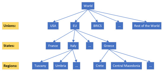
Figure 1.
The world tree structure at Union, State and Region Levels.
The division of regions and levels of localness shown in Figure 1 is based on political, economic and geographical criteria. In most cases, it reflects consumers’ perceptions of what is considered local in relation to them. However, there are still cases where consumers’ perceptions do not follow this specific pattern. For example, very large geographical areas may be inhabited by people who have no economic or other links with each other, so localness has to be defined at an even lower level. Regions of countries or islands very far from the mainland may be inhabited by people who consider neighbouring countries to be more local to them than the country to which they belong politically. Immigrants living and working in a country may feel more local to their place of origin than to their place of work. A different division can be defined to study such special cases. In any case, measuring localness with the ELI model goes beyond simply identifying companies on the basis of geographical proximity. It mainly involves assessing the economic contribution of companies to the regional economy, regardless of their geographical location.
According to the ELI model, the Level Localness Indicators () should be calculated for each financial entity. If the tree structure of Figure 1 contains, e.g., 5 unions, 50 states/countries, and 500 regions, each financial entity should have 5 Localness Indicators for the union level, 50 Localness Indicators for the state/country level, and 500 Localness Indicators for the regional level. The calculations needed for these Indicators can be easily executed since data are available in information systems used nowadays by most companies.
4.3.1. Definition of Union-Level Localness Indicator
The definition of the time-dependent Localness Indicator given by Equation (4) is extended in order to include the levels of localness concept and to first define the Union Level Localness Indicator as follows in Equation (5):
where N, j, t, T, y, , symbolise the same as in Equation (4), U declares the Union-Level Localness Indicator, u is the index (e.g., from 1 to 10) that defines a certain union of the tree structured model, and is the Union Level Localness Indicator for the entity j in year y in union u.
For example, let us assume that the world is divided into only three unions () and a company pays equal expenses per year to only three () entities as presented in Table 5, Table 6 and Table 7.
Table 5.
The expenses of a company to the first () of the entities for the previous years () and the first entity’s values of Union Localness Indicators for all unions and the previous 10 years.
Table 6.
The expenses of a company to the second () of the entities for the previous years () and the second entity’s values of Union Localness Indicators for all unions and the previous 10 years.
Table 7.
The expenses of a company to the third () of the entities for the previous years () and the third entity’s values of Union Localness Indicators for all unions and the previous 10 years.
In this example, the selected entities have the following characteristics. The first entity () is local for union 1 and its localness has increased over the years. The specific values are shown in Table 5. The second entity () localness is balanced to the three unions and the corresponding Union Localness Indicators are more or less similar. The specific values are shown in Table 6. The third entity () has Union Localness Indicators which are more or less similar for the first two unions and 0% for the third union. The specific values are shown in Table 7.
By using Equation (5) and the typical weights as in Table 2, the Union Localness Indicators for the company can be calculated for the three Unions and for six years from to the current year t, as presented in Table 8. For every year, historical data from the previous 5 years are needed.
Table 8.
The Union Localness Indicator calculated values of the company, for the three Unions and six years ().
The greater and increasing values of the Union Localness Indicator for Union 1, presented in Table 8, are justified by the greater and increasing values of the Union 1 localness of the first entity. The small values of the Union Localness Indicator for Union 3, presented in Table 8, are justified by the zero values of the Union 3 localness of the third entity.
Let us assume that in year the company is not satisfied with the value (71.7%) of the Union Localness Indicator for Union 1 () and wants to increase it. It decides to change the entity with another entity with higher values of the Localness Indicator in Union 1 (for example, it changes a supplier with a more local one for Union 1). The expenses paid to the new entity () are equal to the expenses that were paid in entity in the previous example. The expenses and the Union Localness Indicators () of entity 4 for the previous 5 years are presented in Table 9.
Table 9.
The expenses of a company to the entity () for 5 years () and its Union Localness Indicators for 5 years.
This change in the supplier has an impact on the calculated Union Localness Indicators of the company, as presented in Table 10. This example shows that a change in a company’s strategy, such as choosing to cooperate with local companies, increases the corresponding Localness Indicator of the company. In addition, this increase in the Localness Indicator is gradual because its calculation uses appropriately weighted historical data.
Table 10.
The Union Localness Indicator calculated values for the three Unions and six years () after changing entity with entity .
In Table 10, the percentage of each union shows how local the company is for each union. For the current year , the company is 86.3% local for Union 1, 44.1% local for Union 2 and 16.9% local for Union 3.
4.3.2. Definition of State-Level Localness Indicator
Similarly with the Union Level, the State-Level Localness Indicator can be defined as follows in Equation (6):
where N, j, t, T, y, , symbolise the same as in Equation (4), S declares the State-Level Localness Indicator, s is the index (e.g., from 1 to 50) that defines a certain state/country of the tree structured model, and is the State-Level Localness Indicator for the entity j in year y in state s.
4.3.3. Definition of Region-Level Localness Indicator
Similarly, the Region-Level Localness Indicator can be defined as follows in Equation (7):
where N, j, t, T, y, , symbolise the same as in Equation (4), R declares the Region-Level Localness Indicator, r is the index (e.g., from 1 to 500) that defines a certain region of the tree structured model, and is the Region-Level Localness Indicator for the entity j in year y in region r.
4.4. The Initialisation Process
Since all the definitions of the Union-, State- and Region-Level Localness Indicators are recursive, their calculation for a specific company needs the knowledge of the respective Level Localness Indicators of all the entities that are paid by the company. This is a condition that cannot always be realised for many reasons. At the start of the implementation of the ELI model for a company, or even during its implementation, the needed values of the Expenses Localness Indicators of some of the financial entities paid by the company may not be available. It is also possible that some of the financial entities that are paid are newly established and do not have historical data to apply the model, or they could be individuals or other types of companies that do not keep the required information.
In order to overcome this problem two different options could be followed. The first is to use the physical address of a company or individual to define the localness of it, as in Equation (2). This could be a good approximation of the truth for small companies. If the expenses data are not available, e.g., for individuals, fixed values could be used. For example, if the Region-Level Localness Indicator is set to 80% for the region where an individual lives, it means that this person pays 80% of its expenses in other financial entities in this region. This is most relevant to cases where a lot of information regarding Localness Indicators is missing for the implementation of the model.
If we consider that the ELI model has been adopted by most companies, the missing information would come from a few financial entities that have chosen not to apply the model. So, in this case, the second option is to set the Localness Indicators of these financial entities to zero (considering them as non-local). This would have, as a consequence, a negative effect on the Localness Indicators of the company. In order to overcome this, the company would possibly reduce the probability of choosing these entities for cooperation, and over time, it will force the implementation of the ELI model by more financial entities.
For new companies that want to implement the ELI model as soon as possible, the typical weights of Table 2 could change in order to use the current available data over time. For example, when the company has data for only the previous year, the weight for this year could be 100%. Similarly, if the company has data for two, three or four previous years the remaining percentages of non-operating years could be proportionally shared to the other weights. Such an example is presented in Table 11.
Table 11.
Typical values of weight factors for a five-year period and the corresponding values after proportional sharing of the percentage of non-operation years.
The weights of Table 11 can be used to calculate the Union Localness Indicators of the company with data presented in Table 5, Table 6 and Table 7, for the remaining years (). The calculation of the Union Localness Indicator for the year will apply the weights of the second line of the Table 11 (4 operating years) and data from 4 previous years (). The calculation of the Union Localness Indicator for the year will apply the weights of the third line of the Table 11 and data from 3 previous years (), and so on. The calculation of the Union Localness Indicator for the year will apply only the weight of 100% on the data of . By using this process, the corresponding Union Localness Indicators are shown in Table 12.
Table 12.
The Union Localness Indicator calculated values for the three Unions and four years ().
5. Experiments and Results
In order to illustrate the functionality and characteristics of the ELI model, a set of synthetic data was created to simulate a virtual economic world where financial entities transact with each other. In this economic world, there are N active financial entities, each one located in one of R regions. These regions belong to S states that belong to U unions. In this experiment, the selected values were as follows: N = 100,000, R = 500, S = 50, U = 5. The distribution of financial entities into regions is uniform, as is the distribution of regions into states and states into unions. Consequently, each union comprises approximately 10 states, each state approximately 10 regions and each region approximately 2000 financial entities.
For each time period, each financial entity incurs expenses to other entities. The amount of each expense sums up all payments of the current time period to the specific entity. These expenses values come from a lognormal distribution, which is typically employed in economic analyses and ensures that the values will be positive and that high values are less probable. The lognormal parameters are the mean value of the underlying normal distribution () and the standard deviation of the underlying normal distribution (). The selected values, and , which are used in the experiments, result in lognormal distributions that give an average value of about 200, and therefore, the sum of the 100 expenses for every financial entity is about 20,000. These numbers may be considered to express any monetary unit.
Then, each expense should be matched to one entity. Wanting to create a world based on the localness of expenses, four thresholds are defined, which indicate the percentage of payments made in the same region, state, union, and in the rest of the world, respectively. For example, if , and , it means that 40% of the expenses will be paid to entities located in the same region as the entity in question. The value means that an extra 30% of the expenses will be paid to entities located in the same state but not in the same region as the entity in question. The total amount of expenses paid in the same state will be 70%. The value means that an extra 20% of the expenses will be paid to entities located in the same union but not in the same state as the entity in question. The total amount of expenses paid in the same union will then be . The rest of the expenses are paid in entities in other unions. It should be noted that the threshold values may vary from one financial entity to another but the sum of the values for every entity should always equal . These values serve to express the entity’s behaviour regarding the selection of partners. For example, the greater the extent to which the value of r is higher, the more the expenses are paid in neighboring entities.
In the first experiment, the world is created by using N = 100,000, R = 500, S = 50, U = 5. The values of for each entity come randomly from uniform distributions, with the following lower and upper limits: . Based on the selected limits, the probability for a financial entity to spend more in its own region is greater than its tendency to spend in other regions of its own state, and so on. The lower limit of r was set to 10 to ensure that every entity will pay some expenses to its own region. After the draw, the values of are normalised to have a sum of . In this experiment, the statistics (mean, standard deviation, minimum and maximum) of the values for all entities are presented in Table 13.
Table 13.
The mean, standard deviation, minimum and maximum of the values of r, s, u and w for all financial entities.
Although the means of r, s, u and w are close to the centres of the corresponding distributions, there are entities that have values that are quite far from the typical, e.g., there is one that has unusually low r: , , , , and another one that has unusually high w: , , , .
Then, expenses are drawn for every financial entity, based on the lognormal distribution with and , and they are matched to other entities so as to meet the values of r, s, u and w for the entity in question. At the end of this matching, every entity j has a specific attitude regarding localness based on its values of , , and . The expenses and their matching remain the same for all years in this experiment. For every year the dataset contains 10 million amounts of expenses to 10 million entities.
Then, the localness values for all regions, states and unions of all entities to their own and other regions, states and unions will be calculated. For the first year , the localness for every level () and every financial entity is calculated by using only the physical address of the entities as a criterion, following the initialisation process described in Section 4.4. For each entity, the region localnesses, state localnesses and union localnesses are calculated and announced. Then, for five successive years , the localness values are calculated by using Equations (5)–(7), using the weights of Table 11. The mean, standard deviation, minimum and maximum of the values of , and for all financial entities are presented in Table 14. Notice that in Table 14, the statistics are derived from the values of the localnesses of all the financial entities to their own region, state and union only and not to all regions, states or unions. Thus, these values express how local in their own region, state or union level, are the financial entities as a whole. Since the same rules are applied for the creation of the thresholds (r, s, u, w), no different behaviour is observed between regions, states or unions.
Table 14.
The mean, standard deviation (stdev), minimum (min) and maximum (max) of the values of , and for all financial entities during the years ().
The mean values of the localnesses are close to the expected ones (40%, 70%, 90%) based on the selected thresholds. The small differences are justified due to the random process. The localness is recalculated annually, based on the localness of other entities and the payments incurred towards them. It is essentially a weighted (expenses-based) average of the localness of entities, and the recursive process reduces the standard deviation and restricts the outliers (min and max values). In this world, all entities follow the same strategy regarding localness up to .
At , the initialisation process has ended. At , the financial entity X, selected as the one with the smallest value of region localness (which has ), decides to change its strategy in order to become more local at the regional level. The only way to manage this objective is to change the entities where it pays money. First, it decides to stop cooperating with entities outside its union and to substitute them with entities from its own region. The amount of expenses remains the same and no other change happens. Table 15 shows how the region localness of X increases in the year from 16.3% to 22.4%. This difference corresponds to only 50% of the effect of the decision because of the weight used. The rest of the effect will be incorporated during the next years. At , this entity decides to be more regional, stops cooperation with entities outside its own state and substitutes them with entities from its own region. Lastly, at , it also decides to stop cooperation with entities outside its own region and to substitute them with entities from its own region. All these decisions have a positive effect on the regional localness for the following years, as presented in Table 15.
Table 15.
The values of region localness for the financial entity X after the change in cooperating entities, during the years ().
In the second experiment, the entities will be categorised in two groups. The first group (Group A) will follow a more local strategy and will have high r values (around ) coming from a uniform distribution: . The second group (Group B) will follow a less local strategy and will have low r values (around ) coming from a uniform distribution: . Each region contains approximately the same number of entities from both groups. The localness calculations are executed as in the previous experiment. Table 16 presents the statistics of region localness for the two groups of entities and for all entities together.
Table 16.
The mean, standard deviation (stdev), minimum (min) and maximum (max) of the values of for all financial entities and separately calculated for the two groups, during the years ().
The mean value of region localness for the entities of Group A is about 80%, as was expected. These entities interact only with each other, and therefore, they maintain the value of 80% as region localness. Similarly, the mean value of region localness for the entities of Group B is about 20%, as was expected. These entities also interact only with each other, and therefore, they maintain the value of about 20% as region localness. In both cases, the outliers (with values near the limits of distributions) are smoothed out as they interact with entities that have common values. This is captured in the reduction in the standard deviation values and in the minimum and maximum values, which gradually come closer to the mean value for both groups.
Now, after , the initialisation process has ended. The financial entity Y selected as the one with the smallest value of region localness (which has ) decides to change its strategy in order to become more local at the regional level. The only way to manage this objective is to change the entities to whom it pays money. It decides to stop cooperating with entities of its own region with low region localness (which belong in Group B) and starts to cooperate with entities from its own region with high region localness (which belong in Group A). So, the paid entities from the same region (of which there are 5) are substituted by 5 entities randomly chosen from entities in the same region but belonging in Group A. The amount of expenses remains the same and no other change happens. Table 17 shows how the region localness of Y increases in the year from 12.7% to 20.9%. This difference corresponds to only 50% of the effect of the decision because of the weight used. The rest of the effect will be incorporated during the next years. Moreover, at , this entity decides to be more regional and decides to substitute all the remaining cooperating entities, outside its own region, state or union, with entities from Group A of its own region. These decisions have a positive effect on its regional localness for the following years. Table 17 presents how the region localness of Y increases in the following years from to . The last value (89.7%) is higher than the mean value of Group A, since entity Y pays all of its expenses in its own region.
Table 17.
The values of region localness for the financial entity Y after the change in cooperating entities, during the years ().
6. Discussion
The main motivation that led to development of the innovative Localness Indicators definitions of the ELI model, was to give decision-makers (consumers or managers) reliable information on the localness of companies, in order to include this as a decision-making parameter in the choice of purchasing a product or service.
Figure 2 presents a flowchart where the required information flows between databases, processes and decisions. The diamond-shaped decision block in the centre of the graph shows the decision by any Financial Entity (company, individual, organisation, etc.) to incur expenses to buy products or services, pay employees, taxes or any other payment. Each Financial Entity reaches this decision through a process where information from both inside the entity (internal information) and its external environment (external information) is utilised and combined. Internal information includes elements such as available funds, other needs, existing priorities and, in general, the entity’s strategic planning for the future. External information includes the prices at which the products or services to be purchased are offered, their quality and other characteristics. Localness is among the factors that play a role in the final decision, even in the current process (blue shapes). But, although localness is requested and is useful information for decision making, it lacks reliability and accuracy as it is based only on the location of a company and is often supported by misleading marketing techniques.
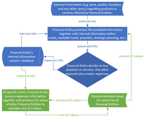
Figure 2.
The ELI model as a flowchart where the required information flows between databases, processes and decisions (current process in blue shapes, proposed extension in green shapes).
The adoption of the ELI model could have serious implications for the current decision-making process. The proposed definitions of Localness Indicators extend the flowchart by adding a process, an external database and the relative information flow, as shown in Figure 2 (green shapes). The new process will be applied at specific times (e.g., once a year or quarterly) in order to calculate the new ELI values of a Financial Entity by using its expenses information together with previous ELI values of the other Financial Entities. The expenses information is provided by the Financial Entity’s internal information system’s database. The previous ELI values are provided by the proposed external database that keeps the ELI values for all the Financial Entities. The new ELI values will also be kept in the same database. Moreover, this database provides current (new and previous) ELI values as reliable localness information which will be taken into account in the process that will lead to new buying and payment decisions.
For consumers to be able to use the ELI model in real life, the localness label needs to be defined as an end result that is usable by businesses and appealing to consumers. The type of label to be adopted as a localness indicator can be a percentage or an alphabetical scale and will be expressed by the label to be defined. The quick response code accompanying the token number on the product label can provide detailed information about the localness of the business. Stakeholders can easily obtain the localness information provided by the ELI model as identifiable information on the product label. Consumers will also be able to satisfy their need for local e-commerce products exclusively from transparent companies using the ELI model certification.
The primary outcome of this study is the definition of Expenses Localness Indicators at different levels of localness. The theoretical implications of this research follow. The ELI model supports localness strategies in enhancing the authenticity of companies in emerging markets [40,41]. This research highlighted the innovative use of information that already exists in the modern information systems used by most companies and organizations. This information can easily be used to add value to companies [73]. The ELI model also provides a transparent and verified means of assessing a company’s localness at different levels. This communication of proximity to consumers is useful in the policies of digital companies [46,47]. Communicating the results of the ELI model aims to create a connection with consumers, thus laying the foundation for sustainable longevity [22].
This research also has practical implications. A certified measurement of localness is useful both for companies that want to advertise their localness by asking for the support of the local community, and for consumers who want to modify their purchasing behaviour by taking into account reliable information on localness [36,37]. Similarly, in a B2B environment, a company that wants to maintain or increase its localness will take into account reliable information on the localness of other companies [48,49]. The ELI model enables financial entities to precisely measure their economic impact in a particular geographic area by analysing their historical expenses. The model has the potential to benefit society as a whole. It serves as a valuable tool for consumer teams to provide transparency to customers who are interested in knowing where their money goes when paying for products or services [27,31,83]. It provides objective evidence of community benefits, sustainability measurements, and social value. In the economic sector, it demonstrates the added value of contract work and local benefits and delivers auditable Corporate Social Responsibility [39]. Additionally, it provides professionals with the potential to promote local entrepreneurship [77]. Not-for-profit organisations could provide evidence of the value generated by grants and contracts for the local community. Furthermore, this model could assist international funders and foundations in evaluating the impact of grant aid and selecting projects that have the greatest local economic impact [44]. Furthermore, the local nature of the companies can be linked to environmental responsibility in the sense that the more local a company is, the less it engages in activities associated with unsustainable practices [55].
7. Conclusions, Limitations and Future Research
This paper defines and investigates the Expenses Localness Indicators (ELI) model, which introduces an innovative way to measure the localness of a company or any financial entity. The motivation for the development of the ELI model arose from the need to provide reliable information to consumers, managers and decision-makers more generally about localness, which leads to the creation of benefits for consumers, society and the economy.
The model was subjected to comprehensive testing on a large scale using appropriately structured synthetic data. The results demonstrated its efficacy in capturing diverse strategies with respect to localness.
Studies of consumer behaviour have shown that interest in localness is reinforced as a social attitude. The ELI model serves this social attitude by laying the foundation for rethinking the concept of local business, based on the idea that the more the company’s expenses are spent on local financial entities, the more the company increases its Localness Indicator. Thus, a business is local when the costs of its activities are spent on financial entities belonging to the specific area.
The ELI model offers society a reliable way to certify the localness of businesses that bypasses any third-party certification body. Governments, businesses and consumers with the proposed Localness Indicators have access to authentic information on the business’s localness. The Localness Indicators, by highlighting the local nature of businesses, enhance the creation of diversified products that contribute to the standard of living, income, employment, the use of local resources and, more generally, the prosperity of the region.
Consumers who want to trust local businesses must satisfy their need to know where their money is going. Reliable localness information could create a willingness to buy local products for supporting the local economy or satisfy consumer feelings of ethnocentrism and patriotism while, conversely, strengthening a reluctance to buy from opponent or offending nations or unions. Other factors influencing consumer behaviour can be taken into account by our model. This is a great advantage for the decision making of economic entities. For example, some groups of consumers may prefer to buy from a company that, while based in Greece, pays most of its expenses to entities located in Africa.
Moreover, the ELI model reveals new insights from the processing of information from companies’ and organisations’ information systems records. The use of modern information technologies promotes business excellence, as the optimisation of added value resulting from the optimal management of information leads to the measurement of Localness Indicators, related to the traceability of business expenses. Localness Indicators enable citizens, consumers, businesses, companies, organisations and governments to track the path of the money they spend on buying or investing or supporting or donating to companies or non-profit organisations, for collective benefit, to serve social interests, to alleviate suffering, to promote the interests of the poor, to protect the environment, or to provide basic social services.
The dynamic nature of the Expenses Localness Indicators is able to apply levels of localness, e.g., Regional, State/Country or Union levels and can influence the decision to spend in the defined localness level, enhancing the choice of local suppliers that contribute to the better value of the Indicator. Thus, companies can apply strategies that enhance the collaboration between local stakeholders. In addition, governments, local authorities and tourism operators can use the advantage of localness to positively enhance the image of an area as an attraction, serving tourism purposes. This enhances the promotion of the modern entrepreneurial and productive culture of each Region, State or Union.
However, this study is not without its limitations. The localness scores of the ELI model depend on data generated daily from the transactions of companies and individuals which, although not accessible to the research community—being in many cases subject to confidentiality laws—are collected by credit institutions and are usually submitted to government authorities for tax purposes. The required localness indicators can be easily calculated and published either by public authorities or by certified companies, without compromising the confidentiality of the transactions.
The full implementation of the proposed model on a large scale would require its acceptance by all states and the creation of a supranational framework so that each financial entity is accompanied by the localness indicators that characterise it, which is particularly difficult to achieve for political and/or economic reasons as the disclosure of this knowledge would not be in the interest of all companies and all states. However, by making the necessary assumptions, the model could be tested and, if supported by consumers and local or national governments interested in revealing local knowledge, it would encourage non-participating companies or states to gradually adopt the philosophy of the model.
The ELI model has been studied using synthetic data without taking into account the complex relationships between companies with many subsidiaries or branches, or with cooperating offshore companies, or for companies with extensive supply chains, and further research is recommended to generalise the findings to such special cases. Furthermore, while the results confirm that the model can measure localness in a consistent way, future studies could investigate how the model responds to economic shocks. Also, although the model appears to be quite robust, ways to trick the model with cosmetic data to improve the localness score need to be investigated more thoroughly.
Future work could also include extensive research to further study specific strategies for improving indicators at various levels. In addition, the application of the method using real data from large or small companies would be a trigger for the gradual adoption of the model by companies and consumers. The application of the model offers advantages and can be a strategic choice in many types of financial entities, such as local companies, hospitals, institutes or universities, other non-profit organisations or even international organizations.
The Localness Indicators which are defined through the ELI model satisfy all the research objectives that had been set. They can be applied to any financial entity, and include transactions coming either from domestic and cross-border e-commerce practices or from traditional transactions of purchasing goods or services. All Localness Indicators express localness as a percentage, taking values from 0% (non-local) to 100% (fully local). The main idea is fulfilled: The more a company pays money to local financial entities, the more its Localness Indicators will increase. The Localness Indicators are time-dependent and the use of proper weights is proposed to ensure smooth changes. Any company can draw up a policy, select their suppliers and/or employees and become more or less local over time. The definition of Localness Indicators has been extended to apply the concept at various levels, e.g., Regions, States or Unions. The proposed Localness Indicators provide reliable information to consumers and help them answer the questions: “where does my money go when I pay for a product or service?” or “how much of a product or service actually comes from the country it appears to be made in?”.
Author Contributions
Conceptualisation, methodology, validation and formal analysis, G.P. and V.C.; writing—original draft preparation, G.P.; writing—review and editing, V.C. All authors have read and agreed to the published version of the manuscript.
Funding
This research received no external funding.
Data Availability Statement
The data are available on request from the corresponding author.
Conflicts of Interest
The authors declare no conflicts of interest.
Abbreviations
The following abbreviations are used in this manuscript:
| B2B | Business to Business |
| ELI | Expenses Localness Indicators |
| EU | European Union |
| ICT | Information and Communication Technology |
| IoT | Internet of Things |
| PDO | Protected Designation of Origin |
| PGI | Protected Geographical Indication |
| USA | Unites States of America |
References
- Girgenti, V.; Massaglia, S.; Mosso, A.; Peano, C.; Brun, F. Exploring perceptions of raspberries and blueberries by Italian consumers. Sustainability 2016, 8, 1027. [Google Scholar] [CrossRef]
- Angowski, M.; Jarosz-Angowska, A. Local or Imported Product: Assessment of Purchasing Preferences of Consumers on Food Markets—The Case of Poland, Lithuania, Slovakia and Ukraine. Eurasian Stud. Bus. Econ. 2021, 11, 27–38. [Google Scholar] [CrossRef]
- Chousou, C.; Mattas, K. Assessing consumer attitudes and perceptions towards food authenticity. Br. Food J. 2019, 123, 1947–1961. [Google Scholar] [CrossRef]
- Cavite, H.J.; Mankeb, P.; Suwanmaneepong, S. Community enterprise consumers’ intention to purchase organic rice in Thailand: The moderating role of product traceability knowledge. Br. Food J. 2022, 124, 1124–1148. [Google Scholar] [CrossRef]
- Safeer, A.A.; Abrar, M.; Liu, H.; Yuanqiong, H. Effects of perceived brand localness and perceived brand globalness on consumer behavioral intentions in emerging markets. Manag. Decis. 2022, 60, 2482–2502. [Google Scholar] [CrossRef]
- Wang, E.; Gao, Z.; Heng, Y.; Shi, L. Chinese consumers’ preferences for food quality test/measurement indicators and cues of milk powder: A case of Zhengzhou, China. Food Policy 2019, 89, 101791. [Google Scholar] [CrossRef]
- Salnikova, E.; Grunert, K.G. The role of consumption orientation in consumer food preferences in emerging markets. J. Bus. Res. 2020, 112, 147–159. [Google Scholar] [CrossRef]
- Birtalan, I.L.; Neulinger, A.; Bárdos, G.; Rigó, A.; Rácz, J.; Boros, S. Local food communities: Exploring health-related adaptivity and self-management practices. Br. Food J. 2021, 123, 2728–2742. [Google Scholar] [CrossRef]
- Klade, M.; Seebacher, U.; Baumgartner, R.J. Life-Cycle-oriented Origin analysis—A method for calculating the geographical origin of products. J. Clean. Prod. 2015, 101, 86–96. [Google Scholar] [CrossRef]
- Imanova, G.E.; Imanova, G. Customer Characteristics in Digital Marketing Model. In International Conference on Theory and Applications of Fuzzy Systems and Soft Computing; Lecture Notes in Networks and Systems; Springer: Berlin/Heidelberg, Germany, 2023; Volume 610, pp. 164–171. [Google Scholar] [CrossRef]
- Tessitore, S.; Iraldo, F.; Apicella, A.; Tarabella, A. The Link between Food Traceability and Food Labels in the Perception of Young Consumers in Italy. Int. J. Food Syst. Dyn. 2020, 11, 425–440. [Google Scholar] [CrossRef]
- Shin Legendre, T.; Warnick, R.; Baker, M. The Support of Local Underdogs: System Justification Theory Perspectives. Cornell Hosp. Q. 2018, 59, 201–214. [Google Scholar] [CrossRef]
- Davvetas, V.; Halkias, G. Global and local brand stereotypes: Formation, content transfer, and impact. Int. Mark. Rev. 2019, 36, 675–701. [Google Scholar] [CrossRef]
- Cela, A.; Zhllima, E.; Skreli, E.; Imami, D.; Chan, C. Consumer preferences for goatkid meat in Albania. Stud. Agric. Econ. 2019, 121, 127–133. [Google Scholar] [CrossRef]
- Paun, C.; Ivascu, C.; Olteteanu, A.; Dantis, D. The Main Drivers of E-Commerce Adoption: A Global Panel Data Analysis. J. Theor. Appl. Electron. Commer. Res. 2024, 19, 2198–2217. [Google Scholar] [CrossRef]
- Tikhomirova, A.; Huang, J.; Chuanmin, S.; Khayyam, M.; Ali, H.; Khramchenko, D.S. How Culture and Trustworthiness Interact in Different E-Commerce Contexts: A Comparative Analysis of Consumers’ Intention to Purchase on Platforms of Different Origins. Front. Psychol. 2021, 12, 746467. [Google Scholar] [CrossRef]
- Hood, N.; Urquhart, R.; Newing, A.; Heppenstall, A. Sociodemographic and spatial disaggregation of e-commerce channel use in the grocery market in Great Britain. J. Retail. Consum. Serv. 2020, 55, 102076. [Google Scholar] [CrossRef]
- Nanda, A.; Xu, Y.; Zhang, F. How would the COVID-19 pandemic reshape retail real estate and high streets through acceleration of E-commerce and digitalization? J. Urban Manag. 2021, 10, 110–124. [Google Scholar] [CrossRef]
- Zhao, T.; Liang, Z.; Du, Y.; Huang, E.; Zou, Y. When Brands Push Us Away: How Brand Rejection Enhances In-Group Brand Preference. J. Theor. Appl. Electron. Commer. Res. 2024, 19, 3123–3136. [Google Scholar] [CrossRef]
- Wang, M.; Fan, X. An empirical study on how livestreaming can contribute to the sustainability of green agri-food entrepreneurial firms. Sustainability 2021, 13, 12627. [Google Scholar] [CrossRef]
- Marozzo, V.; Vargas-Sánchez, A.; Abbate, T.; D’Amico, A. Investigating the importance of product traceability in the relationship between product authenticity and consumer willingness to pay. Sinergie 2022, 40, 21–39. [Google Scholar] [CrossRef]
- Li, Q.; Tan, J.; Jiao, Y. Research on the formation mechanism of brand identification in cross-border e-commerce platforms—Based on the perspective of perceived brand globalness/localness. Heliyon 2024, 10, e25155. [Google Scholar] [CrossRef] [PubMed]
- Dionysis, S.; Chesney, T.; McAuley, D. Examining the influential factors of consumer purchase intentions for blockchain traceable coffee using the theory of planned behaviour. Br. Food J. 2022, 124, 4304–4322. [Google Scholar] [CrossRef]
- Morey, M. Preferences and the home bias in trade. J. Dev. Econ. 2016, 121, 24–37. [Google Scholar] [CrossRef]
- Kilders, V.; Caputo, V.; Liverpool-Tasie, L.S.O. Consumer ethnocentric behavior and food choices in developing countries: The case of Nigeria. Food Policy 2021, 99, 101973. [Google Scholar] [CrossRef]
- Bauer, B.C.; Johnson, C.D.; Singh, N. Place–brand stereotypes: Does stereotype-consistent messaging matter? J. Prod. Brand Manag. 2018, 27, 754–767. [Google Scholar] [CrossRef]
- Halimi, T.A. Examining the variation in willingness to buy from offending product’s origin among fellow nationals: A study from the Arab/Muslim-Israeli conflict. J. Islam. Mark. 2017, 8, 243–260. [Google Scholar] [CrossRef]
- Grashuis, J.; Magnier, A. Product differentiation by marketing and processing cooperatives: A choice experiment with cheese and cereal products. Agribusiness 2018, 34, 813–830. [Google Scholar] [CrossRef]
- Abraham, A.; Patro, S. ‘Country-of-Origin’ Effect and Consumer Decision-making. Manag. Labour Stud. 2014, 39, 309–318. [Google Scholar] [CrossRef]
- Brayden, W.C.; Noblet, C.L.; Evans, K.S.; Rickard, L. Consumer preferences for seafood attributes of wild-harvested and farm-raised products. Aquac. Econ. Manag. 2018, 22, 362–382. [Google Scholar] [CrossRef]
- Garza-Gil, M.D.; Vázquez-Rodríguez, M.X.; Varela-Lafuente, M.M. Marine aquaculture and environment quality as perceived by Spanish consumers. The case of shellfish demand. Mar. Policy 2016, 74, 1–5. [Google Scholar] [CrossRef]
- Safeer, A.A.; Zhou, Y.; Abrar, M.; Luo, F. Consumer Perceptions of Brand Localness and Globalness in Emerging Markets: A Cross-Cultural Context. Front. Psychol. 2022, 13, 919020. [Google Scholar] [CrossRef]
- Cheng, X.; Park, C. A Study on the Impact of Perceived Characteristics on Purchase Intention towards Collaboration Products between Foreign Brands and China Chic IPs. Glob. Bus. Financ. Rev. 2023, 28, 28–45. [Google Scholar] [CrossRef]
- Mandler, T.; Bartsch, F.; Han, C.M. Brand credibility and marketplace globalization: The role of perceived brand globalness and localness. J. Int. Bus. Stud. 2021, 52, 1559–1590. [Google Scholar] [CrossRef]
- Brüggemann, P.; Pauwels, K. How attitudes and purchases differ between also-online versus offline-only grocery shoppers in online and offline grocery shopping. Electron. Commer. Res. 2024. [Google Scholar] [CrossRef]
- Chen, J.; Liang, M.; Wei, Y. The influence of brand innovativeness on consumer purchase intentions towards domestic global brands in emerging markets: Evidence from China. J. Consum. Behav. 2023, 23, 1208–1218. [Google Scholar] [CrossRef]
- Davvetas, V.; Sichtmann, C.; Saridakis, C.; Diamantopoulos, A. The Global/Local Product Attribute: Decomposition, Trivialization, and Price Trade-Offs in Emerging and Developed Markets. J. Int. Mark. 2023, 31, 19–40. [Google Scholar] [CrossRef]
- Safeer, A.A.; Zhou, Y. Role of perceived brand globalness and localness in developing consumer word-of-mouth in the hospitality industry. Int. J. Emerg. Mark. 2025, 20, 259–277. [Google Scholar] [CrossRef]
- Götze, F.; Brunner, T.A. Sustainability and country-of-origin: How much do they matter to consumers in Switzerland? Br. Food J. 2020, 122, 291–308. [Google Scholar] [CrossRef]
- Safeer, A.A.; Chen, Y.; Abrar, M.; Kumar, N.; Razzaq, A. Impact of perceived brand localness and globalness on brand authenticity to predict brand attitude: A cross-cultural Asian perspective. Asia Pac. J. Mark. Logist. 2022, 34, 1524–1543. [Google Scholar] [CrossRef]
- Hoskins, J.; Verhaal, J.C.; Griffin, A. How within-country consumer product (or brand) localness and supporting marketing tactics influence sales performance. Eur. J. Mark. 2021, 55, 565–592. [Google Scholar] [CrossRef]
- Abrantes, B.F.; Ali, R.B. Perception of brand globalness and localness: The role of brand competence in stereotype-building and value consciousness. J. Mark. Anal. 2023, 11, 722–737. [Google Scholar] [CrossRef]
- Jung, J.M.; Jones, J.; Haugtvedt, C.P.; Banerjee, S. Consumer response to state-of-origin labels: The moderating role of residency. J. Consum. Mark. 2020, 37, 761–773. [Google Scholar] [CrossRef]
- Calderon-Monge, E.; Pastor-Sanz, I.; Sendra Garcia, F.J. Analysis of sustainable consumer behavior as a business opportunity. J. Bus. Res. 2020, 120, 74–81. [Google Scholar] [CrossRef]
- León Bravo, V.; Jaramillo Villacrés, M.; Silva, M.E. Analysing competing logics towards sustainable supplier management. Supply Chain. Manag. 2022, 27, 49–63. [Google Scholar] [CrossRef]
- Seidenfuss, K.U.; Kathawala, Y.; Dinnie, K. Assembly and component origin effects: An ASEAN consumer perspective. J. Consum. Mark. 2010, 27, 488–498. [Google Scholar] [CrossRef]
- Berg, N.; Preston, K.L. Willingness to pay for local food?: Consumer preferences and shopping behavior at Otago Farmers Market. Transp. Res. Part Policy Pract. 2017, 103, 343–361. [Google Scholar] [CrossRef]
- Anaza, N.A.; Kemp, E.; Osakwe, C.N.; Adeola, O. B2B brand marketing in Africa? An exploratory investigation of B2B buyers’ perception of supplier brands. Ind. Mark. Manag. 2023, 109, 90–105. [Google Scholar] [CrossRef]
- Mohan, M.; Brown, B.P.; Sichtmann, C.; Schoefer, K. Perceived globalness and localness in B2B brands: A co-branding perspective. Ind. Mark. Manag. 2018, 72, 59–70. [Google Scholar] [CrossRef]
- Lee, R.; Lockshin, L.; Greenacre, L. A memory-theory perspective of country-image formation. J. Int. Mark. 2016, 24, 62–79. [Google Scholar] [CrossRef]
- Lee, R.; Khan, H.; Bellman, S. Mere association of product image and travel destination. Ann. Tour. Res. 2021, 86, 103062. [Google Scholar] [CrossRef]
- Gagneten, A.M.; Regaldo, L.; Carriquiriborde, P.; Reno, U.; Kergaravat, S.V.; Butinof, M.; Agostini, H.; Alvarez, M.; Harte, A. Atrazine characterization: An update on uses, monitoring, effects, and environmental impact, for the development of regulatory policies in Argentina. Integr. Environ. Assess. Manag. 2023, 19, 684–697. [Google Scholar] [CrossRef] [PubMed]
- Penca, J.; Said, A.; Cavallé, M.; Pita, C.; Libralato, S. Sustainable small-scale fisheries markets in the Mediterranean: Weaknesses and opportunities. Marit. Stud. 2021, 20, 141–155. [Google Scholar] [CrossRef] [PubMed]
- Sadílek, T. Utilization of Food Quality Labels Included in the European Union Quality Schemes. Int. J. Food Syst. Dyn. 2020, 11, 72–83. [Google Scholar] [CrossRef]
- Van der Borght, K.; Gao, J.; Song, X. Geographical indications for agricultural products and foodstuffs in the EU: To what extent does the protection level match the scope of the subject matter? Queen Mary J. Intellect. Prop. 2021, 11, 270–294. [Google Scholar] [CrossRef]
- Luzak, J. A broken notion: Impact of modern technologies on product liability. Eur. J. Risk Regul. 2020, 11, 630–649. [Google Scholar] [CrossRef]
- Hasanzade, V.; Elshiewy, O.; Toporowski, W. Consumer Preferences and Their Willingness to Pay for Local Products (by Means of Consumer Ethnocentrism): An Abstract. In From Micro to Macro: Dealing with Uncertainties in the Global Marketplace; Springer: Berlin/Heidelberg, Germany, 2022; pp. 255–256. [Google Scholar] [CrossRef]
- Sampalean, N.I.; Rama, D.; Visentin, G. An investigation into italian consumers’ awareness, perception, knowledge of european union quality certifications, and consumption of agri-food products carrying those certifications. Bio-Based Appl. Econ. 2021, 10, 35–49. [Google Scholar] [CrossRef]
- Kim, E.H.; Lyon, T.P. Greenwash vs. Brownwash: Exaggeration and undue modesty in corporate sustainability disclosure. Organ. Sci. 2015, 26, 705–723. [Google Scholar] [CrossRef]
- Chen, Q.; Duan, Y. Impact of information disclosure on global supply chain greenwashing: Is more information transparency always better? Transp. Res. Part E Logist. Transp. Rev. 2023, 178, 103288. [Google Scholar] [CrossRef]
- Wei, Z.; Alam, T.; Al Sulaie, S.; Bouye, M.; Deebani, W.; Song, M. An efficient IoT-based perspective view of food traceability supply chain using optimized classifier algorithm. Inf. Process. Manag. 2023, 60, 103275. [Google Scholar] [CrossRef]
- Senthilkumar, G.; Tamilarasi, K.; Kaviarasan, S.; Arun, M. Trusty authentication of devices using blockchain-cloud of things (B-CoT) for fulfilling commercial services. Int. J. Syst. Assur. Eng. Manag. 2022. [Google Scholar] [CrossRef]
- Bader, L.; Pennekamp, J.; Matzutt, R.; Hedderich, D.; Kowalski, M.; Lücken, V.; Wehrle, K. Blockchain-based privacy preservation for supply chains supporting lightweight multi-hop information accountability. Inf. Process. Manag. 2021, 58, 102529. [Google Scholar] [CrossRef]
- Liu, Z.; Li, Z. A blockchain-based framework of cross-border e-commerce supply chain. Int. J. Inf. Manag. 2020, 52, 102059. [Google Scholar] [CrossRef]
- Lin, T.; Huan, Z.; Shi, Y.; Yang, X. Implementation of a Smart Contract on a Consortium Blockchain for IoT Applications. Sustainability 2022, 14, 3921. [Google Scholar] [CrossRef]
- Angara, J.S.; Saripalle, R.S. Towards a virtual water currency for industrial products using blockchain technology. Water Policy 2022, 24, 923–941. [Google Scholar] [CrossRef]
- Penco, L.; Serravalle, F.; Profumo, G.; Viassone, M. Mobile augmented reality as an internationalization tool in the “Made In Italy” food and beverage industry. J. Manag. Gov. 2021, 25, 1179–1209. [Google Scholar] [CrossRef]
- Jiang, J.; Chen, J. Managing the product-counterfeiting problem with a blockchain-supported e-commerce platform. Sustainability 2021, 13, 6016. [Google Scholar] [CrossRef]
- Hartley, J.L.; Sawaya, W.; Dobrzykowski, D. Exploring blockchain adoption intentions in the supply chain: Perspectives from innovation diffusion and institutional theory. Int. J. Phys. Distrib. Logist. Manag. 2022, 52, 190–211. [Google Scholar] [CrossRef]
- Montecchi, M.; Plangger, K.; Etter, M. It’s real, trust me! Establishing supply chain provenance using blockchain. Bus. Horizons 2019, 62, 283–293. [Google Scholar] [CrossRef]
- Aoudji, A.K.N.; Avocevou-Ayisso, C.; Adégbidi, A.; Gbénou, C.; Lebailly, P. Upgrading opportunities in agricultural value chains: Lessons from the analysis of the consumption of processed pineapple products in southern Benin. Afr. J. Sci. Technol. Innov. Dev. 2017, 9, 729–737. [Google Scholar] [CrossRef][Green Version]
- Zhou, J.; Jin, Y.; Liang, Q. Effects of regulatory policy mixes on traceability adoption in wholesale markets: Food safety inspection and information disclosure. Food Policy 2022, 107, 102218. [Google Scholar] [CrossRef]
- Cacchiarelli, L.; Carbone, A.; Laureti, T.; Sorrentino, A. The value of the certifications of origin: A comparison between the Italian olive oil and wine markets. Br. Food J. 2016, 118, 824–839. [Google Scholar] [CrossRef]
- Vanany, I.; Mardiyanto, R.; Ijtihadie, R.M.; Andri, K.B.; Engelseth, P. Developing electronic mango traceability in Indonesia. Supply Chain. Forum 2016, 17, 26–38. [Google Scholar] [CrossRef]
- Etwaroo, D.H.; Goburdhun, D.; Ruggoo, A. Classes of food additives in food products sold in Mauritius. Br. Food J. 2019, 121, 1125–1139. [Google Scholar] [CrossRef]
- Galli, F.; Brunori, G. Sustainability Performance of Food Chains: Linking Biodiversity and Nutritional Value in Italian Wheat-to-Bread Chains. Adv. Food Secur. Sustain. 2017, 2, 137–163. [Google Scholar] [CrossRef]
- Schmitt, E.; Galli, F.; Menozzi, D.; Maye, D.; Touzard, J.M.; Marescotti, A.; Six, J.; Brunori, G. Comparing the sustainability of local and global food products in Europe. J. Clean. Prod. 2017, 165, 346–359. [Google Scholar] [CrossRef]
- Sacks, J. The Money Trail: Measuring Your Impact on the Local Economy Using LM3; New Economics Foundation: London, UK, 2002. [Google Scholar]
- Kłoczko-Gajewska, A.; Malak-Rawlikowska, A.; Majewski, E.; Wilkinson, A.; Gorton, M.; Tocco, B.; Was, A.; Saïdi, M.; Török, A.; Veneziani, M. What are the economic impacts of short food supply chains? A local multiplier effect (LM3) evaluation. Eur. Urban Reg. Stud. 2023, 31, 281–301. [Google Scholar] [CrossRef]
- Tausl Prochazkova, P.; Noskova, M. An application of input-output analysis to social enterprises: A case of the Czech Republic. J. Entrep. Emerg. Econ. 2020, 12, 495–522. [Google Scholar] [CrossRef]
- Filippini, R.; Arfini, F.; Baldi, L.; Donati, M. Economic Impact of Short Food Supply Chains: A Case Study in Parma (Italy). Sustainability 2023, 15, 11557. [Google Scholar] [CrossRef]
- Donati, M.; Wilkinson, A.; Veneziani, M.; Antonioli, F.; Arfini, F.; Bodini, A.; Amilien, V.; Csillag, P.; Ferrer-Pérez, H.; Gkatsikos, A.; et al. Economic Spill-Over of Food Quality Schemes on Their Territory. J. Agric. Food Ind. Organ. 2021, 19, 95–111. [Google Scholar] [CrossRef]
- Graciotti, A.; McEachern, M.G. Rural space and the local food landscape: Consumers’ construction of food localness through the politics of belonging. J. Place Manag. Dev. 2024, 17, 1–20. [Google Scholar] [CrossRef]


Disclaimer/Publisher’s Note: The statements, opinions and data contained in all publications are solely those of the individual author(s) and contributor(s) and not of MDPI and/or the editor(s). MDPI and/or the editor(s) disclaim responsibility for any injury to people or property resulting from any ideas, methods, instructions or products referred to in the content. |
© 2025 by the authors. Licensee MDPI, Basel, Switzerland. This article is an open access article distributed under the terms and conditions of the Creative Commons Attribution (CC BY) license (https://creativecommons.org/licenses/by/4.0/).