Abstract
In the rapidly evolving domain of finance, quantitative stock selection strategies have gained prominence, driven by the pursuit of maximizing returns while mitigating risks through sophisticated data analysis and algorithmic models. Yet, prevailing models frequently neglect the fluid dynamics of asset relationships and market shifts, a gap that undermines their predictive and risk management efficacy. This oversight renders them vulnerable to market volatility, adversely affecting investment decision quality and return consistency. Addressing this critical gap, our study proposes the Graph Learning Spatial–Temporal Encoder Network (GL-STN), a pioneering model that seamlessly integrates graph theory and spatial–temporal encoding to navigate the intricacies and variabilities of financial markets. By harnessing the inherent structural knowledge of stock markets, the GL-STN model adeptly captures the nonlinear interactions and temporal shifts among assets. Our innovative approach amalgamates graph convolutional layers, attention mechanisms, and long short-term memory (LSTM) networks, offering a comprehensive analysis of spatial–temporal data features. This integration not only deciphers complex stock market interdependencies but also accentuates crucial market insights, enabling the model to forecast market trends with heightened precision. Rigorous evaluations across diverse market boards—Main Board, SME Board, STAR Market, and ChiNext—underscore the GL-STN model’s exceptional ability to withstand market turbulence and enhance profitability, affirming its substantial utility in quantitative stock selection.
1. Introduction
Quantitative stock selection uses knowledge from statistics, computer science, and finance to create models for selecting stock portfolios. The goal is to achieve returns that exceed benchmark rates. With the development of big data and cloud computing technologies, financial time series data exhibit more complex characteristics, including high dimensionality, strong volatility, and a large scale. Consequently, quantitative investment techniques are evolving from traditional strategies to modern artificial intelligence technologies, such as machine learning and deep learning.
Quantitative stock selection methods based on modern AI can be broadly categorized into machine learning and deep learning approaches. Machine learning methods, including random forest [1], gradient boosting [2], and support vector machines (SVMs) [3], are trained on features and historical statistical characteristics without considering data temporality. These models face performance limitations with large-scale, unstructured, or high-dimensional data. They struggle to capture the complex, nonlinear patterns in stock markets. Deep learning methods, represented by recurrent neural networks (RNN) [4] and long short-term memory (LSTM) networks, can process sequential data directly [5]. Compared to traditional linear models, these deep learning approaches offer significant improvements. They are more effective in predicting stock price movements, identifying market opportunities, and constructing automated trading systems. Transformers, known for handling long-term dependencies in sequential data, have emerged as another focal point for time series forecasting. Some researchers have explored hybrid models that combine neural networks with statistical methods to enhance financial forecasting accuracy [6]. Despite the progress made in deep learning-based quantitative stock selection, challenges still remain due to the high dimensionality, volatility [7], and complex interrelations of financial time series. Most existing models handle stocks or assets in isolation, overlooking potential correlations and interactions. This results in the lack of a relational modeling perspective. Recent studies leveraging graph neural networks have sought to address this issue, but reliance on subjective graph construction may distort input information. Also, the lack of focus on the importance of individual stocks reduces the accuracy of graph node representations. Moreover, integrating relational modeling with the sequential nature of time series data remains an area for improvement.
To tackle these challenges, we propose the Graph Learning Spatial–Temporal Encoder Network (GL-STN) model. This model effectively addresses the high dimensionality, strong volatility, and complex correlations of financial time series data by using graph embedding learning, modeling temporal and spatial relationships.
The GL-STN model overcomes the limitations of existing models by introducing innovative methods for graph learning and spatial–temporal encoding. It effectively addresses the high dimensionality and volatility of financial data and captures the complex interrelations between stocks.
Unlike traditional machine learning models that struggle with large-scale, unstructured, or high-dimensional data, GL-STN excels by modeling the intricate dependencies and temporal dynamics of financial markets. While conventional neural network models focus on sequential data processing, GL-STN integrates graph convolutional neural networks with LSTM to capture both spatial relationships and temporal dependencies. This dual capability allows for a more comprehensive analysis of market data. Moreover, compared to existing graph neural network models, GL-STN reduces subjective factors in the graph construction process. It accurately determines the importance of each stock node through attention mechanisms, enhancing the accuracy of node representations. This multi-faceted approach ensures unprecedented accuracy and robustness in financial market analysis.
Furthermore, the GL-STN model’s multi-layered and multi-module architecture enables processing and analyzing data from multiple perspectives and dimensions. This facilitates comprehensive multi-modal feature extraction and processing while maintaining flexibility and scalability. Consequently, the GL-STN model can easily extend and adapt to incorporate additional data sources or new analytical techniques. This flexibility results in unprecedented accuracy and stability.
Key contributions include constructing a network graph that learns and establishes relationships between stocks, effectively capturing their interactions and dependencies. This approach addresses the oversight of stock correlations in traditional models. Additionally, graph convolutional neural networks and attention mechanisms [8] process graph structural information, extracting features and the importance of individual stocks for more accurate feature aggregation. Furthermore, by integrating LSTM, the model enhances its ability to capture temporal dependencies, facilitating the learning of features across time and space. Comparative analyses with mainstream machine learning and neural network models across various financial markets validate the effectiveness of the proposed model.
2. Related Work
2.1. Quantitative Investment Techniques Based on Machine Learning
Machine learning methods excel in model transparency and interpretability. They can demonstrate high efficiency and reliability when dealing with small-scale or structured data. However, these methods often rely on feature engineering. They struggle to identify and utilize complex patterns and relationships hidden within the data. Wang S. [9] showcased the significant effectiveness of the random forest model in the stock market. Li B. et al. [10] used various machine learning models, including multiple neural networks, to construct different investment portfolios. Empirical tests showed annual returns significantly outperforming the market index. Zhou L. [11] confirmed the superiority of multi-factor stock selection models over traditional linear regression models through the study of six major categories of factors. Shu S. [12] created SCAD-logistic regression and MCP-logistic regression models by altering the penalty function in the logistic regression model, showing notable application effects in the stock market. Lewellen [13] successfully predicted excess returns of stocks by integrating 15 factors using the FM regression method. DeMiguel et al. [14] approached this topic from the perspective of investor utility, finding six company characteristics that could independently predict average returns. The utility-based models were practically applied in stock market prediction. Gu et al. [15] tested common machine learning algorithms in the U.S. market, finding that machine learning models could effectively outperform traditional linear regression models. Yu et al. [16] developed a support vector machine model to predict stock market trends. By using genetic algorithms to select attributes, the complexity of support vector machines can be reduced while improving modeling efficiency. In terms of classification performance, it can surpass traditional time series and neural network models. Based on intelligent media and technical analysis, Mndawe et al. [17] developed a stock price prediction framework, focusing on the application of machine learning in stock market prediction.
2.2. Quantitative Investment Techniques Based on Deep Neural Networks
By learning nonlinear changes in high-dimensional features, deep neural networks offer better representational capabilities than traditional methods. They can provide powerful analytical tools for quantitative investment. Despite challenges in model interpretability, the performance in prediction accuracy and efficiency has garnered widespread attention. Recent studies have shown significant progress in applying deep learning technology to quantitative stock selection strategies. Lin J. and Gong Z. [18] built convolutional neural network and BP neural network models based on the prices of Shanghai zinc futures, emphasizing the effectiveness of neural networks in stock price prediction. Liu et al. [19] proposed a quantitative option trading strategy based on convolutional neural networks. It is possible to exceed benchmark indices and basic momentum strategies by combining CNN predictions of stock prices with LSTM’s quantitative timing strategy. Liang et al. [20] used long short-term memory networks to extract time series features and predict the trend of rebar futures prices. They found that using LSTM for feature extraction and the XGBoost model to filter trading signals generated by trading strategies can effectively improve annualized returns. Kim et al. [21] proposed a paired trading method combining deep reinforcement learning, enhancing the efficiency and profitability of trading strategies. Staffini [22] utilized the application of deep convolutional generative adversarial networks in stock price prediction, exploring the application of generative adversarial networks in financial market analysis.
The introduction of an attention mechanism provides new breakthroughs in the application of deep learning in quantitative investment strategies. Liu H et al. [23] explored how to use attention mechanisms to enhance the efficiency and effectiveness of quantitative investment strategies. By combining sequential graph structures with attention mechanisms, Lai et al. [24] developed new deep learning modules aimed at capturing and analyzing time series data more accurately.
2.3. Quantitative Investment Techniques Based on Graph Models
By constructing complex networks among financial assets, graph models [25] reveal the structure and dynamic changes in the market. They can provide a unique perspective for quantitative investment. In graph models, each asset in the financial market is treated as a node, and interactions between assets are represented by edges within the network. This model is particularly suitable for analyzing complex systems in financial markets, revealing potential associations and mutual influences between assets. Wang Z. et al. [26] aimed to address complex relationships and data challenges in financial markets by classifying financial graphs and outlining graph neural network (GNN) methods. In order to propose a continuous learning factor predictor based on graph neural networks, Tan Z. et al. [27] focused on the challenges of future price prediction in high-frequency trading. By combining multi-factor pricing theory with real-time market dynamics, the limitations of existing methods in ignoring trend signals and interactions can be effectively overcome.
3. GL-STN
3.1. Model Framework
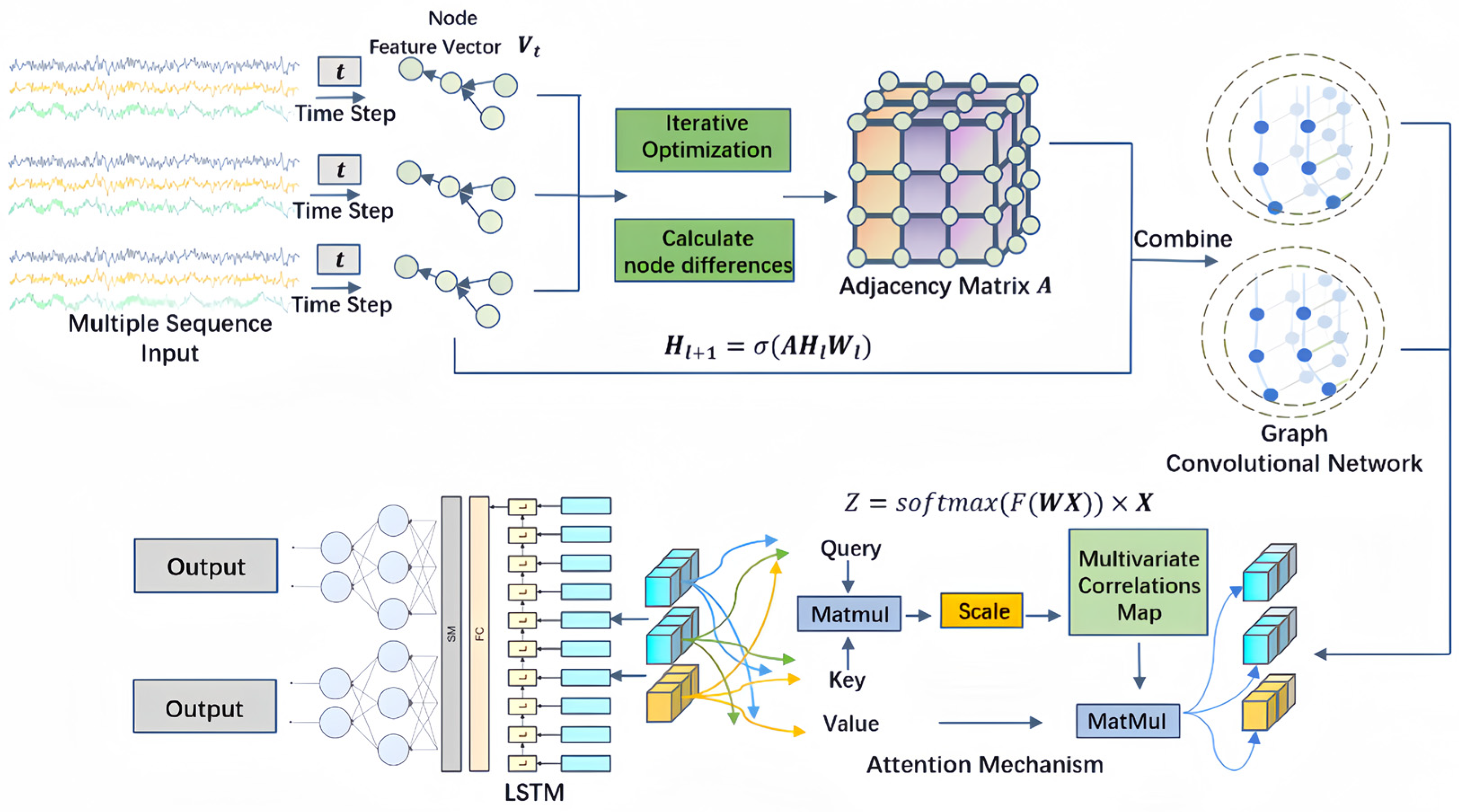
The framework of the GL-STN model, as shown in Figure 1, is divided into three modules: graph embedding, a graph convolutional network (GCN), and RNN, presenting a sequential relationship. The input sequence data represent the dynamic features of stocks. The nodes corresponding to each sequence are assigned a feature vector to represent the state of each strand. Initially, the feature vectors are iteratively optimized to compute the differences between nodes to construct an adjacency matrix. This step allows the model to utilize the graph’s representational capability to map the correlations between individual stocks. Subsequently, the adjacency matrix and feature vectors are input into the GCN. Within the GCN, an attention mechanism is integrated to learn the importance distribution of different nodes across stocks, enhancing the model’s precision in quantitative stock selection. Finally, the output from the GCN is passed to the LSTM to capture the temporal evolution patterns of stock features. By combining multiple layers and mechanisms, GL-STN generates outputs that provide observable support for subsequent quantitative stock selection.
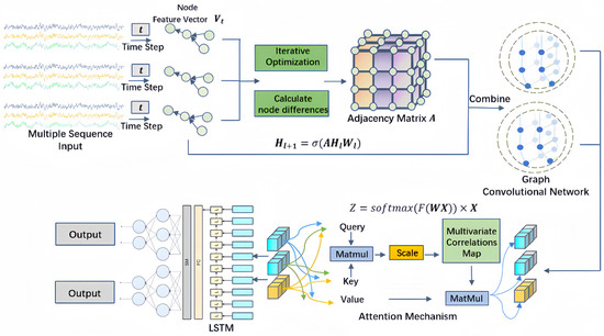
Figure 1.
GL-STN schematic diagram.
3.2. Model Algorithm
The algorithm of the GL-STN model is shown in Algorithm 1. Firstly, we initialize the primal variable w and the dual variable v, and set the initial number of nodes N. Subsequently, the algorithm generates a vectorized representation of matrix H by calculating the Euclidean distance between each row of the feature matrix. This step captures the spatial relationships of the data, which is crucial for analyzing the spatiotemporal characteristics of stock market data. Following this, the primal variable w and the dual variable v are iteratively updated to ensure the model can effectively adapt to the dynamic changes in the market. Finally, the output from the GCN is processed through an attention mechanism. This allows the model to focus on key features to enhance the accuracy and efficiency of predictions.
| Algorithm 1. GL-STN (PDS unrolling) |
| Input: Feature matrix , number of unrolling times , input dimension # Initialize primal variable w, dual variable v, and set the initial number of nodes N based on the shape of V |
|
3.3. Multi-Sequence Input
The model framework introduces a multi-sequence input to process the multidimensional characteristics of the stock market. Each sequence represents specific attributes of stock data, such as the price, trading volume, market indicators, etc. Sequences are preprocessed and transformed into node feature vectors at time step t. The multi-dimensional sequence input strategy enables the GL-STN model to comprehensively capture various aspects of the stock market. It can provide a detailed data foundation for the graph structure analysis phase.
3.4. Graph Learning
To reveal the latent connections among stock data, we refer to the Learning to Graph (L2G) theory [28]. Node feature vectors is used to learn the graph adjacency matrix [29,30]. reveals the latent connections between stock market assets. Subsequently, the adjacency matrix is normalized to produce , as shown in Equation (1), where is the degree matrix derived by summing each row of .
After constructing the normalized network, the network features and asset feature matrix are combined. Asset trends are estimated through a linear combination layer with parameters θ. θ and b are weights learned during training. The output trend estimation is shown in Equation (2).
Finally, the sign function is applied to to produce trading signals , as shown in Equation (3). This step transforms trend estimates into trading decisions, building a network-based trading strategy.
The application of graph learning enhances the accuracy of stock data analysis, addressing the inadequacies in considering the interconnectivity among individual stocks [31].
3.5. Graph Convolution
In the GL-STN model, GCN is used to analyze complex interactions in stock market data [32,33]. The model’s core objective is to extract key features from graph data to deeply understand the influences between nodes. Initially, the adjacency matrix is calculated based on historical data between stocks. Then, the model performs graph convolution operations by combining the node feature vectors at each time step t with the adjacency matrix , as shown in Equation (4). represents the node feature matrix of the lth layer, while denotes the corresponding weight matrix. The activation function σ is used to help the model learn complex feature representations.
The graph convolution operation can be simplified, as shown in Equation (5), because we use linear activation functions in the model. The feature representation of a node is determined solely by the weighted sum of its neighbors’ features, without introducing additional nonlinear transformations.
Through GCN operations, the GL-STN model generates updated feature representations for each node, reflecting the stock’s relative position and potential market influence in the network [34]. It is crucial for understanding the network role value of each stock.
3.6. Attention Mechanism
The GL-STN model incorporates an attention mechanism to enhance the model’s ability to capture and express important information [35,36]. Firstly, linear layers are applied to process the output of GCN. Then, attention coefficients are calculated to generate attention weights for each node, as shown in Equation (6). represents the node features output by the graph convolutional network, is the weight matrix of the linear layer, is a linear transformation function. By using the function, the output of the linear layer is normalized into a probability distribution.
Subsequently, the GL-STN model aggregates the node features weighted by the calculated attention coefficients, as seen in Equation (7). The × symbol represents element-wise multiplication, and is the weighted node feature representation.
Through the attention mechanism, the GL-STN model can accurately identify and emphasize key node features, thereby precisely capturing individual stock characteristics and enhancing the accuracy of the feature aggregation phase.
3.7. Temporal Processing
In the GL-STN model, the GCN output weighted by the attention mechanism is fed into the LSTM [37] layer. This enables the model to combine the complex relationships between nodes revealed by the GCN. It also accounts for the dynamic changes in the temporal dimension. LSTM processes inputs over time steps with its recursive structure, retaining memory of past information, thereby extracting richer and deeper features. Subsequently, the output from the LSTM layer is passed to a fully connected layer to form the final prediction result.
The core of the LSTM lies in its cell state and three gate mechanisms (forget gate, input gate, and output gate), which together manage the storage and removal of information. The forget gate determines the information to be retained, the input gate updates the cell state, and the output gate controls the output of the hidden state. Specifically, the gate structure of the LSTM is defined as shown in Equations (8)–(12), where , , , , and represent the input gate, forget gate, memory cell, output gate, and hidden state:
By incorporating LSTM, the GL-STN model significantly improves in recognizing and analyzing the temporal dependencies of data, achieving comprehensive feature learning of stock data in both the temporal and spatial dimensions. This provides strong support for quantitative stock selection.
4. Experimental Evaluation
4.1. Experimental Data
The data we used were sourced from the Tushare platform, covering stocks listed on the Main Board, SME Board, STAR Market, and ChiNext Market from 1 June 2023 to 10 December 2023. Specifically, our dataset encompassed daily trading records of a diverse array of stocks from these different markets, ensuring a comprehensive and representative sample. The Main Board and SME Board collectively include 3201 stocks, generating an aggregate daily trading data volume of 323,721 records. The STAR Market comprises 566 stocks, adding an additional 52,423 daily trading records. The ChiNext Market includes 1332 stocks, contributing a further 152,769 daily trading records. The extensive collection captures the full breadth of market dynamics, providing a robust and solid foundation for our model. For effective training and evaluation, the dataset was divided into a training set (1 June 2023, to 1 August 2023), a validation set (2 August 2023, to 10 August 2023), and a test set (11 August 2023, to 10 December 2023). The model inputs included trading information and derived technical indicators, as detailed in Table 1. By analyzing the input features, the model outputted probability values indicating the likelihood of stock price increases. This approach offered precise estimations of stock market dynamics.

Table 1.
Stock data input by the model.
4.2. Experimental Setup
4.2.1. Experimental Platform
The GL-STN model we propose is implemented using Python 3.5 and the PaddlePaddle framework. All reference models are also implemented using the same tools. The hardware environment for the experiments includes a system with a Tesla V100 GPU, a quad-core CPU, 32 GB of video memory, 32 GB of RAM, and 100 GB of disk storage space. The model training period is set to 1000 epochs, with a fixed learning rate of 0.00001, and each batch contains 190 samples. The loss function for all models involving neural networks is BCEWithLogitsLoss [38], and the optimizer used is AdamW [39].
4.2.2. Baseline Model Comparison
Considering the structural characteristics of the current Chinese stock market, comparative experiments were conducted on the Main Board and SME Board, STAR Market, and ChiNext Market.
The Main Market is a merger of the original Main Board and the SME Board, mainly traded on the Shenzhen Stock Exchange and the Shanghai Stock Exchange. It covers both large mature enterprises and small and medium-sized growth enterprises, representing the core and diversity of the Chinese stock market. The ChiNext Market, located at the Shenzhen Stock Exchange, focuses on supporting enterprises with strong growth potential and innovation capabilities. The STAR Market, located at the Shanghai Stock Exchange, is dedicated to supporting enterprises with core technologies and high innovation capabilities. These three segments collectively promote the diversified development of the Chinese stock market, playing a crucial role in market stability and innovation.
To comprehensively evaluate the effectiveness of the GL-STN model, we selected three representative gradient boosting models (LightGBM [40], CatBoost [41], XGBoost [42]) and three neural network models (LSTM [43], CNN-LSTM [44,45,46,47,48], Transformer [49,50]) for result comparison. Additionally, we conducted ablation experiments to compare the performance differences between three models: a simplified model with only the L2G layer (L2GMOM), an intermediate model combining the L2G layer and LSTM (L2GMOM_LSTM), and the full GL-STN model.
4.2.3. Evaluation Metrics
Evaluation metrics included periodic return, excess return, winning rate, maximum drawdown, Sharpe ratio, Sortino ratio, information ratio, alpha, and beta, defined as per Equations (13)–(21).
represents the initial capital, denotes the return, is the strategy’s annualized return rate, is the benchmark’s annualized return rate, and refers to the risk-free rate. Additionally, indicates the standard deviation of the portfolio’s annualized return rate, is the net value of the product on day i, and is the net value of the product on some day after . represents the downside standard deviation, α is the portfolio’s excess return, ω is the active risk, is the strategy’s daily return, and represents the benchmark’s daily return. is the number of winning trades and is the total number of trades.
4.3. Experimental Results and Analysis
4.3.1. Main Board and SME Board Experimental Results Comparison
The Main Board and SME Board markets are known for their mature trading environment and high volatility. Among the gradient boosting models, LightGBM leads in periodic return, with a performance of −0.0930, while CatBoost and XGBoost have return values of −0.1018 and −0.1484, respectively. However, the average winning rate of these models is only 0.3921, highlighting their limitations in providing effective trading decision support. Risk-adjusted return metrics, including average Sharpe ratio, Sortino ratio, and information ratio, are −2.1989, −3.5394, and −0.7376. These results further highlight the limitations in risk-adjusted returns and information generation, as shown in Table 2.

Table 2.
The performance of different models on various metrics based on Main Board and SME Board.
In neural network models, LSTM, CNN-LSTM, and Transformer show instability in maintaining account value with periodic return metrics of −0.0759, −0.1379, and −0.1309. The winning rate metrics highlight shortcomings in trading decision-making—0.3913 for LSTM, 0.3194 for CNN-LSTM, and 0.3846 for Transformer. The average information ratio for these three models is about −0.9868, suggesting deficiencies in providing efficient trading decisions and decision-supporting information, as shown in Table 2.
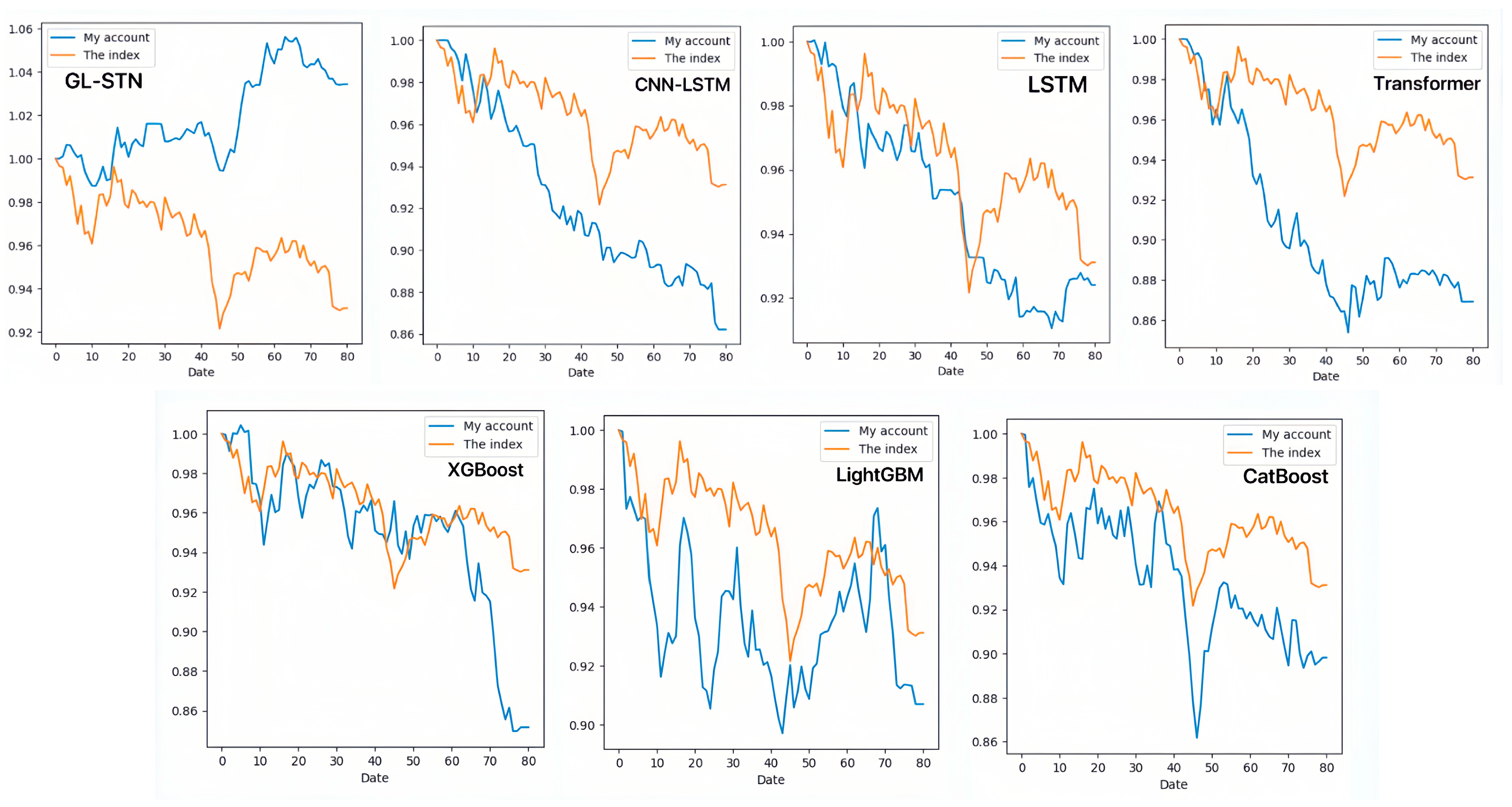
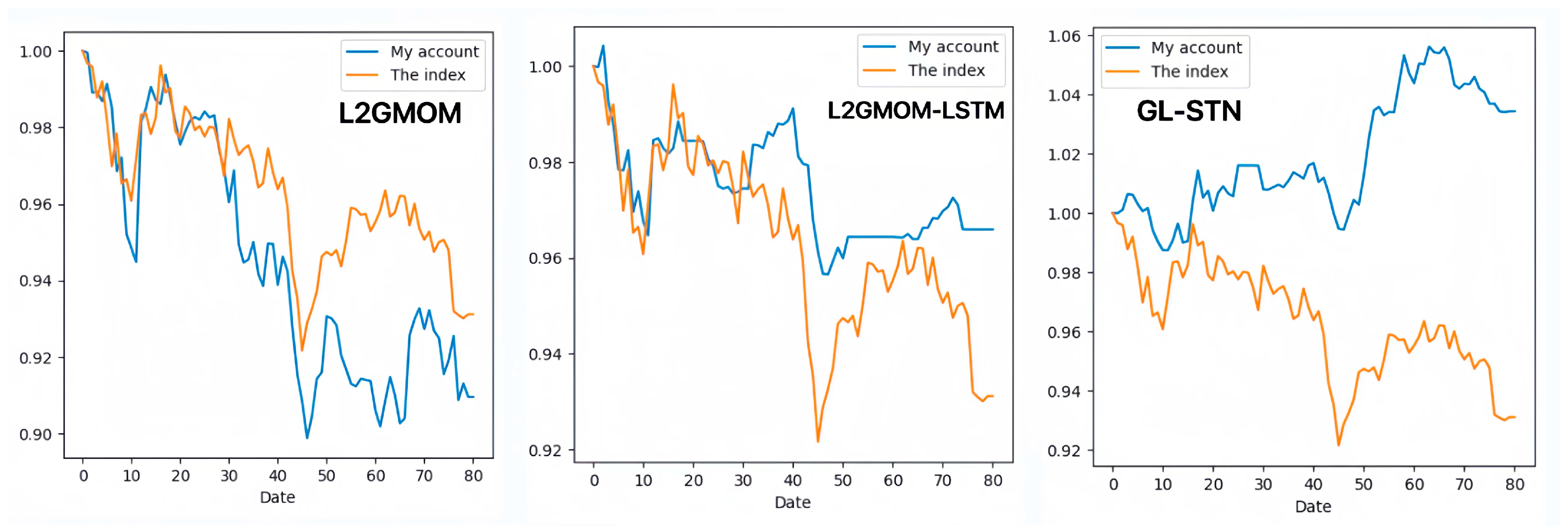
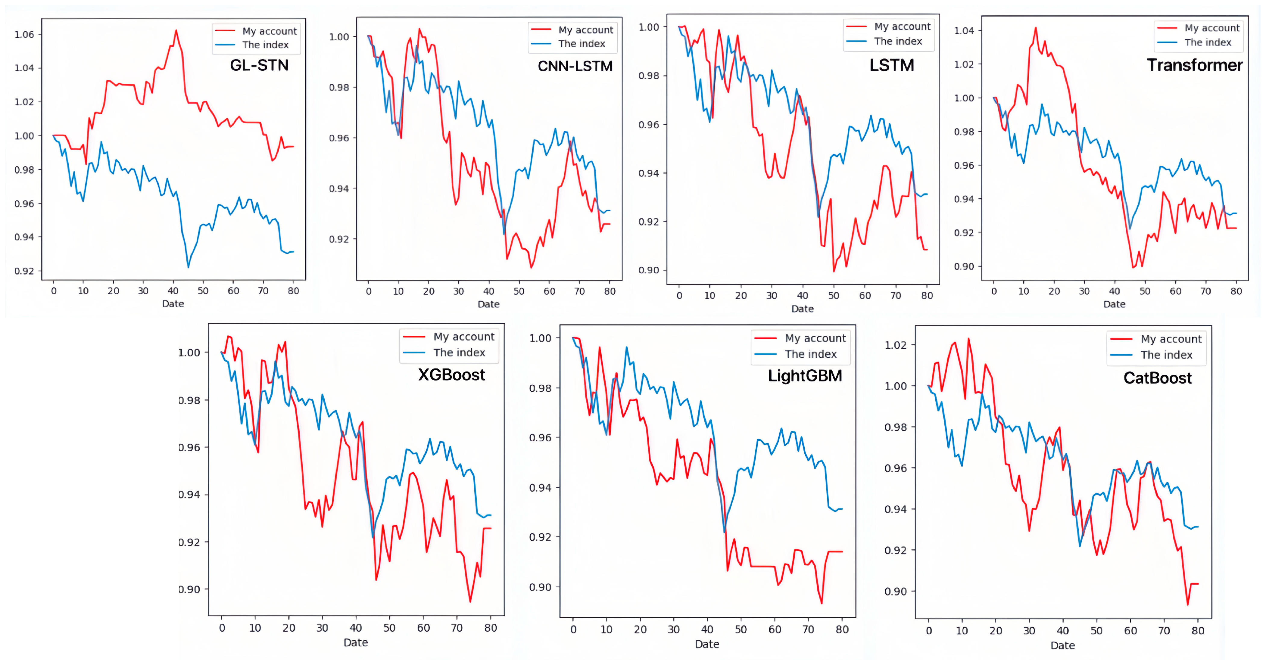
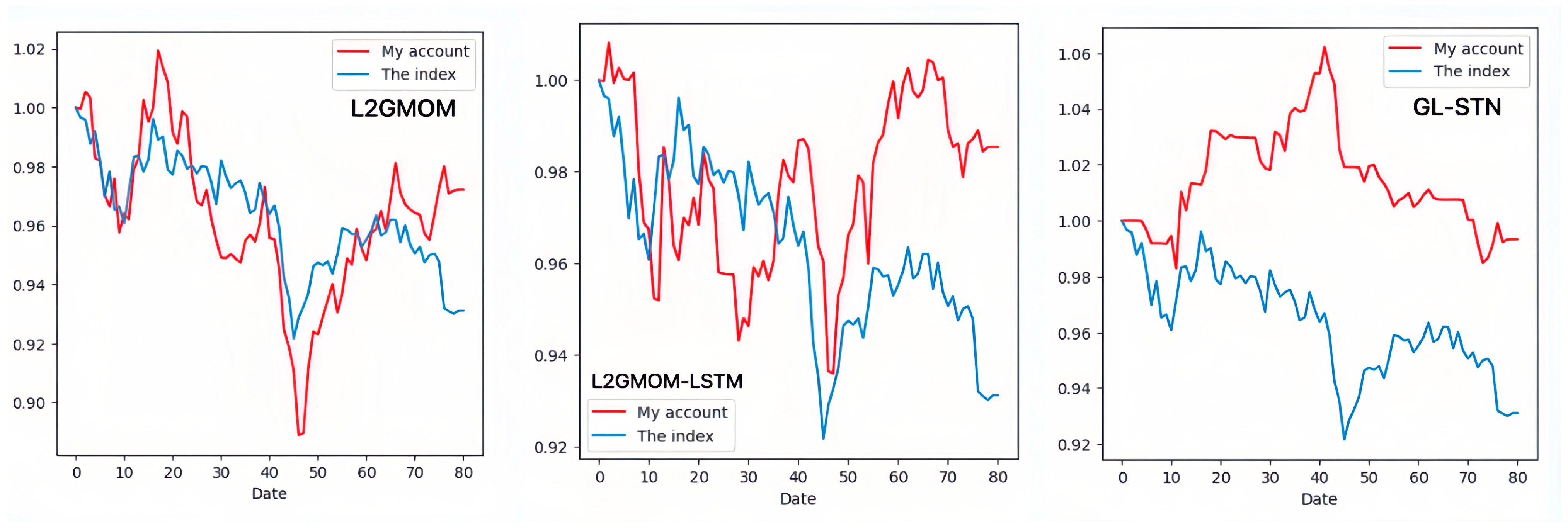
In contrast, the GL-STN model outperforms other models with a positive periodic return metric of 0.0343, demonstrating its performance in maintaining account value stability. Additionally, GL-STN achieves a winning rate of 0.5581, a maximum drawdown of only 0.0221, and significantly high values for the Sharpe ratio and Sortino ratio. The account value change curves of different models, as depicted in Figure 2, visually underscore the GL-STN model’s superior ability to sustain account value in the volatile markets of the Main Board and SME Board. Additionally, the ablation experiments, illustrated in Figure 3, demonstrate the efficiency and robustness of the GL-STN model in navigating market complexities. This is shown through the comparative account value change curves of the models under stringent tests. These experiments, as detailed in Table 3 and Table 4, affirm the GL-STN model’s standout performance and high efficiency.
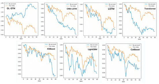
Figure 2.
The account value change curves of different models based on Main Board and SME Board.
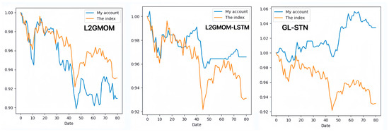
Figure 3.
The account value change curves of models in the ablation experiment based on Main Board and SME Board.

Table 3.
The performance of models in the ablation experiment on various metrics based on Main Board and SME Board.

Table 4.
Runtime of models in the ablation experiment based on Main Board and SME Board.
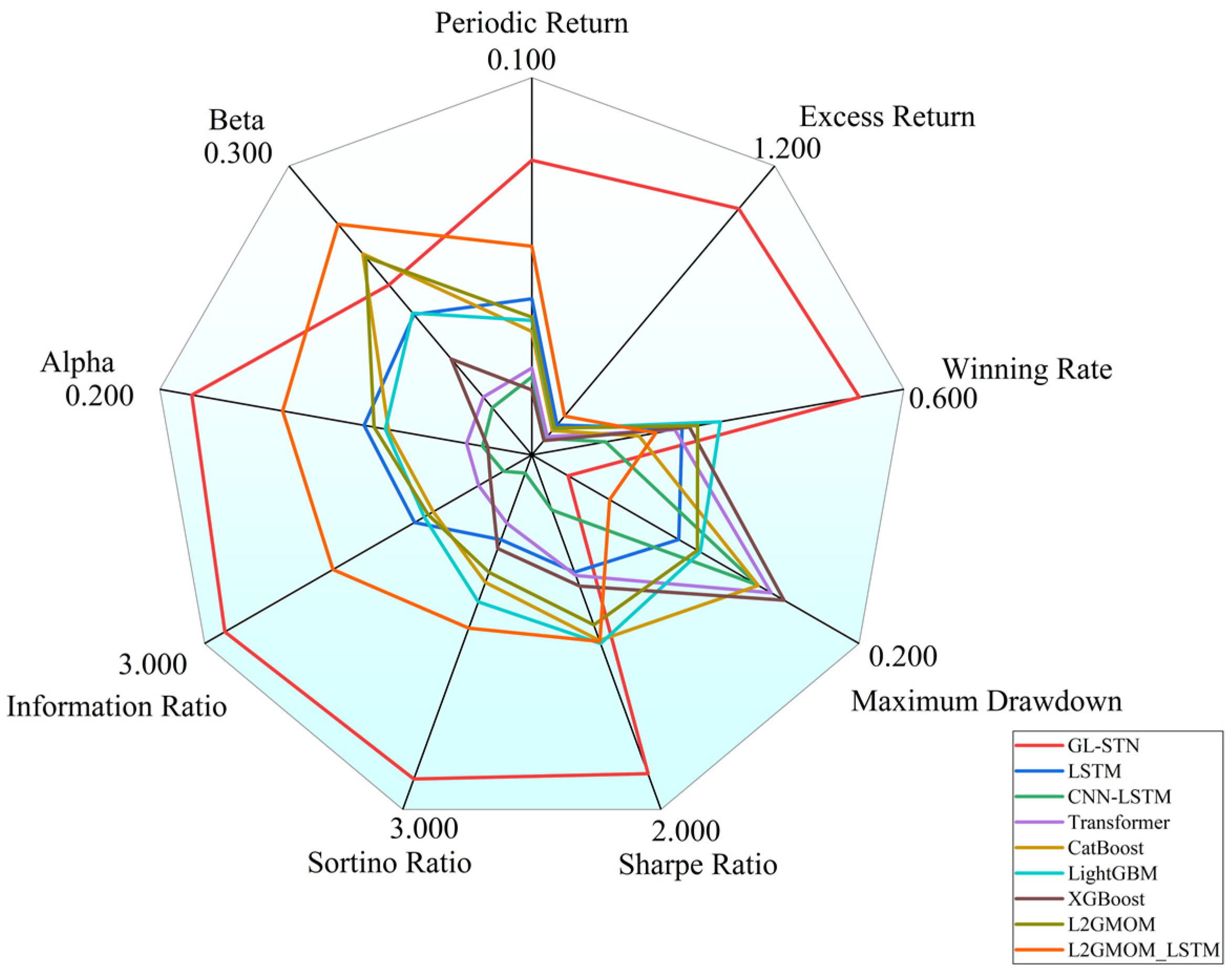
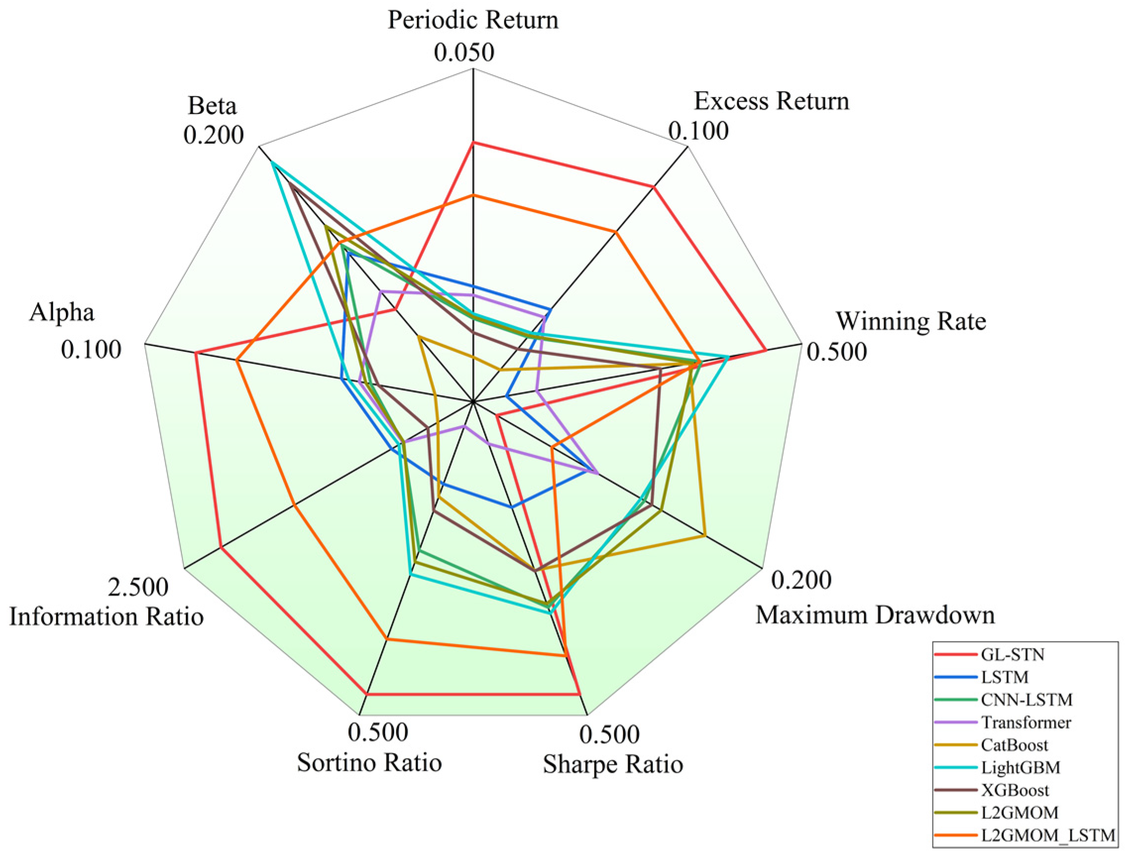
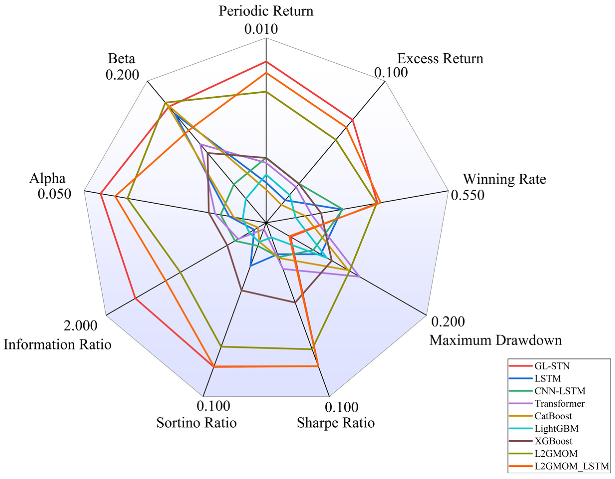
Moreover, Figure 4 provides a radar comparison chart, which succinctly contrasts the comprehensive metrics of various models, highlighting GL-STN’s outstanding performance across multiple dimensions, thereby reinforcing its superiority in navigating the complexities of high-volatility trading environments.
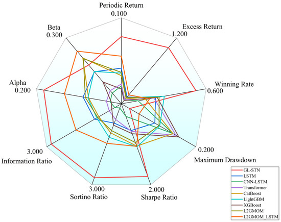
Figure 4.
Radar comparison chart of model metrics on Main Board and SME Board.
4.3.2. STAR Market Experimental Results Comparison
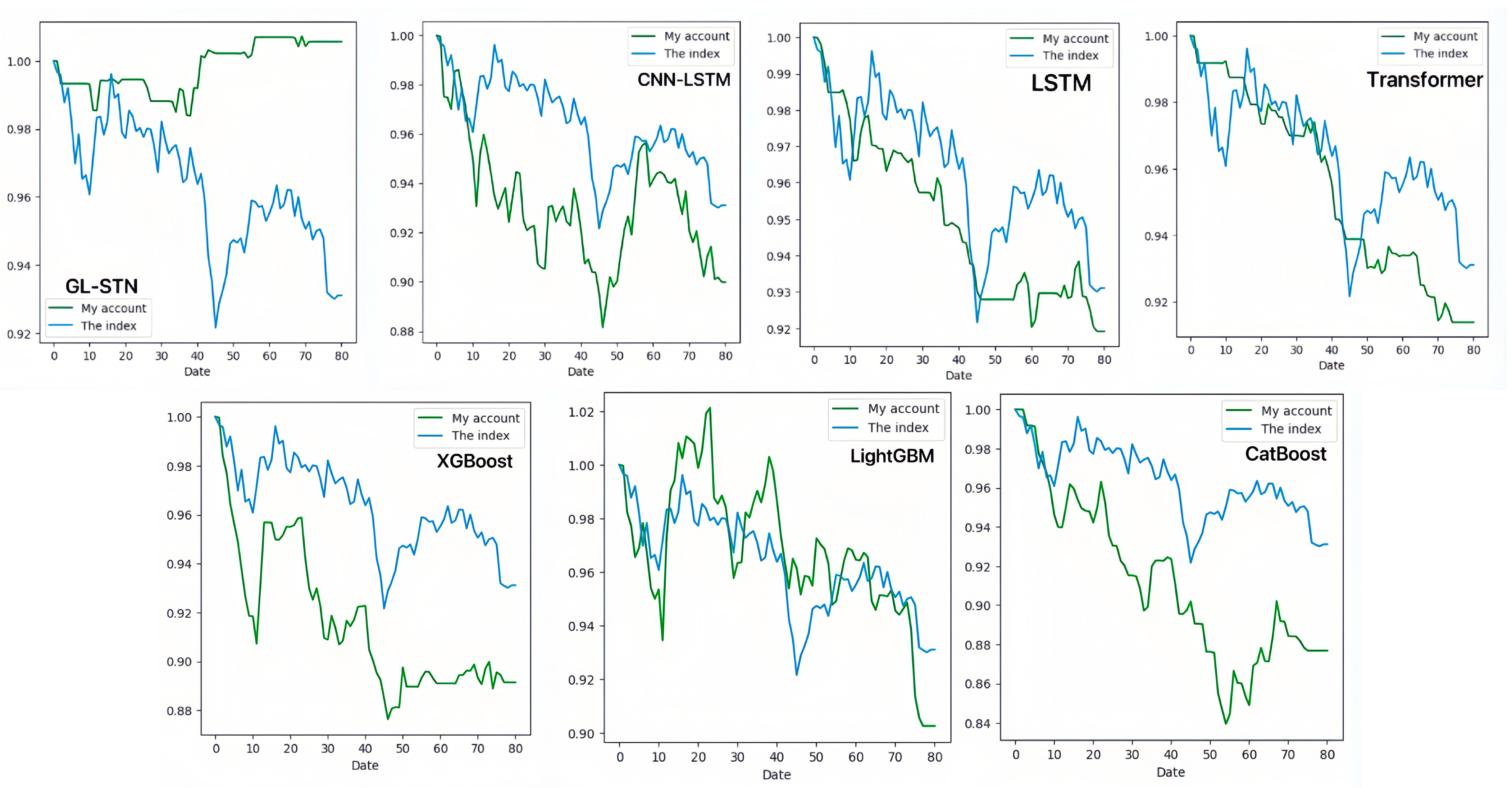
In the science and technology innovation-driven STAR Market, gradient boosting models (LightGBM, CatBoost, XGBoost) show limitations in decision-making quality amidst high volatility. All models exhibit negative periodic returns and an average trade win rate of approximately 0.3837. The Sharpe ratio, Sortino ratio, and information ratio averages of −2.6174, −4.0004, and −0.7846, respectively, underscore the challenges in achieving risk-adjusted returns and generating informative insights, as shown in Table 5.

Table 5.
The performance of different models on various metrics based on STAR Market.
Neural network models encounter similar hurdles in the STAR Market. The LSTM and CNN-LSTM models report periodic returns of −0.0808 and −0.1001, respectively, while the Transformer model slightly outperforms them at −0.0861. This performance indicates instability in maintaining account value, compounded by a low average trade winning rate of 0.2651 and an average information ratio of −0.4733. These results, shown in Table 5, highlight deficiencies in delivering precise trading strategies and supporting information.
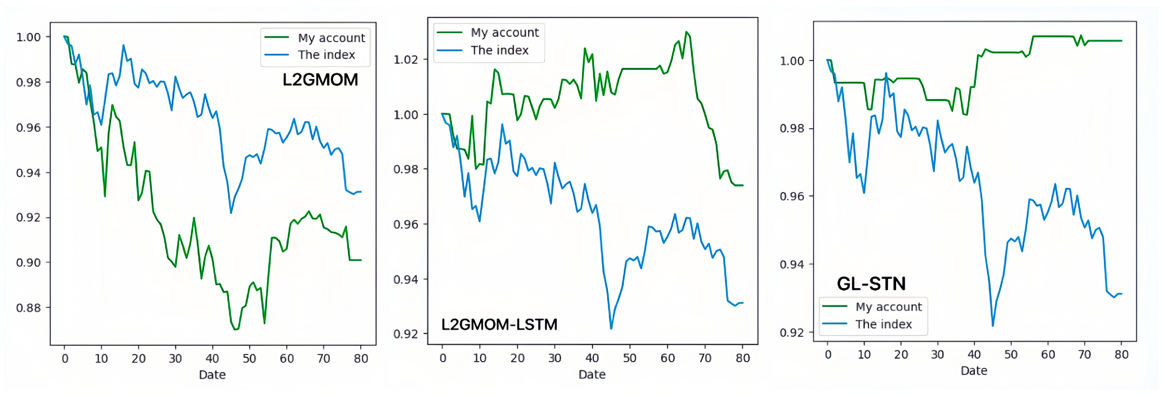
Contrastingly, the GL-STN model demonstrates exceptional stability in the STAR Market, reflected by a positive periodic return of 0.0056, a winning rate of 0.4615, and a maximum drawdown rate of 0.0162, alongside impressive Sharpe and Sortino ratios. Its performance distinctly surpasses that of other models, underlining its efficiency in decision-making, account value stability, and risk management. The account value change curves for different models on the STAR Market, illustrated in Figure 5 and Figure 6, visually emphasize the GL-STN model’s resilience and superior ability to maintain account value against its counterparts. Furthermore, Table 6 and Table 7 underscore the robustness of the GL-STN model in ablation studies conducted on the STAR Market. They also demonstrate its operational efficiency, with a runtime of only 4.7232 h. Figure 7’s radar comparison chart of model metrics on the STAR Market offers a comprehensive visualization of the GL-STN model’s outstanding performance across various dimensions, affirming its advanced capability in managing the intricacies of high-volatility trading environments.
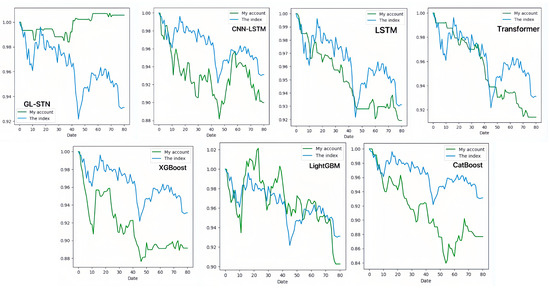
Figure 5.
The account value change curves of different models based on STAR Market.

Figure 6.
The account value change curves of models in the ablation experiment based on STAR Market.

Table 6.
The performance of models in the ablation experiment on various metrics based on STAR Market.

Table 7.
Runtime differences in models in the ablation experiment based on STAR Market.
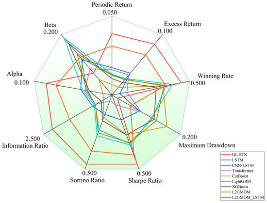
Figure 7.
Radar comparison chart of model metrics on STAR Market.
4.3.3. ChiNext Market Experimental Results Comparison
In the ChiNext Market, gradient boosting models have shown consistent performance in periodic return but overall poor effectiveness. LightGBM slightly outperforms the others with a result of −0.0861, while CatBoost and XGBoost achieve values of −0.0966 and −0.0744. Moreover, the average values for the Sharpe ratio, Sortino ratio, and Information ratio are −1.8532, −2.7696, and −0.2534, indicating deficiencies in profitability and information output after adjusting for risk, as shown in Table 8.

Table 8.
The performance of different models on various metrics based on ChiNext Market.
In the evaluation of neural network models, LSTM and CNN-LSTM failed to demonstrate stability in periodic return, while the Transformer model showed slight improvement with a fluctuation value of −0.0778. Additionally, the average trade winning rate for these models is only 0.4225, suggesting limited capability in providing efficient trading decision support. The average information ratio of −0.2145 further reveals the models’ inadequacy in delivering effective decision-support information, as shown in Table 8.
Conversely, the GL-STN model emerges as a standout in the ChiNext Market, showcasing significant stability and superior performance. It leads with a winning rate of 0.4722, underscoring its precision in trading decisions. It also exemplifies unparalleled loss control capabilities with a maximum drawdown rate of 0.0728. Furthermore, GL-STN’s superior Sharpe and Sortino ratios reflect its efficacy in securing higher returns at minimized risks. With an information ratio of 1.5242, GL-STN stands at the forefront, demonstrating its exceptional ability to outperform market benchmarks. The model’s excellence extends to the alpha and beta indicators, affirming its superior risk-adjusted returns and market adaptability.
The account value change curves for different models in the ChiNext Market, shown in Figure 8 and Figure 9, clearly highlight the GL-STN model’s robustness and consistent account value preservation, setting it apart from its peers. The ablation experiment results, as presented in Table 9 and Table 10, demonstrate that GL-STN outperforms both L2GMOM and L2GMOM_LSTM models in terms of its shorter running time and superior index benefits. This further substantiates its computational efficiency and exceptional performance. The comprehensive radar comparison chart in Figure 10 encapsulates the model metrics on the ChiNext Market, offering a succinct overview of GL-STN’s leading performance across various dimensions.
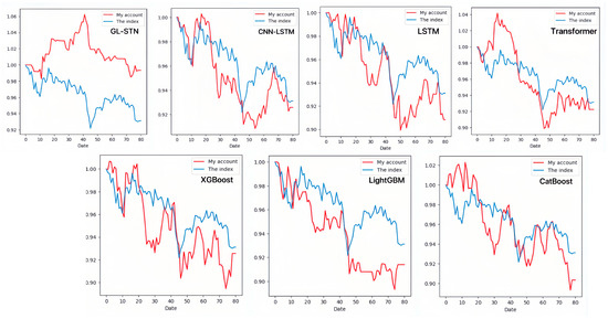
Figure 8.
The account value change curves of different models based on ChiNext Market.

Figure 9.
The account value change curves of models in the ablation experiment based on ChiNext Market.

Table 9.
The performance of models in the ablation experiment on various metrics based on ChiNext Market.

Table 10.
Runtime differences in models in the ablation experiment based on ChiNext Market.
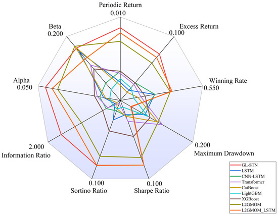
Figure 10.
Radar comparison chart of model metrics on ChiNext Market.
5. Discussion and Analysis
Building on the evaluation of the GL-STN model’s performance across different Chinese stock market segments, it is crucial to emphasize the Chinese stock market’s representativeness in the global financial landscape. As one of the world’s largest stock markets, the Chinese stock market is representative not only in terms of scale and liquidity but also in volatility, regulatory environment, market structure, and technological applications. It offers a comprehensive landscape for evaluating the GL-STN model and provides valuable insights into global financial markets.
Firstly, China’s Main Board market encompasses a large number of mature, large-cap companies. It has relatively low volatility and high liquidity, similar to the New York Stock Exchange (NYSE) and National Association of Securities Dealers Automated Quotations (NASDAQ) in the United States. The SME board mainly represents the investment environment for small and medium-sized enterprises, akin to the Frankfurt Stock Exchange (FSE) and other European stock markets. These markets offer an ideal environment for testing the model’s adaptability to different economic scales and types of enterprises. On the Main and SME Boards, the GL-STN model demonstrates effective market volatility control and strong profitability through lower cyclical returns and higher Sharpe ratios. These characteristics indicate that the GL-STN model has the potential to perform well in other mature markets with similar attributes globally.
Secondly, the STAR Market and ChiNext Market are characterized by high volatility and high growth, making them suitable for studying model performance in emerging market environments. Emerging markets such as India and Brazil also share these characteristics, with high innovation potential but also high risk. On the STAR Market, the GL-STN model maintains stable trading success rates and controlled maximum drawdowns. In the ChiNext Market, the GL-STN model shows good adaptability, effectively handling market volatility and risk management. This implies its potential applicability in other high-risk, high-reward markets worldwide. By testing in China’s diverse markets, we can better understand and predict the applicability and performance of the GL-STN model in other global markets.
Furthermore, abrupt market shifts and black swan events are crucial factors that cannot be ignored in quantitative stock selection. The GL-STN model incorporates certain measures in the hope of addressing these challenging issues. Firstly, through multi-sequence inputs, the GL-STN model can dynamically adapt to market changes, enhancing its sensitivity to sudden events. Secondly, GL-STN uses GCN to process complex interactions in stock market data, generating feature representations that reflect the relative positions and influences of stocks within the market network. This captures nonlinear and dynamic relationships, improving the model’s responsiveness to sudden changes. Additionally, the integrated attention mechanism significantly enhances the GL-STN model’s ability to capture and emphasize critical market information, allowing the model to focus on key market signals and maintain robustness in volatile markets. Finally, by combining LSTM to process weighted GCN outputs, GL-STN has the potential to quickly adjust predictions and decisions, demonstrating high flexibility and adaptability during sudden events or black swan incidents.
Moreover, the GL-STN model’s robust and complex design, which includes GCN, L2G mechanisms, attention mechanisms, and LSTM, is well-suited for handling large volumes of market data. This architecture effectively captures and analyzes both spatial and temporal features in financial datasets. The design of the GL-STN model facilitates high-dimensional data processing and robust feature extraction, ensuring precise analysis even with extensive and complex datasets.
Additionally, the model structure is highly extendable. Its architecture is designed to accommodate increasing data complexity and volume, making it capable of managing larger datasets and more intricate financial instruments. The modular approach, incorporating components such as GCN and LSTM, allows for the seamless integration of additional layers or mechanisms to enhance performance. This flexibility allows the GL-STN model to adapt to evolving market conditions, integrate new data sources, and incorporate advanced analytical techniques as they become available. Its extensibility supports continuous improvement and adaptation, ensuring its relevance and effectiveness in the ever-changing financial markets.
Overall, the evaluations suggest that the GL-STN model exhibits a degree of versatility and robustness. It shows potential in quantitative stock selection across diverse global markets, demonstrates the ability to handle large datasets, and may assist in managing abrupt market shifts and black swan events.
6. Conclusions and Outlook
The aim of this study was to explore a novel quantitative stock selection method based on the GL-STN model. We conducted an in-depth analysis of traditional quantitative stock selection methods and the principles of the L2G layer. By integrating GCN, L2G, attention mechanisms, and LSTM, we proposed an improved composite investment strategy. Empirical results demonstrate that in various market segments such as the Main Board, SME Board, STAR Market, and ChiNext Market, the GL-STN model exhibits significant stability, profitability, and excellent market adaptability.
In the mature Main and SME Boards, the GL-STN model effectively controlled market volatility and ensured profitability, with a lower periodic return and higher Sharpe ratio. In the volatile STAR Market, the model maintained a stable winning rate and controlled maximum drawdown. In the ChiNext market, it demonstrated strong adaptability in managing market fluctuations and risk.
Despite positive results, there remains room for improvement in model parameter optimization, feature selection, and time efficiency [51]. Future research could explore more efficient parameter adjustment methods and more refined feature engineering techniques to enhance the model’s accuracy and generalizability. Furthermore, although the GL-STN model has reduced runtime, there is still scope for further improvement in time efficiency. Additionally, while the current model focuses mainly on the Chinese stock market, future studies should apply it to international stock markets to explore the model’s performance in different market environments. This would not only validate the model’s robustness but also provide references for international quantitative investment strategies.
Author Contributions
T.C., conceptualization, methodology, software, writing—original draft; X.W., validation, software; H.W., data curation, resources; X.Y., project administration, supervision; L.X., conceptualization, methodology, writing—review and editing. All authors have read and agreed to the published version of the manuscript.
Funding
This work is supported by Philosophy and Social Science Planning Cross-disciplinary Key Support Subjects of Zhejiang Province (No. 22JCXK08Z), Ningbo Natural Science Foundation (No. 2022J162), Zhejiang Province Statistical Research Project (No. 23TJZZ22), Ningbo Philosophy and Social Science Research Base Project (No. JD6-228).
Institutional Review Board Statement
Not applicable.
Informed Consent Statement
Not applicable.
Data Availability Statement
The data presented in this study are available upon request from the first author.
Conflicts of Interest
The authors declare no conflicts of interest.
References
- Breiman, L. Random Forests. Mach. Learn. 2001, 45, 5–32. [Google Scholar] [CrossRef]
- Friedman, J.H. Greedy Function Approximation: A Gradient Boosting Machine. Ann. Stat. 2001, 29, 1189–1232. [Google Scholar] [CrossRef]
- Cortes, C.; Vapnik, V. Support-Vector Networks. Mach. Learn. 1995, 20, 273–297. [Google Scholar] [CrossRef]
- Rumelhart, D.E.; Hinton, G.E.; Williams, R.J. Learning Representations by Back-Propagating Errors. Nature 1986, 323, 533–536. [Google Scholar] [CrossRef]
- Zhao, H.; Wu, L.; Li, Z.; Zhang, X.; Liu, Q.; Chen, E. Prediction of Internet Financial Market Dynamics Based on Deep Neural Network Structure. J. Comput. Res. Dev. 2019, 56, 1621–1631. [Google Scholar]
- Shi, X.; Chen, Z.; Wang, H.; Yeung, D.Y.; Wong, W.K.; Woo, W.C. Convolutional LSTM Network: A Machine Learning Approach for Precipitation Nowcasting. Adv. Neural Inf. Process. Syst. 2015, 28, 802–810. [Google Scholar]
- Bollerslev, T. Generalized Autoregressive Conditional Heteroskedasticity. J. Econom. 1986, 31, 307–327. [Google Scholar] [CrossRef]
- Vaswani, A.; Shazeer, N.; Parmar, N.; Uszkoreit, J.; Jones, L.; Gomez, A.N.; Kaiser, Ł.; Polosukhin, I. Attention Is All You Need. Adv. Neural Inf. Process. Syst. 2017, 30, 5998–6008. [Google Scholar]
- Wang, S.; Cao, Z.; Chen, M. Research on the Application of Random Forest in Quantitative Stock Selection. Oper. Res. Manag. Sci. 2016, 25, 163–168+177. [Google Scholar]
- Li, B.; Lin, Y.; Tang, W. ML-TEA: A Set of Quantitative Investment Algorithms Based on Machine Learning and Technical Analysis. Syst. Eng.—Theory Pract. 2017, 37, 1089–1100. [Google Scholar]
- Zhou, L. Research on Multi-factor Stock Selection Strategy Based on Quantile Regression. J. Southwest Univ. Nat. Sci. Ed. 2019, 41, 89–96. [Google Scholar]
- Shu, S.; Li, L. Regularized Sparse Multi-factor Quantitative Stock Selection Strategy. Comput. Eng. Appl. 2021, 57, 110–117. [Google Scholar]
- Lewellen, J. The Cross-Section of Expected Stock Returns. Crit. Financ. Rev. 2015, 4, 1–44. [Google Scholar] [CrossRef]
- DeMiguel, V.; Martin-Utrera, A.; Nogales, F.J. A Transaction-Cost Perspective on the Multitude of Firm Characteristics. Rev. Financ. Stud. 2017, 33, 2180–2222. [Google Scholar] [CrossRef]
- Gu, S.; Kelly, B.; Xiu, D. Empirical Asset Pricing Via Machine Learning. Rev. Financ. Stud. 2018, 33, 32–47. [Google Scholar]
- Yu, L.; Wang, S.; Lai, K.K. Mining Stock Market Tendency Using GA-Based Support Vector Machines. In Proceedings of the First International Workshop on Internet and Network Economics: LNCS Volume 3828, Hong Kong, China, 15–17 December 2005; Springer: Berlin, Germany, 2005; pp. 336–345. [Google Scholar]
- Mndawe, S.T.; Paul, B.S.; Doorsamy, W. Development of a Stock Price Prediction Framework for Intelligent Media and Technical Analysis. Appl. Sci. 2022, 12, 719. [Google Scholar] [CrossRef]
- Lin, J.; Gong, Z. A Research on Forecasting of Shanghai Zinc Futures Price Based on Artificial Neural Network. Theory Pract. Financ. Econ. 2017, 38, 54–57. [Google Scholar]
- Liu, S.; Zhang, C.; Ma, J. CNN-LSTM Neural Network Model for Quantitative Strategy Analysis in Stock Markets. In Proceedings of the International Conference on Neural Information Processing, Guangzhou, China, 14–18 November 2017; Springer: Cham, Switzerland, 2017; pp. 199–205. [Google Scholar]
- Liang, J.; Huang, K.; Qiu, S.; Lin, H.; Lian, K. Trade Filtering Method for Trend Following Strategy Based on LSTM-Extracted Feature and Machine Learning. J. Intell. Fuzzy Syst. 2022, 44, 6131–6149. [Google Scholar] [CrossRef]
- Kim, S.-H.; Park, D.-Y.; Lee, K.-H. Hybrid Deep Reinforcement Learning for Pairs Trading. Appl. Sci. 2022, 12, 944. [Google Scholar] [CrossRef]
- Staffini, A. Stock Price Forecasting by a Deep Convolutional Generative Adversarial Network. Front. Artif. Intell. 2022, 5, 837596. [Google Scholar] [CrossRef] [PubMed]
- Liu, H.; Peng, L.; Tang, Y. Retail Attention, Institutional Attention. J. Financ. Quant. Anal. 2023, 58, 1005–1038. [Google Scholar] [CrossRef]
- Lai, T.-Y.; Cheng, W.J.; Ding, J.-E. Sequential Graph Attention Learning for Predicting Dynamic Stock Trends. In Proceedings of the AAAI Conference on Artificial Intelligence, Washington, DC, USA, 7–14 February 2023. [Google Scholar]
- Kipf, T.N.; Welling, M. Semi-Supervised Classification with Graph Convolutional Networks. In Proceedings of the International Conference on Learning Representations (ICLR), Toulon, France, 24–26 April 2017. [Google Scholar]
- Wang, J.; Zhang, S.; Xiao, Y.; Song, R. A Review on Graph Neural Network Methods in Financial Applications. J. Data Sci. JDS 2022, 20, 111–134. [Google Scholar] [CrossRef]
- Tan, Z.; Hu, M.; Wang, Y.; Wei, L.; Liu, B. Futures Quantitative Investment with Heterogeneous Continual Graph Neural Network. arXiv 2023, arXiv:2303.16532. [Google Scholar]
- Pu, X.; Zohren, S.; Roberts, S.; Dong, X. Learning to Learn Financial Networks for Optimising Momentum Strategies. arXiv 2023, arXiv:2308.12212. [Google Scholar]
- Brown, T.B.; Mann, B.; Ryder, N.; Subbiah, M.; Kaplan, J.; Dhariwal, P.; Amodei, D. Language Models Are Few-Shot Learners. Adv. Neural Inf. Process. Syst. 2020, 33, 1877–1901. [Google Scholar]
- Hamilton, W.; Ying, Z.; Leskovec, J. Inductive Representation Learning on Large Graphs. Adv. Neural Inf. Process. Syst. 2017, 31, 1024–1034. [Google Scholar]
- Ni, P.; Okhrati, R.; Guan, S.; Chang, V. Knowledge Graph and Deep Learning-Based Text-to-GraphQL Model for Intelligent Medical Consultation Chatbot. Inf. Syst. Front. 2024, 26, 137–156. [Google Scholar] [CrossRef] [PubMed]
- Krizhevsky, A.; Sutskever, I.; Hinton, G.E. ImageNet Classification with Deep Convolutional Neural Networks. Adv. Neural Inf. Process. Syst. 2012, 25, 1097–1105. [Google Scholar] [CrossRef]
- Xu, K.; Hu, W.; Leskovec, J.; Jegelka, S. How Powerful Are Graph Neural Networks? In Proceedings of the International Conference on Learning Representations (ICLR), New Orleans, LA, USA, 6–9 May 2019. [Google Scholar]
- Velickovic, P.; Cucurull, G.; Casanova, A.; Romero, A.; Lio, P.; Bengio, Y. Graph Attention Networks. In Proceedings of the 6th International Conference on Learning Representations, Vancouver, BC, Canada, 30 April–3 May 2018. [Google Scholar]
- Bahdanau, D.; Cho, K.; Bengio, Y. Neural Machine Translation by Jointly Learning to Align and Translate. In Proceedings of the International Conference on Learning Representations (ICLR), San Diego, CA, USA, 7–9 May 2015. [Google Scholar]
- Luong, M.T.; Pham, H.; Manning, C.D. Effective Approaches to Attention-Based Neural Machine Translation. In Proceedings of the 2015 Conference on Empirical Methods in Natural Language Processing, Lisbon, Portugal, 17–21 September 2015. [Google Scholar]
- Hochreiter, S.; Schmidhuber, J. Long Short-Term Memory. Neural Comput. 1997, 9, 1735–1780. [Google Scholar] [CrossRef] [PubMed]
- Bishop, C.M. Pattern Recognition and Machine Learning; Springer: Berlin/Heidelberg, Germany, 2006. [Google Scholar]
- Kingma, D.P.; Ba, J. Adam: A Method for Stochastic Optimization. In Proceedings of the International Conference on Learning Representations (ICLR), San Diego, CA, USA, 7–9 May 2015. [Google Scholar]
- Ke, G.; Meng, Q.; Finley, T.; Wang, T.; Chen, W.; Ma, W.; Ye, Q.; Liu, T.-Y. LightGBM: A Highly Efficient Gradient Boosting Decision Tree. In Proceedings of the 31st International Conference on Neural Information Processing Systems, Long Beach, CA, USA, 4–9 December 2017; pp. 3146–3157. [Google Scholar]
- Dorogush, A.V.; Gulin, A.; Gusev, G.; Kazeev, N.; Ostroumova Prokhorenkova, L.; Vorobev, A. Fighting Biases with Dynamic Boosting. In Proceedings of the NeurIPS, Montreal, QC, USA, 3–8 December 2018. [Google Scholar]
- Chen, T.; Guestrin, C. XGBoost: A Scalable Tree Boosting System. In Proceedings of the 22nd ACM SIGKDD International Conference on Knowledge Discovery and Data Mining, San Francisco, CA, USA, 13–17 August 2016. [Google Scholar]
- Bao, Y.; Sun, Y. A Deep Learning Framework for Financial Time Series Using Stacked Autoencoders and Long-Short Term Memory. PLoS ONE 2017, 12, e0180944. [Google Scholar] [CrossRef] [PubMed]
- Li, T.; Hua, M.; Wu, X. A Hybrid CNN-LSTM Model for Forecasting Particulate Matter (PM2.5). IEEE Access 2020, 8, 26933–26940. [Google Scholar] [CrossRef]
- Dong, Y.; Yan, D.; Almudaifer, A.I.; Yan, S.; Jiang, Z.; Zhou, Y. BELT: A Pipeline for Stock Price Prediction Using News. In Proceedings of the 2020 IEEE International Conference on Big Data (Big Data), Atlanta, GA, USA, 10–13 December 2020; pp. 1137–1146. [Google Scholar]
- Lucarelli, G.; Borrotti, M. A Deep Reinforcement Learning Approach for Automated Cryptocurrency Trading. In Proceedings of the IFIP International Conference on Artificial Intelligence Applications and Innovations, Hersonissos, Greece, 24–26 May 2019; Springer: Berlin/Heidelberg, Germany, 2019; pp. 247–258. [Google Scholar]
- Wang, J.; Zhang, Y.; Tang, K.; Wu, J.; Xiong, Z. Alphastock: A Buying-Winners-and-Selling-Losers Investment Strategy Using Interpretable Deep Reinforcement Attention Networks. In Proceedings of the 25th ACM SIGKDD International Conference on Knowledge Discovery & Data Mining, Anchorage, AK, USA, 4–8 August 2019; pp. 1900–1908. [Google Scholar]
- Xiong, Z.; Liu, X.-Y.; Zhong, S.; Yang, H.; Walid, A. Practical Deep Reinforcement Learning Approach for Stock Trading. arXiv 2018, arXiv:1811.07522. [Google Scholar]
- Rasheed, J.; Jamil, A.; Hameed, A.A.; Ilyas, M.; Özyavaş, A.; Ajlouni, N. Improving Stock Prediction Accuracy Using CNN and LSTM. In Proceedings of the 2020 International Conference on Data Analytics for Business and Industry: Way Towards a Sustainable Economy (ICDABI), Sakheer, Bahrain, 26–27 October 2020; IEEE: Piscataway, NJ, USA, 2020; pp. 1–5. [Google Scholar]
- Li, Y.; Pan, Y. A Novel Ensemble Deep Learning Model for Stock Prediction Based on Stock Prices and News. Int. J. Data Sci. Anal. 2022, 13, 139–149. [Google Scholar] [CrossRef] [PubMed]
- Leung, M.-F.; Wang, J.; Che, H. Cardinality-constrained portfolio selection via two-timescale duplex neurodynamic optimization. Neural Netw. 2022, 153, 399–410. [Google Scholar] [CrossRef] [PubMed]
Disclaimer/Publisher’s Note: The statements, opinions and data contained in all publications are solely those of the individual author(s) and contributor(s) and not of MDPI and/or the editor(s). MDPI and/or the editor(s) disclaim responsibility for any injury to people or property resulting from any ideas, methods, instructions or products referred to in the content. |
© 2024 by the authors. Licensee MDPI, Basel, Switzerland. This article is an open access article distributed under the terms and conditions of the Creative Commons Attribution (CC BY) license (https://creativecommons.org/licenses/by/4.0/).

