
Pricing of Complementary Products in Online Purchasing under Return Policy

 ,
,  and
and
Abstract
1. Introduction
- How do online distributors determine the optimal selling price, optimal quality level, and optimal refund amount for two complementary products?
- How can online distributors maximize the total profits of the system when the conditions of the selling price, refund amount, and quality of products are all assumed to be at the optimum values?
- When customer’s demands are highly sensitive to the selling price, how should online distributors determine the optimal product quality and the refund amount?
- How should online distributors indicate the refund amount and product quality when the sensitivity of customers to product quality is high?
- When customers are more sensitive to refund amounts, how should online distributors set the optimal price and product quality?
2. Relevant Works
2.1. Return Policy
2.2. Pricing of Complementary Products
3. Problem Definition and Modeling
- The two complementary products are considered;
- The product quality level refers to the consistency between the purchased product and its online description;
- The online distributor’s total profit is obtained by the summation of each product’s profit function;
- The demand for each product is sensitive to its price and the price of the other product;
- The refund amount for both products influences the demand;
- A low quality of product causes customer dissatisfaction and leads to an increase in the number of returns.
3.1. Demand Function
3.2. Return Function
3.3. The Online Distributor’s Profit
4. A Special Case of the Proposed Model
5. Solution Method
- (1)
- The optimal pricing for the first product is as follows:
- (2)
- The optimal refund amount for the first product is as follows:
- (3)
- The optimal quality policy for the first product is as follows:
- (4)
- The optimal pricing for the second product is as follows:
- (5)
- The optimal refund amount for the second product is as follows:
- (6)
- The optimal quality policy for the second product is as follows:where A, B, are defined in Appendix C.
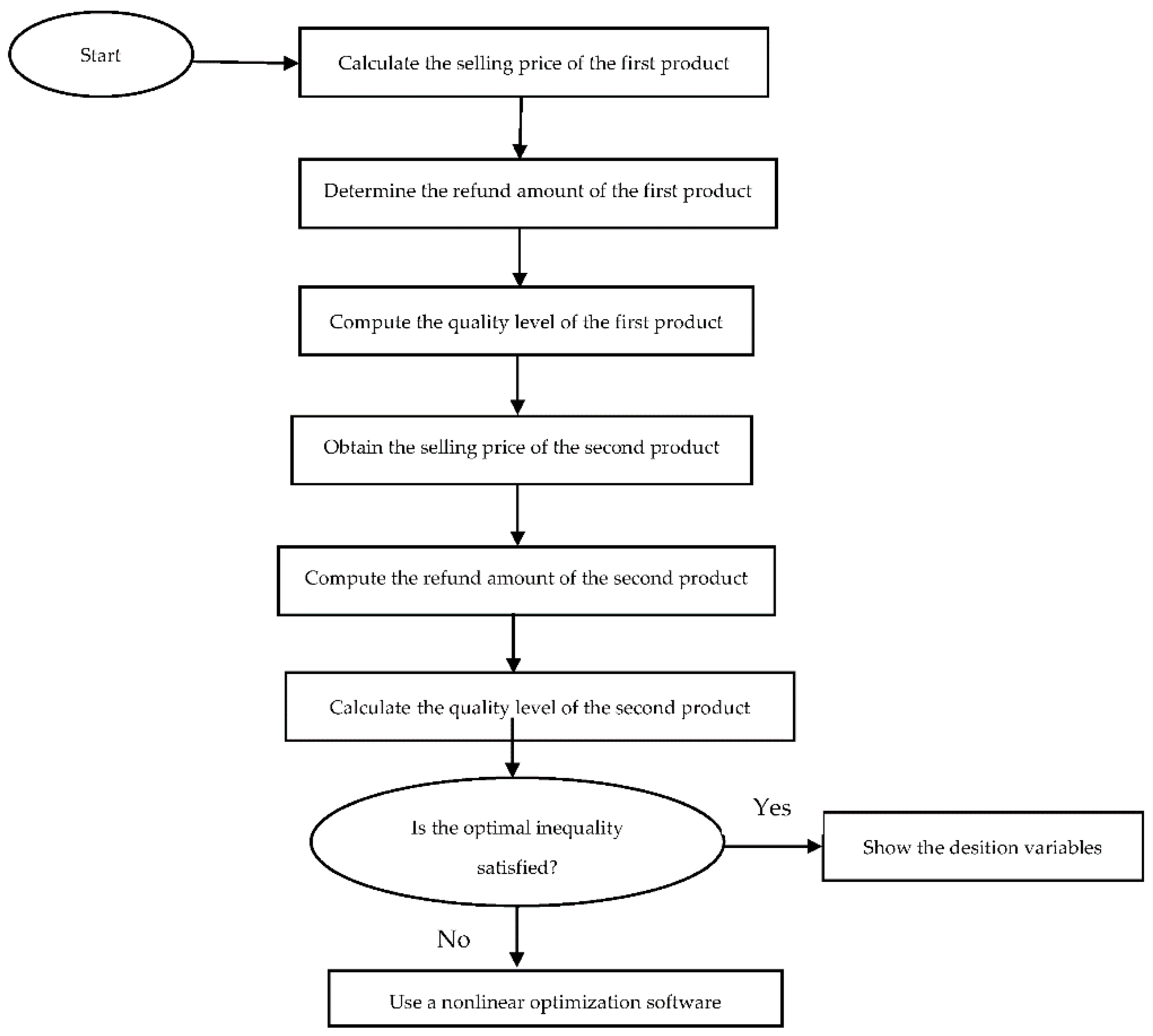
6. Solution Algorithm
7. Illustrative Example
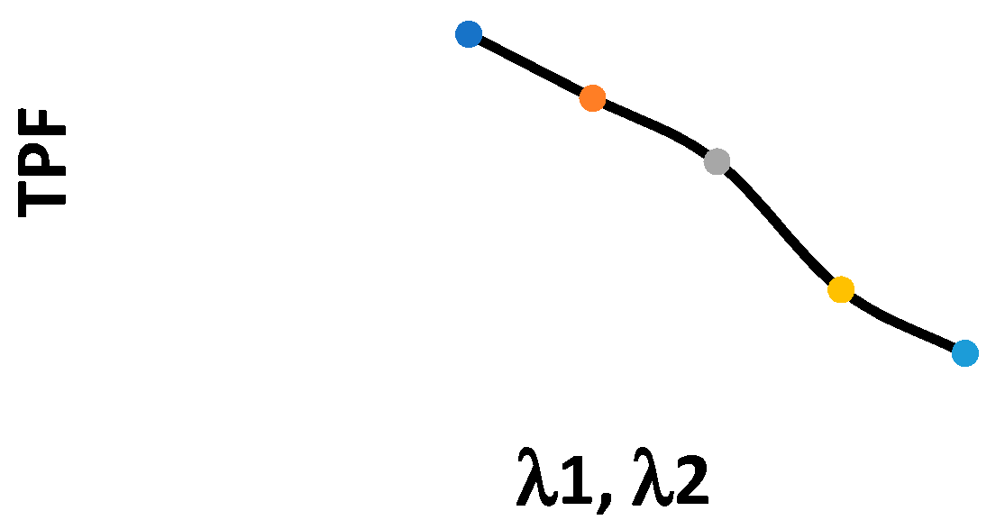
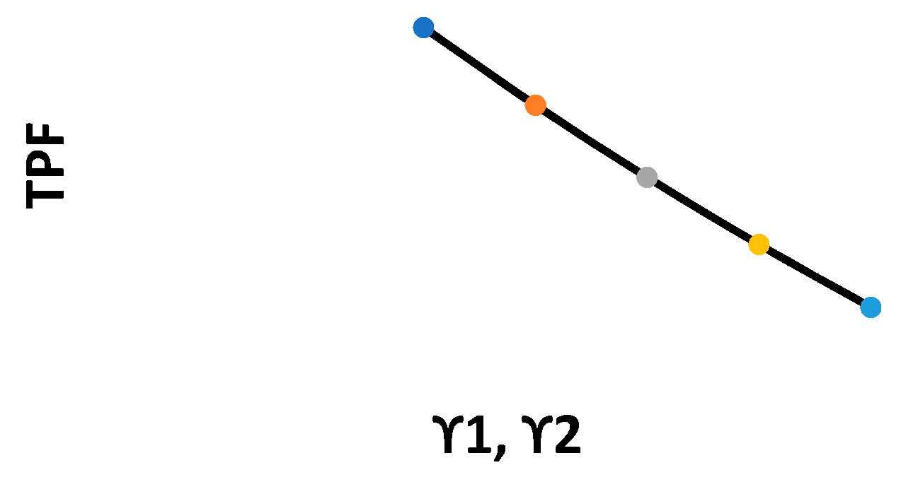
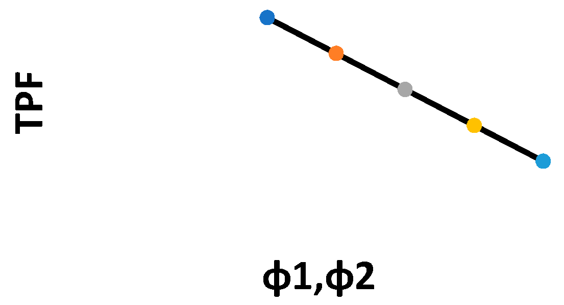
7.1. Sensitivity Analysis
- For the first product, optimal values of the decision variables are highly sensitive to an increase in α1;
- is highly sensitive to a decrease in , and is highly sensitive to a decrease in ;
- Optimal values for decision variables are moderately sensitive to decreases in and ;
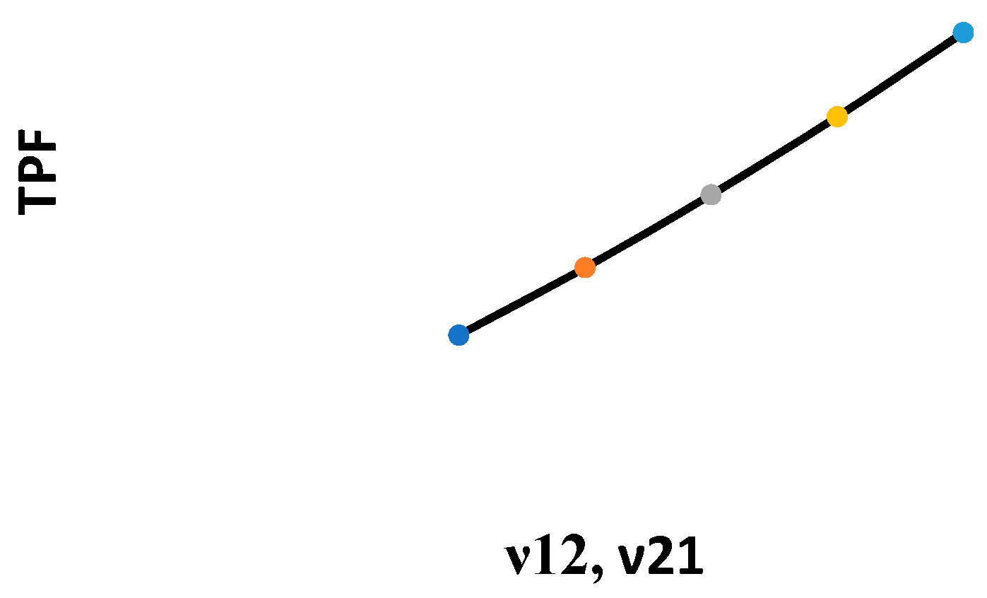
- is sensitive to an increase in , and is sensitive to an increase in ;
- Optimal values for decision variables are slightly sensitive to changes in and ;
- and are highly sensitive to a 40% decrease in parameter ;
- and are highly sensitive to a 40% decrease in parameter ;
- For the first product, optimal values of the decision variables are highly sensitive to a 40% decrease in parameter ;
- For the second product, optimal values of the decision variables are highly sensitive to a 40% decrease in parameter ;
- and are sensitive to a 40% increase in parameter ;
- and are sensitive to a 40% increase in parameter ;
- and are moderately sensitive to a 40 and 20% increase, respectively, parameter ;
- Change in the values of and does not have a significant effect on the optimal value of decision variables.
7.2. Managerial Insight
- This study filled an important research gap in presenting a comprehensive model for two complementary products in online selling where a return policy exists, by deciding on the selling price, quality level, and refund amount for returned products.
- As the potential market demand has a positive effect on the online distributor’s profit, the managers should try to expand the target market of their products by applying appropriate marketing policies.
- Managers of two complementary products should spend more on the refund of returned products when the sensitivity of demand to refund amount is high. By applying this strategy, the demand will increase, and the online distributor can increase the selling price and quality.
- With an increasing sensitivity of returned quantity with respect to product quality, the online distributor should provide products with a higher quality and, correspondingly, retain the price and the refund amount.
- Managers should decrease the price of the first (or second) product by increasing the sensitivity of its demand to price. In contrast, they are advised to increase the price of the second (or first) product.
- The negative effect of the quality cost parameter on profit implies that managers should reduce the quality and keep the refund on returned products unchanged. In other words, they should take the position of “low quality and low price”.
- When customers are less sensitive to a return policy, they will pay more attention to quality. Thus, managers should seek a lenient return policy, such as increasing the quality and refund on returned products.
- The proposed model is a proper starting point to present a new model that considers other marketing variables, such as advertising.
8. Conclusions
Author Contributions
Funding
Institutional Review Board Statement
Informed Consent Statement
Data Availability Statement
Conflicts of Interest
Appendix A. A Proof of the Concavity of the Profit Functions for the Both Products
Appendix B. A Proof of the Concavity of the Total Profit Functions with Respect to Hessian Matrix
Appendix C. Deriving the Optimal Decision Variables
References
- Chopra, S.; Meindl, P. Strategy, Planning, and Operation. In Supply Chain Management; Pearson: New York, NY, USA, 2001. [Google Scholar]
- Reagan, C. That Sweater You Don’t Like Is a Trillion-Dollar Problem for Retailers. These Companies Want to Fix it. 2019. Available online: https://www.cnbc.com/2019/01/10/growing-online-sales-means-more-returns-and-trash-for-landfills.html (accessed on 21 April 2021).
- Son, J.; Kang, J.H.; Jang, S. The effects of out-of-stock, return, and cancellation amounts on the order amounts of an online retailer. Retail. Consum. Serv. 2019, 51, 421–427. [Google Scholar] [CrossRef]
- Suwelack, T.; Hogreve, J.; Hoyer, W.D. Understanding money-back guarantees: Cognitive, affective, and behavioral outcomes. J. Retail. 2011, 87, 462–478. [Google Scholar] [CrossRef]
- Wai, K.; Dastane, O.; Johari, Z.; Ismail, N.B. Perceived risk factors affecting consumers’ online shopping behavior. J. Asian Financ. Econ. Bus. 2019, 6, 246–260. [Google Scholar]
- Khouja, M.; Ajjan, H.; Liu, X. The effect of return and price adjustment policies on a retailer’s performance. Eur. J. Oper. Res. 2019, 276, 466–482. [Google Scholar] [CrossRef]
- Pourhejazy, P. Destruction Decisions for Managing Excess Inventory in E-Commerce Logistics. Sustainability 2020, 12, 8365. [Google Scholar] [CrossRef]
- Mollenkopf, D.A.; Rabinovich, E.; Laseter, T.M.; Boyer, K.K. Managing internet product returns: A focus on effective service operations. Decis. Sci. 2007, 38, 215–250. [Google Scholar] [CrossRef]
- Tariq, A.; Bashir, B.; Adnan Shad, M. Factors affecting online shopping behavior of consumers in Pakistan. J. Mark. Consum. Res. 2016, 19, 95. [Google Scholar]
- Pei, Z.; Paswan, A. Consumers’ Legitimate and Opportunistic Product Return Behaviors in Online Shopping. J. Electron. Commer. Res. 2018, 19, 301–319. [Google Scholar]
- Cao, K.; Xu, Y.; Wang, J. Should firms provide online return service for remanufactured products? J. Clean. Prod. 2020, 272, 122641. [Google Scholar] [CrossRef]
- Fan, Z.P.; Chen, Z. When should the e-tailer offer complimentary return-freight insurance? Int. J. Prod. Econ. 2020, 230, 107890. [Google Scholar] [CrossRef]
- Kirmani, A.; Roa, A.R. No pain, no gain: A critical review of the literature on signaling unobservable quality. J. Mark. 2000, 64, 66–79. [Google Scholar] [CrossRef]
- Whitefield, R.I.; Duffy, A.H.B. Extended revenue forecasting within a service industry. Int. J. Prod. Econ. 2012, 141, 505–518. [Google Scholar] [CrossRef]
- Rabinovich, E.; Maltz, A.; Sinha, R.K. Assessing markups, service quality, and product attributes in music CDs’ internet retailing. Prod. Oper. Manag. 2008, 17, 320–337. [Google Scholar] [CrossRef]
- Li, Y.; Lei, X.; Li, D. Examining relationships between the return policy, product quality, and pricing strategy in online direct selling. Int. J. Prod. Econ. 2013, 144, 451–460. [Google Scholar] [CrossRef]
- Yoo, S.H. Product quality and return policy in a supply chain under risk aversion of a supplier. Int. J. Prod. Econ. 2014, 154, 146–155. [Google Scholar] [CrossRef]
- Li, G.; Li, L.; Sethi, S.P.; Guan, X. Return strategy and pricing in a dual-channel supply chain. Int. J. Prod. Econ. 2019, 215, 153–164. [Google Scholar] [CrossRef]
- Zhao, J.; Hou, X.; Guo, Y.; Wei, J. Pricing policies for complementary products in a dual-channel supply chain. Appl. Math. Model. 2017, 49, 437–451. [Google Scholar] [CrossRef]
- Pasternack, B.A. Optimal pricing and return polices for perishable commodities. Mark. Sci. 1985, 4, 166–176. [Google Scholar] [CrossRef]
- Kandel, E. The right to return. J. Law Econ. 1996, 39, 329–356. [Google Scholar] [CrossRef]
- Emmons, H.; Gilbert, S.M. Note: The role of returns policies in pricing and inventory decisions for catalogue goods. Manag. Sci. 1998, 44, 276–283. [Google Scholar] [CrossRef]
- Lau, H.S.; Lau, A.H.L. Manufacturer’s pricing strategy and return policy for a single-period commodity. Eur. J. Oper. Res. 1999, 116, 291–304. [Google Scholar] [CrossRef]
- Webster, S.; Weng, Z.K. A risk free perishable item returns policy. Manuf. Serv. Oper. Manag. 2000, 2, 100–106. [Google Scholar] [CrossRef]
- Yao, D.Q.; Yue, X.; Wang, X.; Liu, J.J. The impact of information sharing on a return policy with the addition of a direct channel. Int. J. Prod. Econ. 2005, 97, 196–209. [Google Scholar] [CrossRef]
- Ringbom, S.; Oz, S. Advance booking, cancellations, and partial refunds. Econ. Bull. 2004, 13, 1–7. [Google Scholar]
- Mukhopadhyay, S.K.; Setaputra, R. A dynamic model for optimal design quality and return policies. Eur. J. Oper. Res. 2007, 180, 1144–1154. [Google Scholar] [CrossRef]
- Yue, X.; Raghunathan, S. The impacts of the full return policy on a supply chain with information asymmetry. Eur. J. Oper. Res. 2007, 180, 630–647. [Google Scholar] [CrossRef]
- Yao, Z.; Leung, S.C.H.; Lai, K.K. Analysis of the impact of price-sensitivity factors on the return policy in coordinating supply chain. Eur. J. Oper. Res. 2008, 187, 275–282. [Google Scholar] [CrossRef]
- Yu, C.C.; Wang, C.S. A hybrid mining approach for optimizing return policies in e-retailing. Expert Syst. Appl. 2008, 35, 1575–1582. [Google Scholar] [CrossRef]
- Su, X. Consumer returns policies and supply chain performance. Int. J. Adv. Oper. Manag. 2009, 11, 595–612. [Google Scholar] [CrossRef]
- Chen, J.; Bell, P.C. The impact of customer returns on pricing and order decisions. Eur. J. Oper. Res. 2009, 195, 280–295. [Google Scholar] [CrossRef]
- Bonifield, C.; Cole, C.; Schultz, R.L. Product returns on the internet: A case of mixed signals? J. Bus. Res. 2010, 63, 1058–1065. [Google Scholar] [CrossRef]
- Xiao, T.; Shi, K.; Yang, D. Coordination of a supply chain with consumer return under demand uncertainty. Int. J. Prod. Econ. 2010, 124, 171–180. [Google Scholar] [CrossRef]
- Chen, J.; Bell, P.C. Coordinating a decentralized supply chain with customer returns and price-dependent stochastic demand using a buyback policy. Eur. J. Oper. Res. 2011, 212, 293–300. [Google Scholar] [CrossRef]
- Ai, X.; Chen, J.; Zhao, H.; Tang, X. Competition among supply chains: Implications of full returns policy. Int. J. Prod. Econ. 2012, 139, 257–265. [Google Scholar] [CrossRef]
- Chen, J.; Grewal, R. Competing in a supply chain via full-refund and no–refund customer returns policies. Int. J. Prod. Econ. 2013, 146, 246–258. [Google Scholar] [CrossRef]
- Liu, J.; Mantin, B.; Wang, H. Supply chain coordination with customer returns and refund-dependent demand. Int. J. Prod. Econ. 2013, 148, 81–89. [Google Scholar] [CrossRef]
- Yoo, S.H.; Kim, D.; Park, M.S. Pricing and return policy under various supply contracts in a closed-loop supply chain. Int. J. Prod. Res. 2015, 53, 106–126. [Google Scholar] [CrossRef]
- Giri, B.C.; Bardhan, S. Coordinating a supply chain under uncertain demand and random yield in presence of supply disruption. Int. J. Prod. Res. 2015, 53, 5070–5084. [Google Scholar] [CrossRef]
- Heydaryan, H.; Taleizadeh, A.A. Pricing strategy, return policy and coordination in a two-stage supply chain. Int. J. System Sci. Oper. Logis. 2017, 4, 384–391. [Google Scholar] [CrossRef]
- Hu, X.; Wan, Z.; Murthy, N.N. Dynamic pricing of limited inventories with product returns. Manu. Serv. Oper. Manag. 2019, 21, 501–518. [Google Scholar] [CrossRef]
- Noori-daryan, M.; Taleizadeh, A.A. Optimizing pricing and ordering strategies in a three-level supply chain under return policy. J. Ind. Eng. Int. 2019, 15, 73–80. [Google Scholar] [CrossRef][Green Version]
- Ren, M.; Liu, J.; Feng, S.; Yang, A. Pricing and return strategy of online retailers based on return insurance. Retail. Consum. Serv. 2021, 59, 102350. [Google Scholar] [CrossRef]
- Yue, X.; Mukhopadhyay, S.; Zhu, X. A Bertrand model of pricing of complementary goods under information asymmetry. J. Bus. Res. 2006, 59, 1182–1192. [Google Scholar] [CrossRef]
- Bilotkach, V. Quality coordination and complementary products. Appl. Econ. 2010, 42, 1875–1888. [Google Scholar] [CrossRef]
- Mukhopadhyay, S.K.; Yue, X.H.; Zhu, X.W. A Stackelberg model of pricing of complementary goods under information asymmetry. Int. J. Prod. Econ. 2011, 134, 424–433. [Google Scholar] [CrossRef]
- Yan, R.; Bandyopadhyay, S. The profit benefits of bundle pricing of complementary products. J. Retail. Consum. Serv. 2011, 18, 355–361. [Google Scholar] [CrossRef]
- Wei, J.; Zhao, J.; Li, Y. Pricing decisions for complementary products with firms’ different market powers. Eur. J. Oper. Res. 2013, 224, 507–519. [Google Scholar] [CrossRef]
- Wei, J.; Zhao, J.; Li, Y. Price and warranty period decisions for complementary products with horizontal firms’ cooperation/noncooperation strategies. J. Clean. Prod. 2015, 105, 86–102. [Google Scholar] [CrossRef]
- Taleizadeh, A.A.; Charmchi, M. Optimal advertising and pricing decisions for complementary products. J. Ind. Eng. Int. 2015, 11, 111–117. [Google Scholar] [CrossRef]
- Dehghanbaghi, N.; Sajadieh, M.S. Joint optimization of production, transportation and pricing policies of complementary products in a supply chain. Comput. Ind. Eng. 2017, 107, 150–157. [Google Scholar] [CrossRef]
- Wang, L.; Song, H.; Wang, Y. Pricing and service decisions of complementary products in a dual-channel supply chain. Comput. Ind. Eng. 2017, 105, 223–233. [Google Scholar] [CrossRef]
- Taleizadeh, A.A.; Babaei, M.S.; Sana, S.S.; Sarkar, B. Pricing decision within an inventory model for complementary and substitutable products. Mathematics 2019, 7, 568. [Google Scholar] [CrossRef]
- Giri, R.N.; Mondal, S.K.; Maiti, M. Bundle pricing strategies for two complementary products with different channel powers. Ann. Oper. Res. 2020, 287, 701–725. [Google Scholar] [CrossRef]
- Ren, D.; Lan, Y.; Shang, C.; Wang, J.; Xue, C. Impacts of trade credit on pricing decisions of complementary products. Comput. Ind. Eng. 2020, 146, 106580. [Google Scholar] [CrossRef]
- Shan, H.; Zhang, C.; Wei, G. Bundling or Unbundling? Pricing Strategy for Complementary Products in a Green Supply Chain. Sustainability 2020, 12, 1331. [Google Scholar] [CrossRef]
- Coughlan, A.T. Distribution channel choice in a market with complementary goods. Int. J. Res. Mark. 1987, 4, 85–97. [Google Scholar] [CrossRef]
- Balachander, S. Warranty signaling and reputation. Manag. Sci. 2001, 47, 1282–1289. [Google Scholar] [CrossRef]
- Taleizadeh, A.A.; Kalantary, S.S.; Cárdenas-Barrón, L.E. Pricing and Lot sizing for an EPQ Inventory Model with Rework and Multiple Shipments. TOP 2016, 24, 143–155. [Google Scholar] [CrossRef]
- Taleizadeh, A.A.; Noori-Daryan, M. Pricing, Replenishments and Production Policies in a Supply Chain of Pharmacological Product with Rework Process: A Game Theoretic Approach. Oper. Res. Int. J. 2016, 16, 89–115. [Google Scholar] [CrossRef]
- Taleizadeh, A.A.; Alizadeh-Pasban, N.; Sarker, B.R. Coordinated contracts in a two-level green supply chain considering pricing strategy. Comput. Ind. Eng. 2018, 124, 249–275. [Google Scholar] [CrossRef]
- Taleizadeh, A.A. Lot sizing model with advance payment and disruption in supply under planned partial backordering. Int. Trans. Oper. Res. 2017, 24, 783–800. [Google Scholar] [CrossRef]
- Lashgari, M.; Taleizadeh, A.A.; Ahmadi, A. Partial up-stream advanced payment and partial down-stream delayed payment in a three-level supply chain. Ann. Oper. Res. 2016, 238, 329–354. [Google Scholar] [CrossRef]
- Taleizadeh, A.A.; Niaki, S.T.A.; Hosseini, V. Optimizing Multi Product Multi Constraints Bi-objective Newsboy Problem with discount by Hybrid Method of Goal Programming and Genetic Algorithm. Eng. Optim. 2009, 41, 437–457. [Google Scholar] [CrossRef]


| Symbol | Definition |
|---|---|
| i | Set of products (for i = 1,2) |
| Di | The demand function of the ith product (units) |
| αi | The potential market demand for the ith product (units) |
| The sensitivity of the ith product demand with respect to the selling price of the (3-i)th product | |
| The sensitivity of the ith product demand with respect to the return rate of the ith product | |
| The sensitivity of the ith product demand with respect to the return rate of the (3-i)th product | |
| The return quantity factor of the ith product that is not dependent on quality and return policy | |
| The sensitivity of the ith product returns quantity with respect to its quality level | |
| The total quality improvement cost of the ith product (USD) | |
| The returned quantity of the ith product (unit) | |
| The unit producing cost of the ith product (USD/unit) | |
| The return quantity of the ith product affected by the return quantity of the (3-i)th product | |
| TPF | The total profit function (USD) |
| Symbol | Definition |
|---|---|
| The selling price of the ith product (USD/unit) | |
| The refund amount on the return of the ith product (USD/unit) | |
| ) |
| Percentage | New Value of Decision Variable | Change Percentage of Decision Variable | TPF | ||||||||||||
|---|---|---|---|---|---|---|---|---|---|---|---|---|---|---|---|
| = 1400 | −40% | 840 | 93.9 | 920.3 | 0.17 | 0.51 | 60.7 | 155 | −84% | 36% | −69% | 4% | −69% | 3% | 709.140 |
| −20% | 1120 | 342.9 | 797.6 | 0.36 | 0.50 | 129.2 | 152.4 | −42% | 18% | −35% | 2% | −34% | 1% | 766.960 | |
| 20% | 1680 | 840.9 | 552.2 | 0.76 | 0.49 | 266.1 | 147.3 | 42% | −18% | 35% | 0% | 34% | −1% | 1091.800 | |
| 40% | 1960 | 1090 | 429.5 | 0.95 | 0.48 | 334.5 | 144.7 | 84% | −36% | 69% | −2% | 69% | −3% | 1358.700 | |
| = 1500 | −40% | 900 | 855 | 161.9 | 0.72 | 0.28 | 254.7 | 84.2 | 44% | −76% | 28% | −42% | 28% | −43% | 651.170 |
| −20% | 1200 | 723.5 | 418.4 | 0.64 | 0.39 | 226.1 | 117 | 22% | −38% | 14% | −20% | 14% | −21% | 734.310 | |
| 20% | 1800 | 460.4 | 931.4 | 0.48 | 0.60 | 169.1 | 182.7 | −22% | 38% | −14% | 22% | −14% | 21% | 1131.700 | |
| 40% | 2100 | 328.9 | 1187.9 | 0.40 | 0.71 | 140.6 | 215.6 | −44% | 76% | −28% | 44% | −28% | 43% | 1446 | |
| = 70 | −40% | 42 | 592 | 674.9 | 0.94 | 0.49 | 197.8 | 149.9 | 0.01% | 0% | 67% | 0% | 0.55% | 0% | 894.510 |
| −20% | 56 | 591.9 | 674.9 | 0.70 | 0.49 | 197.7 | 149.9 | 0% | 0% | 25% | 0% | 0.50% | 0% | 894.500 | |
| 20% | 84 | 591.9 | 674.9 | 0.47 | 0.49 | 197.6 | 149.9 | 0% | 0% | −16% | 0% | 0% | 0% | 894.490 | |
| 40% | 98 | 591.9 | 674.9 | 0.40 | 0.49 | 197.6 | 149.9 | 0% | 0% | −28% | 0% | 0% | 0% | 894.490 | |
| = 60 | −40% | 36 | 591.9 | 674.9 | 0.56 | 0.83 | 197.6 | 150 | 0% | 0% | 0% | 69% | 0% | 0.06% | 894.510 |
| −20% | 48 | 591.9 | 674.9 | 0.56 | 0.62 | 197.6 | 149.9 | 0% | 0% | 0% | 26% | 0% | 0% | 894.500 | |
| 20% | 72 | 591.6 | 674.9 | 0.56 | 0.41 | 197.6 | 149.8 | −0.05% | 0% | 0% | −16% | 0% | −0.06% | 894.490 | |
| 40% | 84 | 591.6 | 674.9 | 0.56 | 0.35 | 197.6 | 149.8 | −0.05% | 0% | 0% | −28% | 0% | −0.06% | 894.490 | |
| = 0.4 | −40% | 0.24 | 648.5 | 712.3 | 0.61 | 0.53 | 215.8 | 160 | 9% | 5% | 8% | 8% | 9% | 6% | 961.840 |
| −20% | 0.32 | 619.8 | 692.3 | 0.59 | 0.51 | 206.5 | 154.7 | 4% | 2% | 5% | 4% | 4% | 3% | 926.940 | |
| 20% | 0.48 | 564.4 | 660.1 | 0.53 | 0.48 | 188.9 | 145.5 | −4% | −2% | −5% | −2% | −4% | −2% | 864.290 | |
| 40% | 0.56 | 536.6 | 648.3 | 0.51 | 0.47 | 180.3 | 141.6 | −9% | −3% | −8% | −4% | −8% | −5% | 836.120 | |
| = 0.4 | −40% | 0.24 | 646.5 | 714.1 | 0.61 | 0.53 | 215.3 | 160.2 | 9% | 5% | 8% | 8% | 8% | 6% | 961.740 |
| −20% | 0.32 | 618.7 | 693.3 | 0.58 | 0.51 | 206.3 | 154.8 | 4% | 2% | 3% | 4% | 4% | 3% | 926.900 | |
| 20% | 0.48 | 565.7 | 658.9 | 0.54 | 0.48 | 189.3 | 145.4 | −4% | −2% | −3% | −2% | −4% | −3% | 864.300 | |
| 40% | 0.56 | 539.6 | 645.5 | 0.51 | 0.47 | 181.1 | 141.3 | −8% | −4% | −8% | −4% | −8% | −5% | 836.120 | |
| = 0.4 | −40% | 0.24 | 591.9 | 674.9 | 0.33 | 0.49 | 197.5 | 149.9 | 0% | 0% | −41% | 0% | −0.05% | 0% | 894.488 |
| −20% | 0.32 | 591.9 | 674.9 | 0.45 | 0.49 | 197.5 | 149.9 | 0% | 0% | −19% | 0% | −0.05% | 0% | 894.490 | |
| 20% | 0.48 | 591.9 | 674.9 | 0.67 | 0.49 | 197.7 | 149.9 | 0% | 0% | 19% | 0% | 0.05% | 0% | 894.510 | |
| 40% | 0.56 | 591.9 | 674.9 | 0.79 | 0.49 | 197.9 | 149.9 | 0.01% | 0% | 41% | 0% | 0.15% | 0% | 894.520 | |
| = 0.4 | −40% | 0.24 | 591.9 | 674.9 | 0.56 | 0.29 | 197.6 | 149.8 | 0% | 0% | 0% | −40% | 0% | −0.06% | 894.480 |
| −20% | 0.32 | 591.9 | 674.9 | 0.56 | 0.39 | 197.6 | 149.8 | 0% | 0% | 0% | −20% | 0% | −0.06% | 894.490 | |
| 20% | 0.48 | 591.9 | 674.9 | 0.56 | 0.59 | 197.6 | 149.9 | 0% | 0% | 0% | 20% | 0% | 0% | 894.500 | |
| 40% | 0.56 | 591.9 | 674.9 | 0.56 | 0.70 | 197.6 | 150 | 0% | 0% | 0% | 42% | 0% | 0.06% | 894.510 | |
| = 0.1 | −40% | 0.06 | 592 | 674.9 | 0.56 | 0.49 | 197.8 | 149.9 | 0% | 0% | 0% | 0% | 0.05% | 0% | 894.525 |
| −20% | 0.08 | 591.9 | 674.9 | 0.56 | 0.49 | 197.8 | 149.9 | 0% | 0% | 0% | 0% | 0.05% | 0% | 894.521 | |
| 20% | 0.12 | 591.9 | 674.9 | 0.56 | 0.49 | 197.7 | 149.9 | 0% | 0% | 0% | 0% | 0% | 0% | 894.513 | |
| 40% | 0.14 | 591.9 | 674.9 | 0.56 | 0.49 | 197.7 | 149.9 | 0% | 0% | 0% | 0% | 0% | 0% | 894.509 | |
| = 0.1 | −40% | 0.06 | 591.9 | 674.9 | 0.56 | 0.50 | 197.8 | 150 | 0% | 0% | 0% | 0% | 0% | 0% | 894.538 |
| −20% | 0.08 | 591.9 | 674.9 | 0.56 | 0.50 | 197.8 | 150 | 0% | 0% | 0% | 0% | 0% | 0% | 894.536 | |
| 20% | 0.12 | 591.9 | 674.9 | 0.56 | 0.49 | 197.7 | 149.9 | 0% | 0% | 0% | −2% | −0.05% | −0.06% | 894.530 | |
| 40% | 0.14 | 591.9 | 674.9 | 0.56 | 0.49 | 197.7 | 149.9 | 0% | 0% | 0% | −2% | −0.05% | −0.06% | 894.526 | |
| = 0.5 | −40% | 0.3 | 625.8 | 662.6 | 0.98 | 0.50 | 345.5 | 150.2 | 5% | −1% | 75% | 2% | 74% | 0.2% | 908.070 |
| −20% | 0.4 | 604.2 | 670.4 | 0.71 | 0.50 | 251.4 | 150 | 2% | −0.66% | 26% | 2% | 27% | 0.06% | 899.440 | |
| 20% | 0.6 | 583.9 | 677.8 | 0.46 | 0.49 | 162.8 | 149.8 | −1% | 0.42% | −17% | 0% | −17% | −0.06% | 891.300 | |
| 40% | 0.7 | 578.3 | 679.8 | 0.39 | 0.49 | 138.4 | 149.7 | −2% | 0.72% | −30% | 0% | −29% | −0.13% | 889.060 | |
| = 0.6 | −40% | 0.36 | 592 | 687.8 | 0.56 | 0.84 | 198.2 | 253.5 | 0.01% | 1% | 0% | 71% | 0.3% | 69% | 903.590 |
| −20% | 0.48 | 592 | 679.7 | 0.56 | 0.62 | 197.8 | 188.4 | 0.01% | 0.71% | 0% | 26% | 0.1% | 25% | 897.870 | |
| 20% | 0.72 | 591.9 | 671.7 | 0.56 | 0.41 | 197.5 | 124.4 | 0% | −0.47% | 0% | −16% | −0.05% | −17% | 892.270 | |
| 40% | 0.84 | 591.9 | 669.5 | 0.56 | 0.35 | 197.4 | 106.4 | 0% | −0.8%1% | 0% | −28% | 0.1% | −29% | 890.680 | |
| = 0.8 | −40% | 0.48 | 1367.5 | 292.8 | 1 | 0.47 | 410.8 | 141.9 | 100% | −56% | 78% | −4% | 100% | −5% | 1148.700 |
| −20% | 0.64 | 825.4 | 559.8 | 0.74 | 0.49 | 261.8 | 147.5 | 39% | −17% | 32% | 0% | 32% | −1% | 971.030 | |
| 20% | 0.96 | 461.9 | 739 | 0.46 | 0.50 | 161.9 | 151.2 | −21% | 9% | −17% | 2% | −18% | 0.86% | 851.880 | |
| 40% | 1.12 | 379 | 779.8 | 0.39 | 0.50 | 139.1 | 152.1 | −35% | 15% | −30% | 2% | −29% | 1% | 824.720 | |
| = 0.8 | −40% | 0.48 | 177.4 | 1483.2 | 0.30 | 0.84 | 107.8 | 253.4 | −70% | 100% | −46% | 71% | −45% | 69% | 1210.600 |
| −20% | 0.64 | 462.7 | 926.8 | 0.48 | 0.60 | 169.6 | 182.1 | −21% | 37% | −14% | 22% | −14% | 21% | 992.920 | |
| 20% | 0.96 | 665.6 | 531.2 | 0.61 | 0.43 | 213.6 | 131.5 | 12% | −21% | 8% | −12% | 8% | −12% | 838.400 | |
| 40% | 1.12 | 713.2 | 438.3 | 0.63 | 0.39 | 223.9 | 119.6 | 20% | −35% | 12% | −20% | 13% | −20% | 802.160 | |
| = 0.3 | −40% | 0.18 | 562.5 | 687.6 | 0.35 | 0.50 | 123.3 | 152.6 | −4% | 1% | −37% | 2% | −37% | 1% | 884.230 |
| −20% | 0.24 | 575.1 | 682.3 | 0.45 | 0.50 | 159.1 | 151.3 | −2% | 1% | −19% | 2% | −19% | 0.93% | 888.680 | |
| 20% | 0.36 | 613.6 | 665.2 | 0.68 | 0.49 | 239.8 | 148.3 | 3% | −1% | 21% | 0% | 21% | −1% | 901.920 | |
| 40% | 0.42 | 641.1 | 652.7 | 0.81 | 0.48 | 286.8 | 146.5 | 8% | −3% | 44% | −2% | 45% | −2% | 911.280 | |
| = 0.2 | −40% | 0.12 | 596.2 | 662 | 0.57 | 0.32 | 201 | 104.8 | 0.72% | −1% | 1% | −30% | 1% | −30% | 888.370 |
| −20% | 0.16 | 594.4 | 667.6 | 0.56 | 0.42 | 199.4 | 127 | 0.42% | −1% | 0% | −14% | 0.91% | −15% | 891.130 | |
| 20% | 0.24 | 588.6 | 683.8 | 0.55 | 0.57 | 195.7 | 173.4 | −0.55% | 1% | −1% | 16% | −0.96% | 15% | 898.530 | |
| 40% | 0.28 | 584.4 | 694.4 | 0.55 | 0.66 | 193.4 | 198 | −1% | 2% | −1% | 34% | −2% | 32% | 903.260 | |
| = 0.1 | −40% | 0.06 | 587.5 | 674.6 | 0.56 | 0.43 | 197.5 | 130.3 | −0.74% | −0.04% | 0% | −12% | −0.05% | −13% | 891.500 |
| −20% | 0.08 | 589.6 | 674.8 | 0.56 | 0.46 | 197.5 | 140 | −0.38% | −0.01% | 0% | −6% | −0.05% | −6% | 892.940 | |
| 20% | 0.12 | 594.6 | 674.8 | 0.56 | 0.53 | 197.8 | 159.8 | 0.45% | −0.01% | 0% | 8% | 0.05% | 6% | 896.170 | |
| 40% | 0.14 | 597.7 | 674.5 | 0.56 | 0.56 | 198.1 | 169.8 | 0.97% | −0.05% | 0% | 14% | 0.25% | 13% | 897.970 | |
| = 0.05 | −40% | 0.03 | 590.3 | 673 | 0.52 | 0.50 | 183.9 | 150 | −0.27% | −0.28% | −7% | 2% | −6% | 0.06% | 892.090 |
| −20% | 0.04 | 591.1 | 673.9 | 0.54 | 0.49 | 190.7 | 149.9 | −0.13% | −0.14% | −3% | 0% | −3% | 0% | 893.270 | |
| 20% | 0.06 | 592.6 | 676 | 0.58 | 0.49 | 204.5 | 149.8 | 0.11% | 0.16% | 3% | 0% | 3% | −0.06% | 895.770 | |
| 40% | 0.07 | 593.3 | 677.2 | 0.60 | 0.49 | 211.4 | 149.8 | 0.23% | 0.34% | 7% | 0% | 6% | −0.06% | 897.100 | |
| = 0.1 | −40% | 0.06 | 592.9 | 674.5 | 0.57 | 0.50 | 202 | 150 | 0.16% | −0.05% | 1% | 2% | 2% | 0.06% | 895.330 |
| −20% | 0.08 | 592.4 | 674.7 | 0.57 | 0.50 | 199.8 | 150 | 0.08% | −0.02% | 1% | 2% | 1% | 0.06% | 894.910 | |
| 20% | 0.12 | 591.4 | 675.1 | 0.55 | 0.49 | 195.5 | 149.8 | −0.08% | 0.02% | −1% | 0% | −1% | −0.06% | 894.090 | |
| 40% | 0.14 | 590.9 | 675.2 | 0.55 | 0.49 | 193.3 | 149.7 | −0.16% | 0.04% | −1% | 0% | −2% | −0.13% | 893.680 | |
| = 0.1 | −40% | 0.06 | 592 | 675.3 | 0.56 | 0.51 | 197.9 | 153.6 | 0.01% | 0.05% | 0% | 4% | 0.15% | 2% | 895.200 |
| −20% | 0.08 | 591.9 | 675.1 | 0.56 | 0.50 | 197.8 | 151.7 | 0% | 0.02% | 0% | 2% | 0.10% | 1% | 894.850 | |
| 20% | 0.12 | 591.9 | 674.7 | 0.56 | 0.49 | 197.5 | 148 | 0% | −0.02% | 0% | 0% | −0.05% | −1% | 894.150 | |
| 40% | 0.14 | 591.9 | 674.4 | 0.56 | 0.48 | 197.4 | 146.1 | 0% | −0.07% | 0% | −2% | −0.10% | −2% | 893.810 | |
Publisher’s Note: MDPI stays neutral with regard to jurisdictional claims in published maps and institutional affiliations. |
© 2021 by the authors. Licensee MDPI, Basel, Switzerland. This article is an open access article distributed under the terms and conditions of the Creative Commons Attribution (CC BY) license (https://creativecommons.org/licenses/by/4.0/).
Share and Cite
Taleizadeh, A.A.; Beydokhti, S.R.; Cárdenas-Barrón, L.E.; Najafi-Ghobadi, S. Pricing of Complementary Products in Online Purchasing under Return Policy. J. Theor. Appl. Electron. Commer. Res. 2021, 16, 1718-1739. https://doi.org/10.3390/jtaer16050097
Taleizadeh AA, Beydokhti SR, Cárdenas-Barrón LE, Najafi-Ghobadi S. Pricing of Complementary Products in Online Purchasing under Return Policy. Journal of Theoretical and Applied Electronic Commerce Research. 2021; 16(5):1718-1739. https://doi.org/10.3390/jtaer16050097
Chicago/Turabian StyleTaleizadeh, Ata Allah, Shima Rezvan Beydokhti, Leopoldo Eduardo Cárdenas-Barrón, and Somayeh Najafi-Ghobadi. 2021. "Pricing of Complementary Products in Online Purchasing under Return Policy" Journal of Theoretical and Applied Electronic Commerce Research 16, no. 5: 1718-1739. https://doi.org/10.3390/jtaer16050097
APA StyleTaleizadeh, A. A., Beydokhti, S. R., Cárdenas-Barrón, L. E., & Najafi-Ghobadi, S. (2021). Pricing of Complementary Products in Online Purchasing under Return Policy. Journal of Theoretical and Applied Electronic Commerce Research, 16(5), 1718-1739. https://doi.org/10.3390/jtaer16050097