Parkinson’s Disease Tremor Detection in the Wild Using Wearable Accelerometers

 ,
,  , ,
, ,
Abstract
1. Introduction
2. Related Work
2.1. Feature Sets
2.2. Classification Algorithms
2.3. In-the-Wild Monitoring Systems
3. Methods
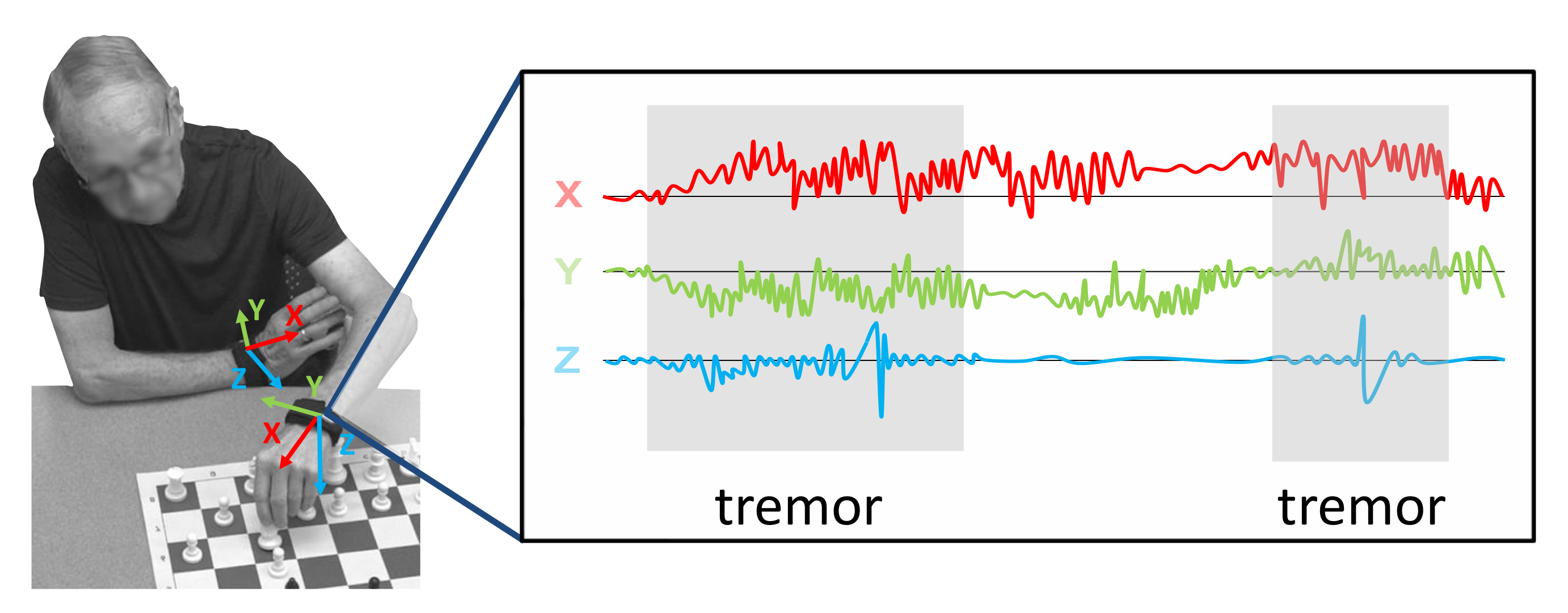
3.1. Data Collection
3.1.1. Laboratory Recordings (LAB)
3.1.2. In-the-Wild Recordings (WILD)
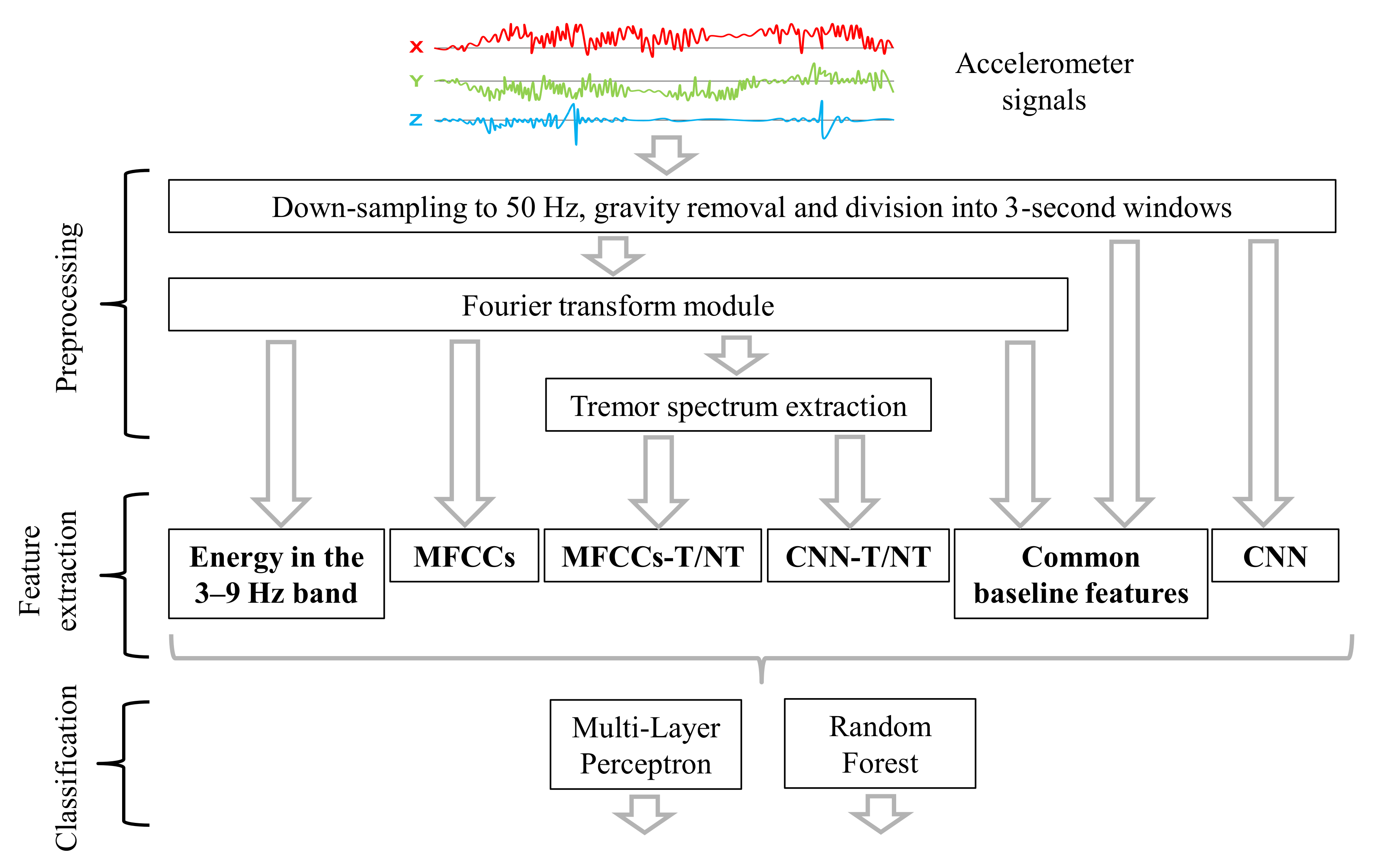
3.2. Preprocessing
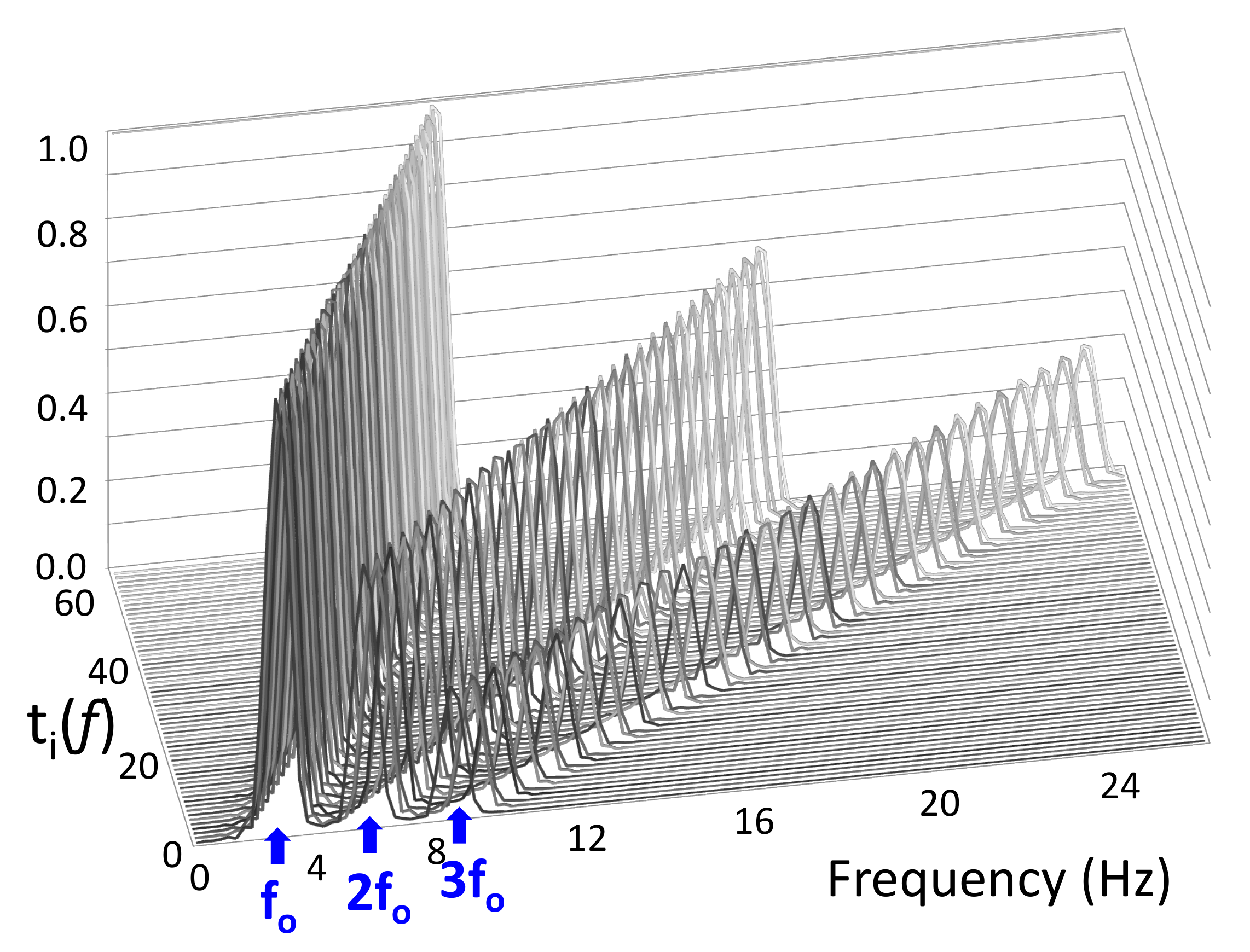
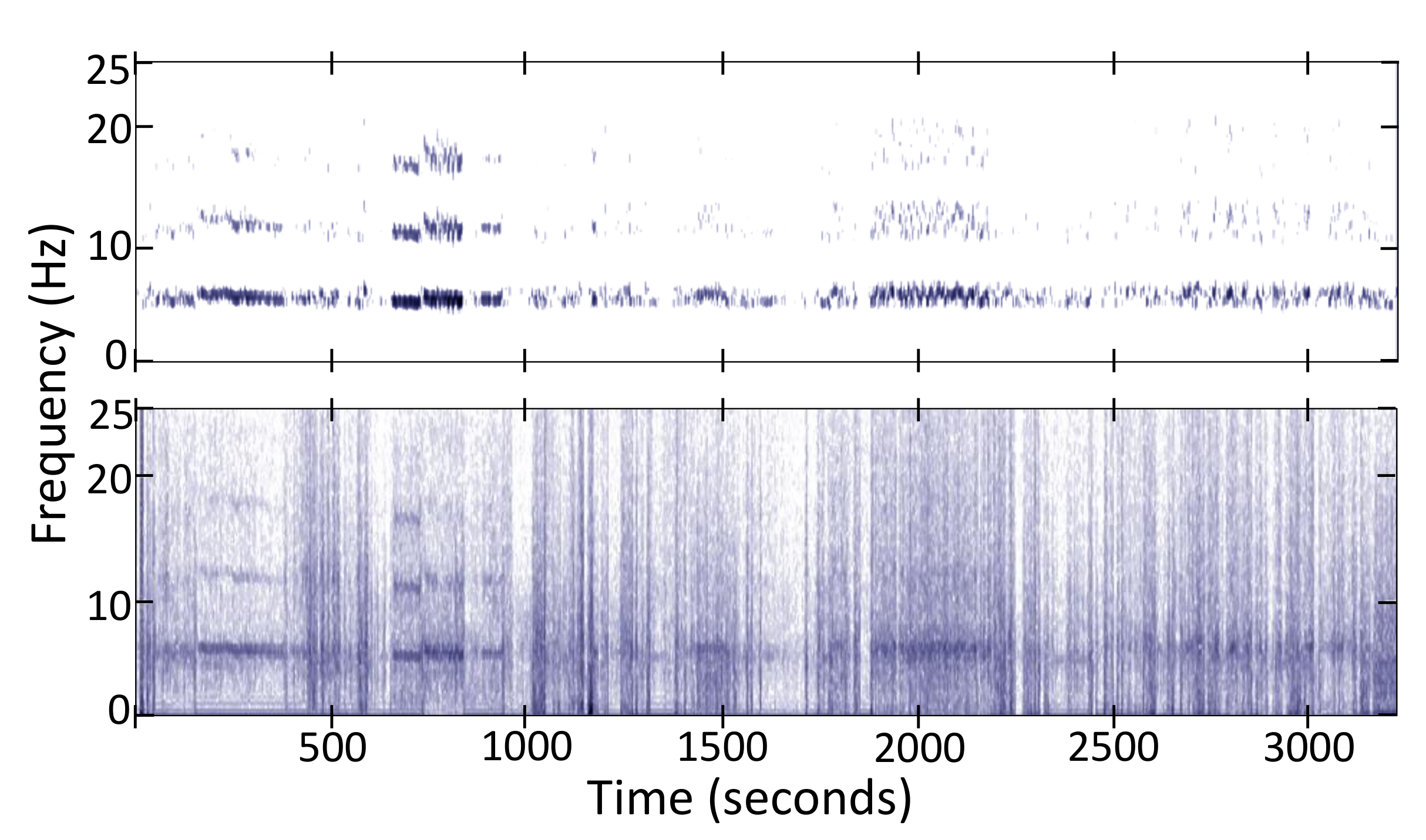
Non-Negative Tremor Factorization
3.3. Feature Extraction
3.3.1. Energy in the 3–9 Hz Band (Energy Threshold)
3.3.2. Welch’s One-Sided Power Spectral Density (PSD)
3.3.3. Common Baseline Features (Baseline)
3.3.4. Mel Frequency Cepstral Coefficients (MFCCs)
3.3.5. Mel Frequency Cepstral Coefficients after Tremor Spectrum Extraction (MFCCs-T/NT)
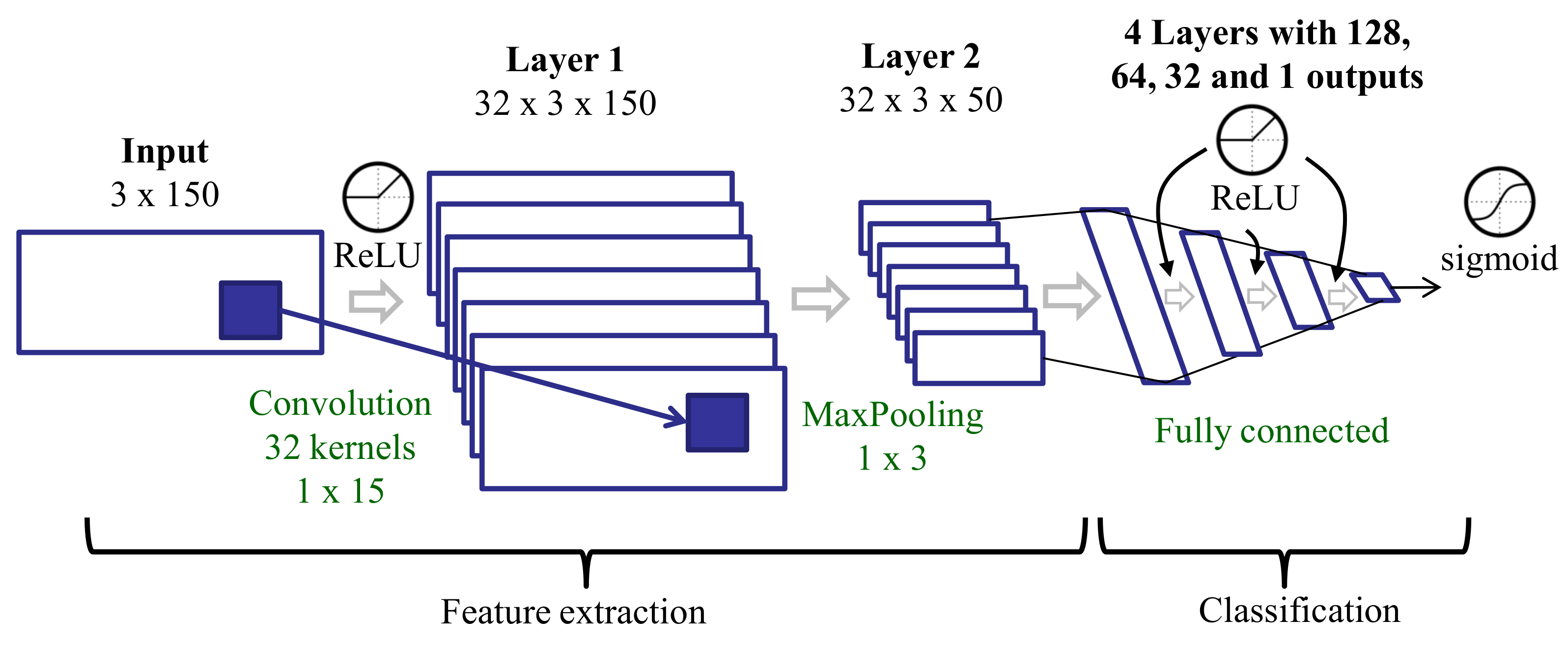
3.3.6. Features Learned with a CNN Trained on Raw Data (CNN)
3.3.7. Features Learned with a CNN Trained on Spectra after Tremor Spectrum Extraction (CNN-T/NT)
3.4. Classification Algorithms
3.4.1. Fully Supervised Learning
3.4.2. Weakly Supervised Learning
4. Experiments
- How well do our proposed feature sets and ML algorithms generalize to patients that are not in the training set?
- How does our best system (feature set + ML algorithm) compare to previous work?
- How well can an automatic method reproduce patient self-assessments of tremor, the current standard for in-home monitoring?
- How well can an automated system approximate the percentage of tremor time over long intervals (hours, days, or weeks)?
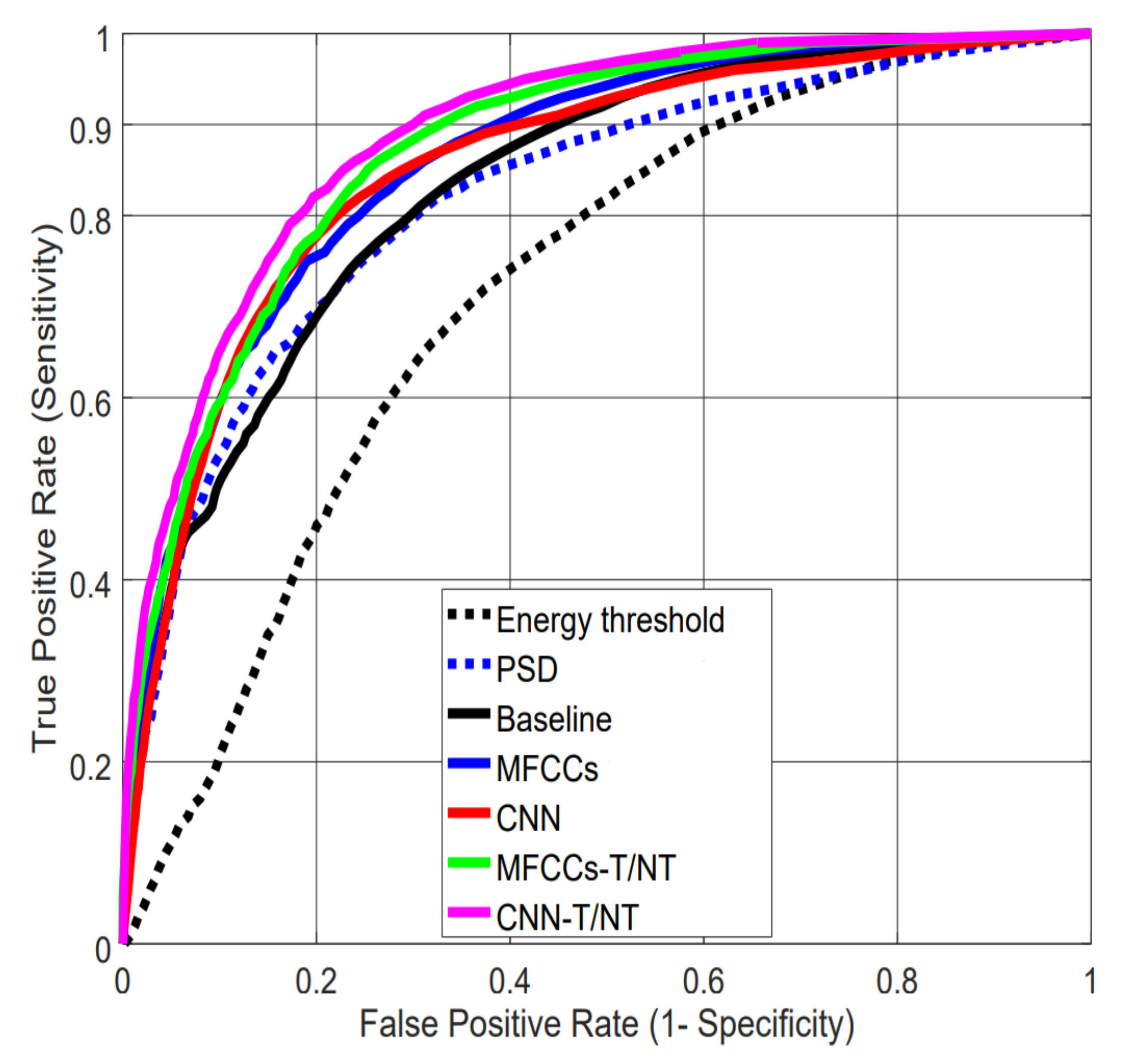
4.1. Evaluating Performance on Lab Data
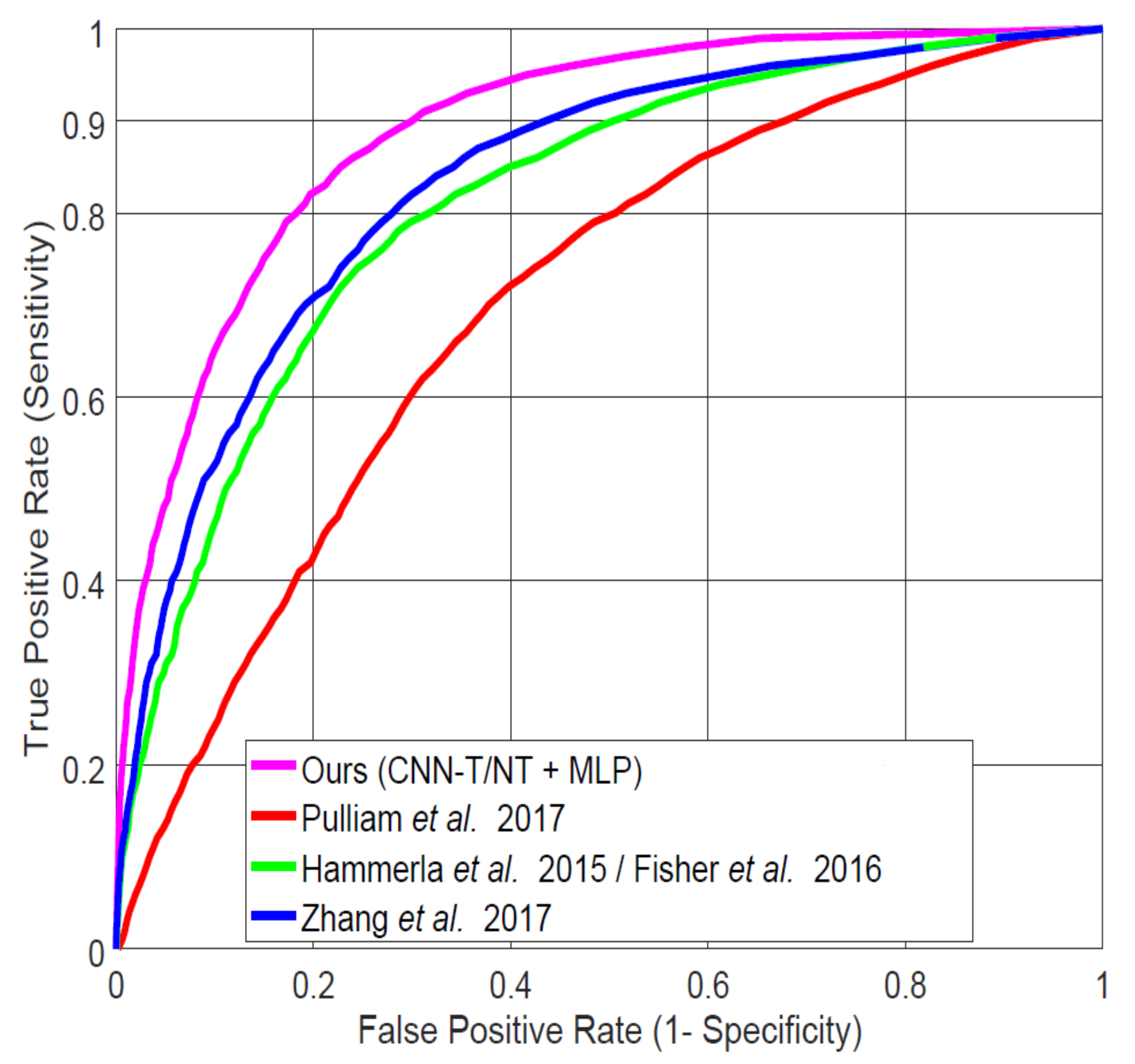
4.2. Comparison to Previous Work on LAB Data
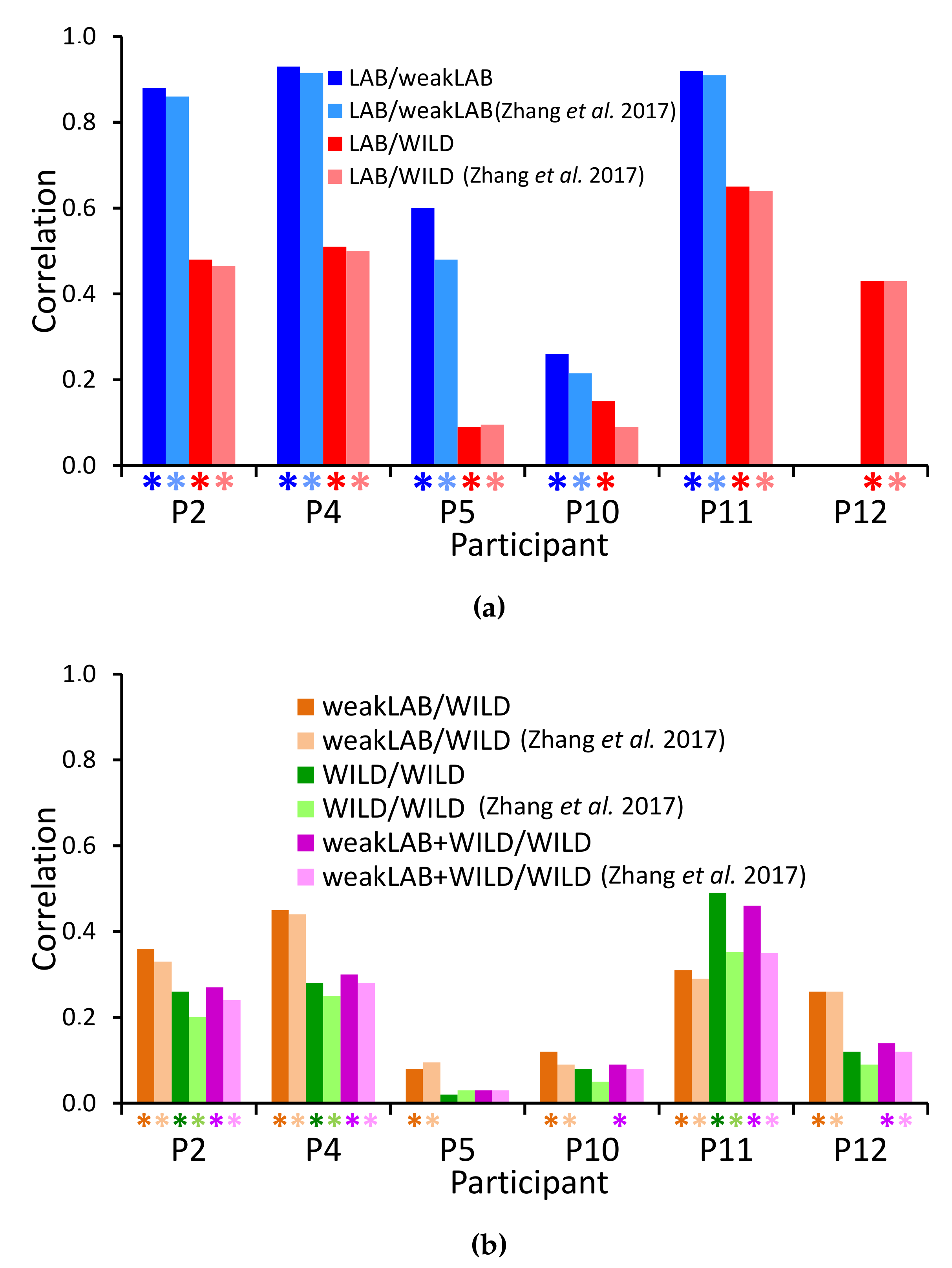
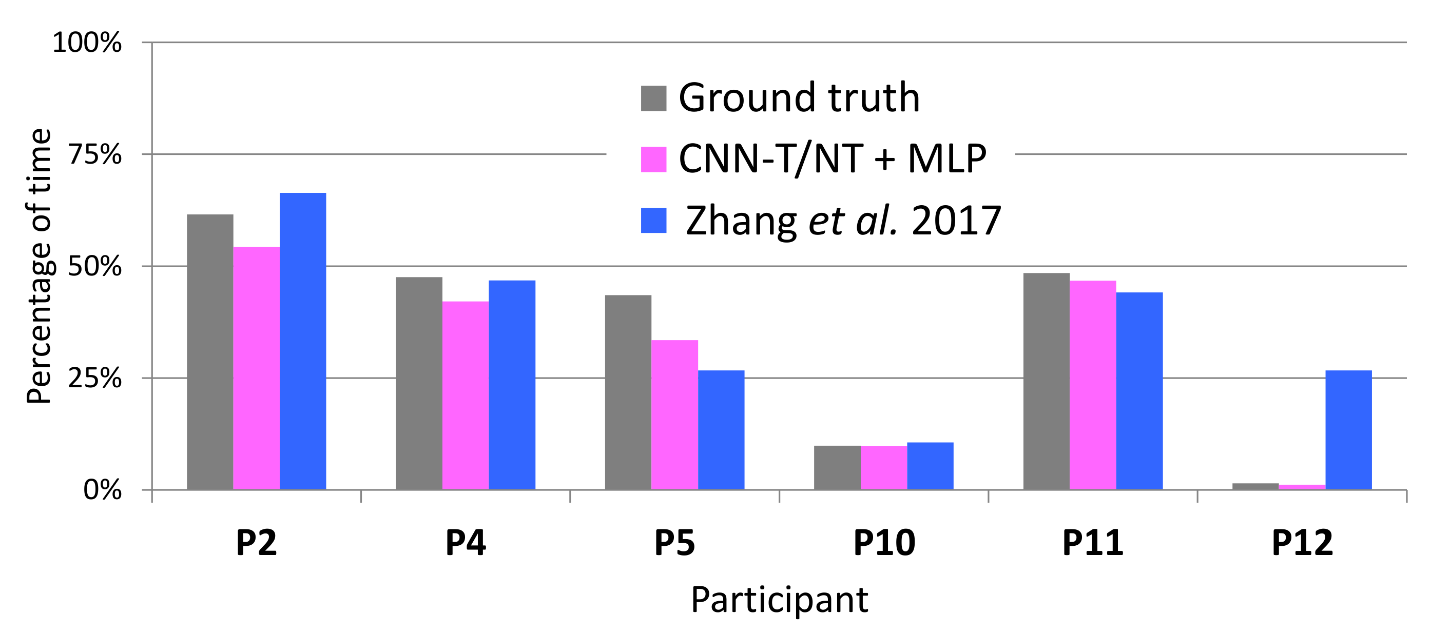
4.3. Reproducing Tremor Self-Assessments in Patients’ Diaries
4.3.1. LAB/WeakLAB
4.3.2. LAB/WILD
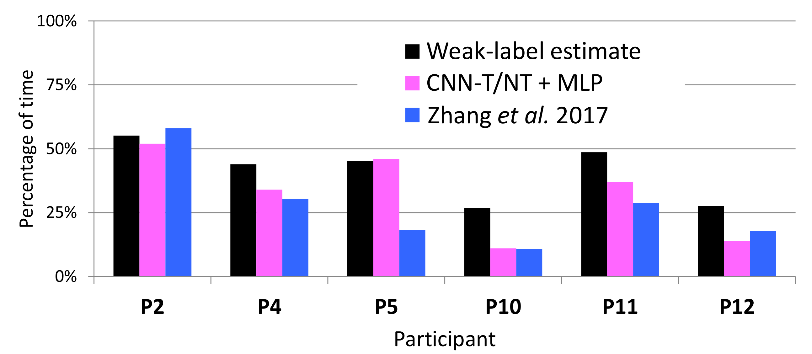
4.3.3. WeakLAB/WILD
4.3.4. WILD/WILD
4.3.5. WeakLAB + WILD/WILD
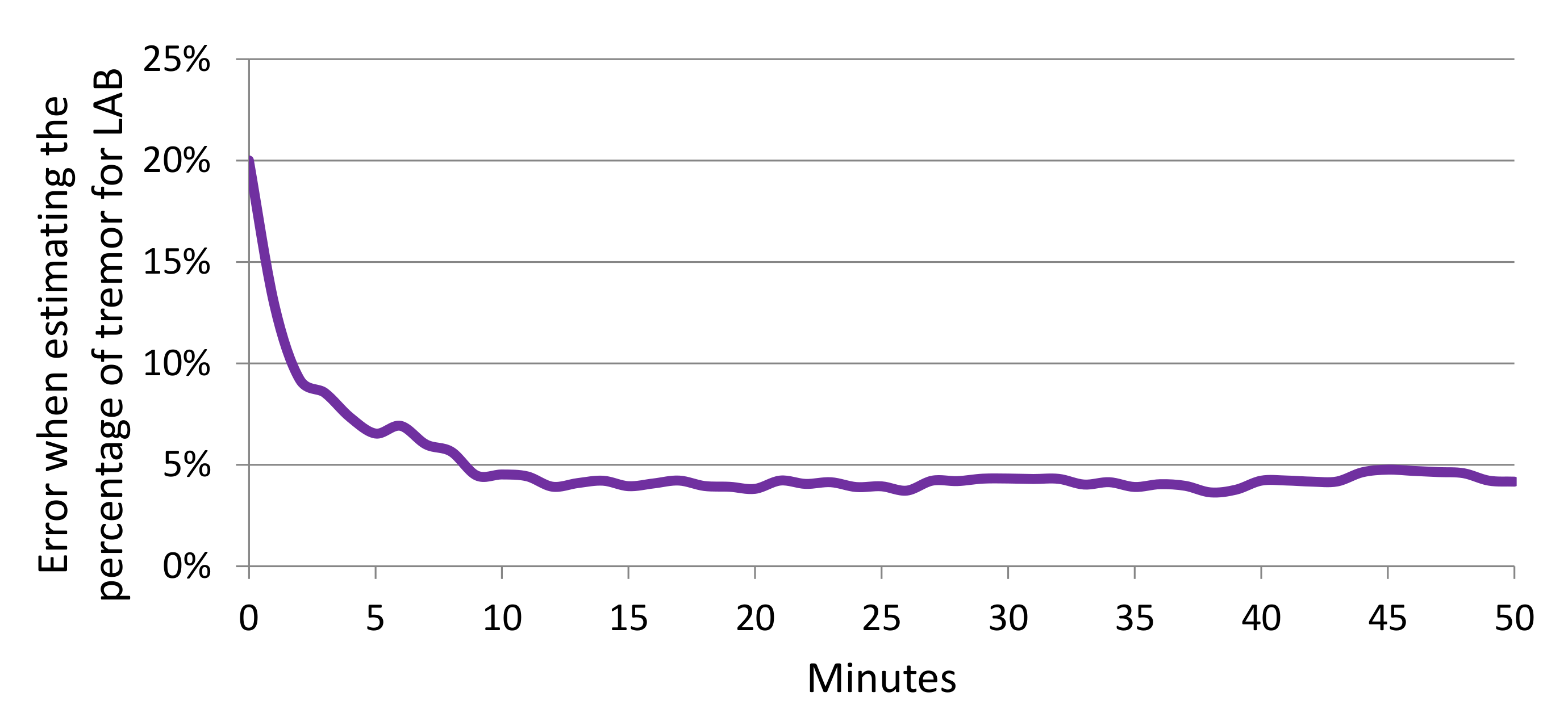
4.4. Estimating Percentage of Tremor Time
5. Conclusions
Author Contributions
Funding
Conflicts of Interest
References
- Shargel, L.; Mutnick, A.H.; Souney, P.F.; Swanson, L.N. Comprehensive Pharmacy Review; L. Williams & Wilkins: Philadelphia, PA, USA, 2008. [Google Scholar]
- Goetz, C.G.; Tilley, B.C.; Shaftman, S.R.; Stebbins, G.T.; Fahn, S.; Martinez-Martin, P.; Poewe, W.; Sampaio, C.; Stern, M.B.; Dodel, R.; et al. Movement Disorder Society-sponsored revision of the Unified Parkinson’s Disease Rating Scale (MDS-UPDRS): Scale presentation and clinimetric testing results. Mov. Disord. 2008, 23, 2129–2170. [Google Scholar] [CrossRef] [PubMed]
- Wiseman, V.; Conteh, L.; Matovu, F. Using diaries to collect data in resource-poor settings: Questions on design and implementation. Health Policy Plan. 2005, 20, 394–404. [Google Scholar] [CrossRef] [PubMed]
- Zhang, A.; Cebulla, A.; Panev, S.; Hodgins, J.; la Torre, F.D. Weakly-supervised learning for Parkinson’s Disease tremor detection. In Proceedings of the 2017 39th Annual International Conference of the IEEE Engineering in Medicine and Biology Society (EMBC), Seogwipo, Korea, 11–15 July 2017; pp. 143–147. [Google Scholar]
- Zhang, A.; De la Torre, F.; Hodgins, J. Comparing laboratory and in-the-wild data for continuous Parkinson’s Disease tremor detection. In Proceedings of the 2020 42nd Annual International Conference of the IEEE Engineering in Medicine and Biology Society (EMBC), Montreal, Canada, 20–24 July 2020; pp. 5436–5441. Available online: https://embc.embs.org/2020/ (accessed on 14 October 2020).
- Pulliam, C.L.; Heldman, D.A.; Brokaw, E.B.; Mera, T.O.; Mari, Z.K.; Burack, M.A. Continuous Assessment of Levodopa Response in Parkinson’s Disease Using Wearable Motion Sensors. IEEE Trans. Biomed. Eng. 2017, 65, 159–164. [Google Scholar] [CrossRef] [PubMed]
- Hammerla, N.Y.; Fisher, J.M.; Andras, P.; Rochester, L.; Walker, R.; Plotz, T. PD Disease State Assessment in Naturalistic Environments Using Deep Learning. In Proceedings of the 2015 29th Conference on Artificial Intelligence (AAAI), Austin, TX, USA, 25–30 January 2015; pp. 1742–1748. [Google Scholar]
- Gockal, E.; Gur, V.E.; Selvitop, R.; Yildiz, G.B.; Asil, T. Motor and Non-Motor Symptoms in Parkinson’s Disease: Effects on Quality of Life. Noro Psikiyatr. Ars. 2017, 54, 143–148. [Google Scholar]
- Iakovakis, D.; Mastoras, R.E.; Hadjidimitriou, S.; Charisis, V.; Bostanjopoulou, S.; Katsarou, Z.; Klingelhoefer, L.; Reichmann, H.; Trivedi, D.; Chaudhuri, R.K.; et al. Smartwatch-based Activity Analysis During Sleep for Early Parkinson’s Disease Detection. In Proceedings of the 2020 42nd Annual International Conference of the IEEE Engineering in Medicine Biology Society (EMBC), Montreal, Canada, 20–24 July 2020; pp. 4326–4329. Available online: https://embc.embs.org/2020/ (accessed on 14 October 2020).
- Kubota, K.J.; Chen, J.A.; Little, M.A. Machine learning for large-scale wearable sensor data in Parkinson’s Disease: Concepts, promises, pitfalls, and futures. Mov. Disord. 2016, 31, 1314–1326. [Google Scholar] [CrossRef]
- Ossig, C.; Antonini, A.; Buhmann, C.; Classen, J.; Csoti, I.; Falkenburger, B.; Schwarz, M.; Winkler, J.; Storch, A. Wearable sensor-based objective assessment of motor symptoms in Parkinson’s disease. J. Neural. Transm. 2016, 123, 57–64. [Google Scholar] [CrossRef]
- Lang, M.; Fietzek, U.; Fröhner, J.; Pfister, F.M.J.; Pichler, D.; Abedinpour, K.; Um, T.T.; Kulic, D.; Endo, S.; Hirche, S. A Multi-layer Gaussian Process for Motor Symptom Estimation in People with Parkinson’s Disease. IEEE Trans. Biomed. Eng. 2019, 3038–3049. [Google Scholar] [CrossRef]
- Cole, B.T.; Roy, S.H.; Luca, C.J.D.; Nawab, S.H. Dynamic neural network detection of tremor and dyskinesia from wearable sensor data. In Proceedings of the 2010 32nd Annual International Conference of the IEEE Engineering in Medicine and Biology Society (EMBC), Buenos Aires, Argentina, 30 August–4 September; pp. 6062–6065.
- García-Magariño, I.; Medrano, C.; Plaza, I.; Oliván, B. A smartphone-based system for detecting hand tremors in unconstrained environments. Pers. Ubiquitous Comput. 2016, 20, 959–971. [Google Scholar] [CrossRef]
- Rigas, G.; Tzallas, A.T.; Tsipouras, M.G.; Bougia, P.; Tripoliti, E.E.; Baga, D.; Fotiadis, D.I.; Tsouli, S.G.; Konitsiotis, S. Assessment of Tremor Activity in the Parkinson’s Disease Using a Set of Wearable Sensors. IEEE Trans. Inf. Technol. Biomed. 2012, 16, 478–487. [Google Scholar] [CrossRef]
- Ahlrichs, C.; Samà Monsonìs, A. Is ’Frequency Distribution’ Enough to Detect Tremor in PD Patients Using a Wrist Worn Accelerometer? In Proceedings of the 2014 8th International Conference on Pervasive Computing Technologies for Healthcare, Oldenburg, Germany, 20–23 May 2014; pp. 65–71. [Google Scholar]
- Patel, S.; Lorincz, K.; Hughes, R.; Huggins, N.; Growdon, J.; Standaert, D.; Akay, M.; Dy, J.; Welsh, M.; Bonato, P. Monitoring Motor Fluctuations in Patients With Parkinson’s Disease Using Wearable Sensors. IEEE Trans. Inf. Technol. Biomed. 2009, 13, 864–873. [Google Scholar] [CrossRef]
- Zwartjes, D.G.M.; Heida, T.; van Vugt, J.P.P.; Geelen, J.A.G.; Veltink, P.H. Ambulatory Monitoring of Activities and Motor Symptoms in Parkinson’s Disease. IEEE Trans. Inf. Technol. Biomed. 2010, 57, 2778–2786. [Google Scholar] [CrossRef]
- Das, S.; Amoedo, B.; De la Torre, F.; Hodgins, J. Detecting Parkinson’s symptoms in uncontrolled home environments: A multiple instance learning approach. In Proceedings of the 2012 34th Conference of the IEEE Engineering in Medicine and Biology Society (EMBC), San Diego, CA, USA, 28 August–1 September 2012; pp. 3688–3691. [Google Scholar]
- Dai, H.; Zhang, P.; Lueth, T.C. Quantitative Assessment of Parkinsonian Tremor Based on an Inertial Measurement Unit. Sensors 2015, 15, 25055–25071. [Google Scholar] [CrossRef] [PubMed]
- San-Segundo, R.; Montero, J.M.; Barra, R.; Fernández, F.; Pardo, J.M. Feature Extraction from Smartphone Inertial Signals for Human Activity Segmentation. Signal Process. 2016, 120, 359–372. [Google Scholar] [CrossRef]
- Vanrell, S.R.; Milone, D.H.; Rufiner, H.L. Assessment of homomorphic analysis for human activity recognition from acceleration signals. IEEE J. Biomed. Health Inform. 2017, 22, 1001–1010. [Google Scholar] [CrossRef] [PubMed]
- Arora, S.; Venkataraman, V.; Zhan, A.; Donohue, S.; Biglan, K.; Dorsey, E.; Little, M. Detecting and monitoring the symptoms of Parkinson’s Disease using smartphones: A pilot study. Parkinsonism Relat. Disord. 2015, 21, 650–653. [Google Scholar] [CrossRef] [PubMed]
- Yao, L.; Brown, P.; Shoaran, M. Resting Tremor Detection in Parkinson’s Disease with Machine Learning and Kalman Filtering. In Proceedings of the 2018 IEEE Biomedical Circuits and Systems Conference (BioCAS), Cleveland, OH, USA, 17–19 October 2018; pp. 1–4. [Google Scholar]
- Stamate, C.; Magoulas, G.D.; Kueppers, S.; Nomikou, E.; Daskalopoulos, I.; Luchini, M.U.; Moussouri, T.; Roussos, G. Deep learning Parkinson’s from smartphone data. In Proceedings of the 2017 IEEE International Conference on Pervasive Computing and Communications (PerCom), Kona, HI, USA, 13–17 March 2017; pp. 31–40. [Google Scholar]
- Eskofier, B.M.; Lee, S.I.; Daneault, J.-F.; Golabchi, F.N.; Ferreira-Carvalho, G.; Vergara-Diaz, G.; Sapienza, S.; Costante, G.; Klucken, J.; Kautz, T.; et al. Recent machine learning advancements in sensor-based mobility analysis: deep learning for Parkinson’s Disease assessment. In Proceedings of the 2016 38th Annual International Conference of the IEEE Engineering in Medicine and Biology Society (EMBC), Orlando, FL, USA, 17–20 August 2016; pp. 655–658. [Google Scholar]
- Um, T.T.; Pfister, F.M.; Pichler, D.; Endo, S.; Lang, M.; Hirche, S.; Fietzek, U.; Kulić, D. Data augmentation of wearable sensor data for Parkinson’s Disease monitoring using convolutional neural networks. In Proceedings of the 19th ACM International Conference on Multimodal Interaction, Glasgow, UK, 13–17 November 2017; pp. 216–220. [Google Scholar]
- Zhan, A.; Little, M.A.; Harris, D.A.; Abiola, S.O.; Dorsey, E.R.; Saria, S.; Terzis, A. High Frequency Remote Monitoring of Parkinson’s Disease via Smartphone: Platform Overview and Medication Response Detection. arXiv 2016, arXiv:1601.00960. [Google Scholar]
- Lipsmeier, F.; Taylor, K.I.; Kilchenmann, T.; Wolf, D.; Scotland, A.; Schjodt-Eriksen, J.; Cheng, W.Y.; Fernandez-Garcia, I.; Siebourg-Polster, J.; Jin, L.; et al. Evaluation of smartphone-based testing to generate exploratory outcome measures in a phase 1 Parkinson’s disease clinical trial. Mov. Disord. 2018, 33, 1287–1297. [Google Scholar] [CrossRef]
- Pulliam, C.; Eichenseer, S.; Goetz, C.; Waln, O.; Hunter, C.; Jankovic, J.; Vaillancourt, D.; Giuffrida, J.; Heldman, D. Continuous in-home monitoring of essential tremor. Park. Relat. Disord. 2014, 20, 37–40. [Google Scholar] [CrossRef] [PubMed]
- Giuffrida, J.P.; Riley, D.E.; Maddux, B.N.; Heldman, D.A. Clinically deployable Kinesia™ technology for automated tremor assessment. Mov. Disord. 2009, 24, 723–730. [Google Scholar] [CrossRef]
- Fisher, J.M.; Hammerla, N.Y.; Ploetz, T.; Andras, P.; Rochester, L.; Walker, R.W. Unsupervised home monitoring of Parkinson’s Disease motor symptoms using body-worn accelerometers. Park. Relat. Disord. 2016, 33, 44–50. [Google Scholar] [CrossRef]
- Heijmans, M.; Habets, J.; Herff, C.; Aarts, J.; Stevens, A.; Kuijf, M.; Kubben, P. Monitoring Parkinson’s disease symptoms during daily life: A feasibility study. NPJ Park. Dis. 2019, 5, 1–6. [Google Scholar] [CrossRef] [PubMed]
- Papadopoulos, A.; Kyritsis, K.; Bostanjopoulou, S.; Klingelhoefer, L.; Chaudhuri, R.K.; Delopoulos, A. Multiple-Instance Learning for In-The-Wild Parkinsonian Tremor Detection. In Proceedings of the 2019 41st Annual International Conference of the IEEE Engineering in Medicine and Biology Society (EMBC), Berlin, Germany, 23–27 July 2019; pp. 6188–6191. [Google Scholar]
- Papadopoulos, A.; Kyritsis, K.; Klingelhoefer, L.; Bostanjopoulou, S.; Chaudhuri, K.R.; Delopoulos, A. Detecting Parkinsonian Tremor From IMU Data Collected in-the-Wild Using Deep Multiple-Instance Learning. IEEE J. Biomed. Health Informatics 2020, 24, 2559–2569. [Google Scholar] [CrossRef] [PubMed]
- Deuschl, G.; Fietzek, U.; Klebe, S.; Volkmann, J. Chapter 24 Clinical neurophysiology and pathophysiology of Parkinsonian tremor. In Handbook of Clinical Neurophysiology; Hallett, M., Ed.; Elsevier: Amsterdam, The Netherlands, 2003; Volume 1, pp. 377–396. [Google Scholar]
- Durrieu, J.L.; David, B.; Richard, G. A Musically Motivated Mid-Level Representation for Pitch Estimation and Musical Audio Source Separation. IEEE J. Sel. Top. Signal Process. 2011, 5, 1180–1191. [Google Scholar] [CrossRef]
- Lee, D.D.; Seung, H.S. Algorithms for Non-negative Matrix Factorization. In Proceedings of the Neural Information Processing Systems 2000 (NIPS 2000), Denver, CO, USA, 27 November–2 December 2000; pp. 556–562. [Google Scholar]
- Hanley, J.A.; McNeil, B.J. The meaning and use of the area under a receiver operating characteristic (ROC) curve. Radiology 1982, 143, 29–36. [Google Scholar] [CrossRef]
- Heldman, D.A.; Jankovic, J.; Vaillancourt, D.E.; Prodoehl, J.; Elble, R.J.; Giuffrida, J.P. Essential Tremor Quantification During Activities of Daily Living. Park. Relat. Disord. 2011, 17, 537–542. [Google Scholar] [CrossRef]
- Siegel, S. Nonparametric Statistics for the Behavioral Sciences; McGraw-Hill: New York, NY, USA, 1956. [Google Scholar]
- Biemans, M.A.J.E.; Dekker, J.; van der Woude, L.H.V. The internal consistency and validity of the Self-assessment Parkinson’s Disease Disability Scale. Clin. Rehabil. 2001, 15, 221–228. [Google Scholar] [CrossRef]
- Martinez-Martin, P.; Rodriguez-Blazquez, C.; Frades-Payo, B. Specific patient-reported outcome measures for Parkinson’s disease: Analysis and applications. Expert Rev. Pharmacoecon. Outcomes Res. 2008, 8, 401–418. [Google Scholar] [CrossRef]
- Luft, F.; Sharifi, S.; Mugge, W.; Schouten, A.C.; Bour, L.J.; Van Rootselaar, A.F.; Veltink, P.H.; Heida, T. Distinct cortical activity patterns in Parkinson’s disease and essential tremor during a bimanual tapping task. J. Neuroeng. Rehabil. 2020, 17, 1–10. [Google Scholar] [CrossRef]
- Heimer, G.; Rivlin-Etzion, M.; Bar-Gad, I.; Goldberg, J.A.; Haber, S.N.; Bergman, H. Dopamine Replacement Therapy Does Not Restore the Full Spectrum of Normal Pallidal Activity in the 1-Methyl-4-Phenyl-1,2,3,6-Tetra-Hydropyridine Primate Model of Parkinsonism. J. Neurosci. 2006, 26, 8101–8114. [Google Scholar] [CrossRef]
- Mahadevan, N.; Demanuele, C.; Zhang, H.; Volfson, D.; Ho, B.; Erb, M.K.; Patel, S. Development of digital biomarkers for resting tremor and bradykinesia using a wrist-worn wearable device. NPJ Digit. Med. 2020, 3, 1–12. [Google Scholar] [CrossRef]


| Participant | Laboratory Session Duration (s) | Left Hand | Right Hand |
|---|---|---|---|
| 2 | 4495 | 80% | 41% |
| 3 | 3351 | 59% | 74% |
| 4 | 3314 | 57% | 37% |
| 5 | 5284 | 39% | 44% |
| 7 | 5824 | 27% | 19% |
| 8 | 5478 | 9% | 38% |
| 9 | 5766 | 22% | 8% |
| 10 | 5070 | 8% | 12% |
| 11 | 3090 | 69% | 26% |
| 12 | 4480 | 2% | 1% |
| Participant # | MDS-UPDRS Task | |||||||||||
|---|---|---|---|---|---|---|---|---|---|---|---|---|
| Resting | Postural | Kinetic | Finger | Hand | Pron. | |||||||
| Tremor | Tremor | Tremor | Tapping | Mov | Sup. | |||||||
| (3.17) | (3.15) | (3.16) | (3.4) | (3.5) | (3.6) | |||||||
| L | R | L | R | L | R | L | R | L | R | L | R | |
| 2 | 2 | 2 | 2 | 1 | 1 | 1 | 1 | 1 | 1 | 0 | 3 | 0 |
| 3 | 1 | 2 | 1 | 2 | 1 | 2 | 1 | 3 | 1 | 2 | 2 | 2 |
| 4 | 3 | 3 | 2 | 3 | 1 | 1 | 3 | 1 | 3 | 1 | 4 | 3 |
| 5 | 0 | 0 | 2 | 2 | 2 | 2 | 2 | 1 | 2 | 1 | 2 | 2 |
| 7 | 0 | 0 | 1 | 1 | 1 | 1 | 1 | 3 | 2 | 3 | 3 | 2 |
| 8 | 1 | 1 | 0 | 1 | 1 | 1 | 1 | 2 | 1 | 2 | 1 | 2 |
| 9 | 0 | 0 | 0 | 0 | 0 | 0 | 3 | 2 | - | 2 | - | 4 |
| 10 | 0 | 2 | 0 | 0 | 1 | 0 | 2 | 3 | 1 | 1 | 2 | 1 |
| 11 | 3 | 0 | 3 | 0 | 1 | 0 | 3 | 1 | 1 | 0 | 1 | 0 |
| 12 | 1 | 1 | 0 | 0 | 0 | 0 | 3 | 2 | 3 | 2 | 2 | 2 |
| Feature Set | AUC | FPR at 0.90 TPR | ||
|---|---|---|---|---|
| RF | MLP | RF | MLP | |
| Energy threshold | 0.715 | 0.62 | ||
| PSD | 0.813 | 0.818 | 0.53 | 0.52 |
| Baseline | 0.830 | 0.829 | 0.45 | 0.45 |
| MFCCs | 0.851 | 0.853 | 0.40 | 0.39 |
| CNN | 0.850 | 0.850 | 0.38 | 0.41 |
| MFCCs-T/NT | 0.869 | 0.870 | 0.33 | 0.33 |
| CNN-T/NT | 0.884 | 0.887 | 0.32 | 0.30 |
| System | AUC | FPR at 0.90 TPR |
|---|---|---|
| CNN-T/NT + MLP (ours) | 0.887 | 0.30 |
| Pulliam et al [30] | 0.701 | 0.67 |
| Hammerla et al. [7]/Fisher et al. [32] | 0.809 | 0.50 |
| Zhang et al. [4] | 0.831 | 0.44 |
| System | LAB Data | WILD Data | ||
|---|---|---|---|---|
| Mean | Std | Mean | Std | |
| CNN-T/NT + MLP (ours) | 4.1% | 4.0% | 9.1% | 5.9% |
| MFCCs-T/NT + MLP (ours) | 4.4% | 5.4% | 12.1% | 8.2% |
| Zhang et al. [4] | 8.8% | 10.0% | 13.7% | 10.1% |
Publisher’s Note: MDPI stays neutral with regard to jurisdictional claims in published maps and institutional affiliations. |
© 2020 by the authors. Licensee MDPI, Basel, Switzerland. This article is an open access article distributed under the terms and conditions of the Creative Commons Attribution (CC BY) license (http://creativecommons.org/licenses/by/4.0/).
Share and Cite
San-Segundo, R.; Zhang, A.; Cebulla, A.; Panev, S.; Tabor, G.; Stebbins, K.; Massa, R.E.; Whitford, A.; de la Torre, F.; Hodgins, J. Parkinson’s Disease Tremor Detection in the Wild Using Wearable Accelerometers. Sensors 2020, 20, 5817. https://doi.org/10.3390/s20205817
San-Segundo R, Zhang A, Cebulla A, Panev S, Tabor G, Stebbins K, Massa RE, Whitford A, de la Torre F, Hodgins J. Parkinson’s Disease Tremor Detection in the Wild Using Wearable Accelerometers. Sensors. 2020; 20(20):5817. https://doi.org/10.3390/s20205817
Chicago/Turabian StyleSan-Segundo, Rubén, Ada Zhang, Alexander Cebulla, Stanislav Panev, Griffin Tabor, Katelyn Stebbins, Robyn E. Massa, Andrew Whitford, Fernando de la Torre, and Jessica Hodgins. 2020. "Parkinson’s Disease Tremor Detection in the Wild Using Wearable Accelerometers" Sensors 20, no. 20: 5817. https://doi.org/10.3390/s20205817
APA StyleSan-Segundo, R., Zhang, A., Cebulla, A., Panev, S., Tabor, G., Stebbins, K., Massa, R. E., Whitford, A., de la Torre, F., & Hodgins, J. (2020). Parkinson’s Disease Tremor Detection in the Wild Using Wearable Accelerometers. Sensors, 20(20), 5817. https://doi.org/10.3390/s20205817