
Mechanical Framework for Geopolymer Gels Construction: An Optimized LSTM Technique to Predict Compressive Strength of Fly Ash-Based Geopolymer Gels Concrete
Abstract
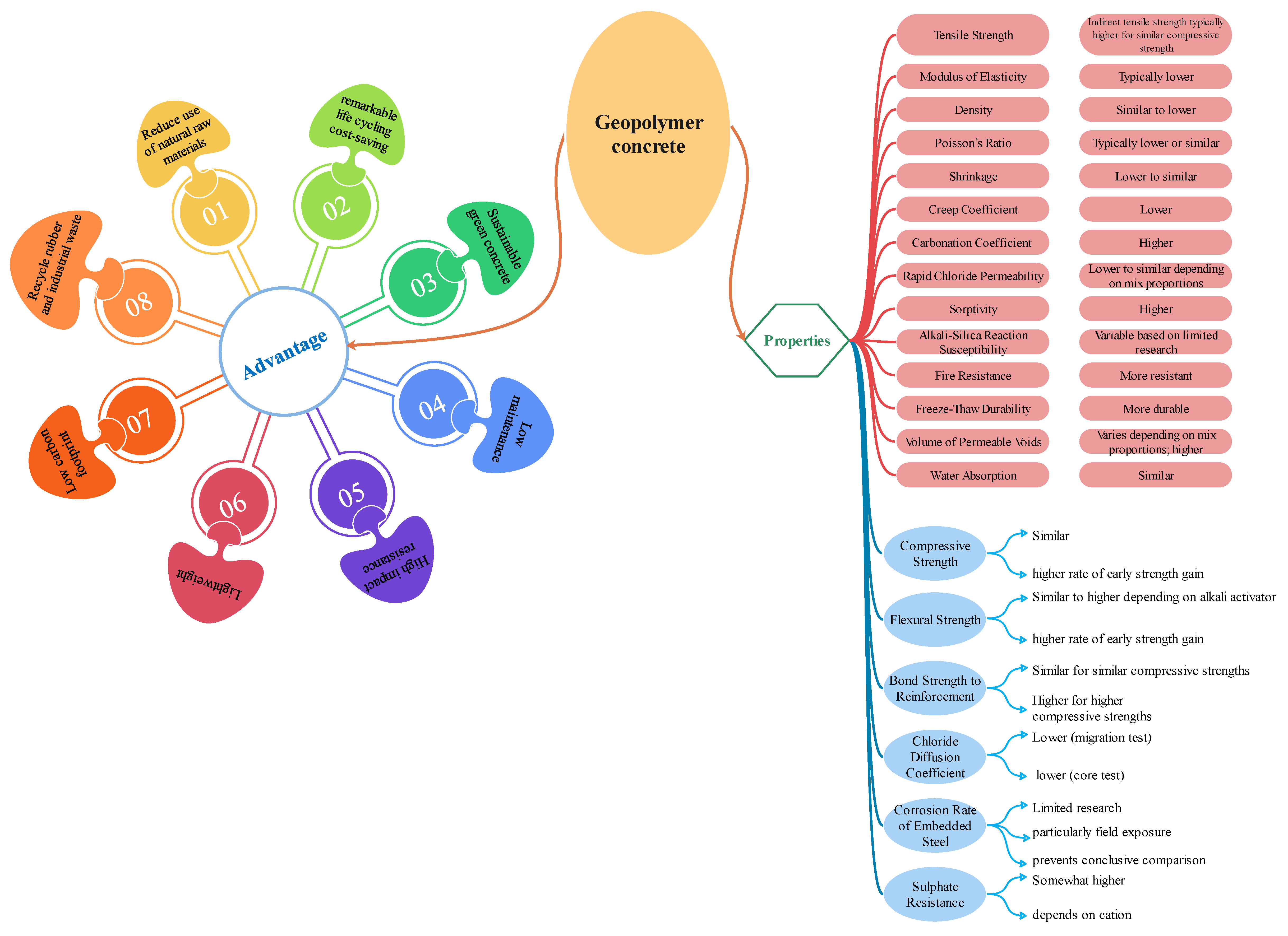
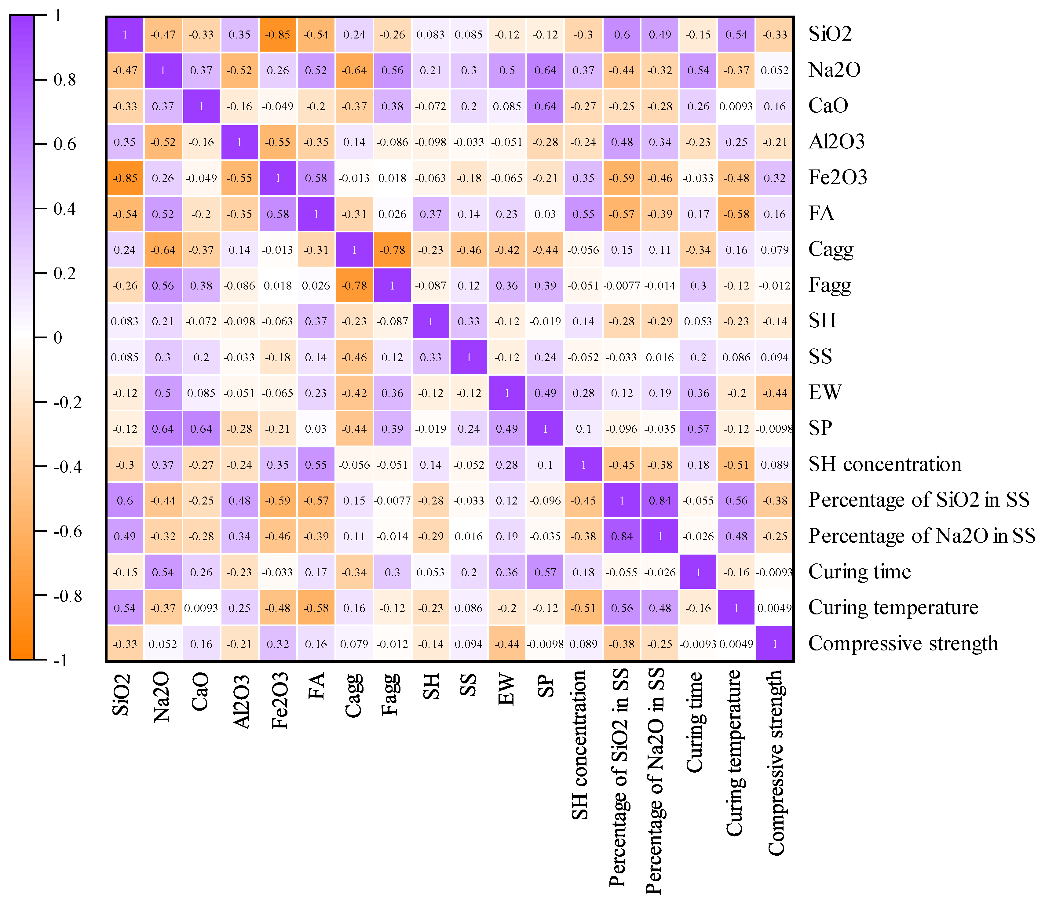
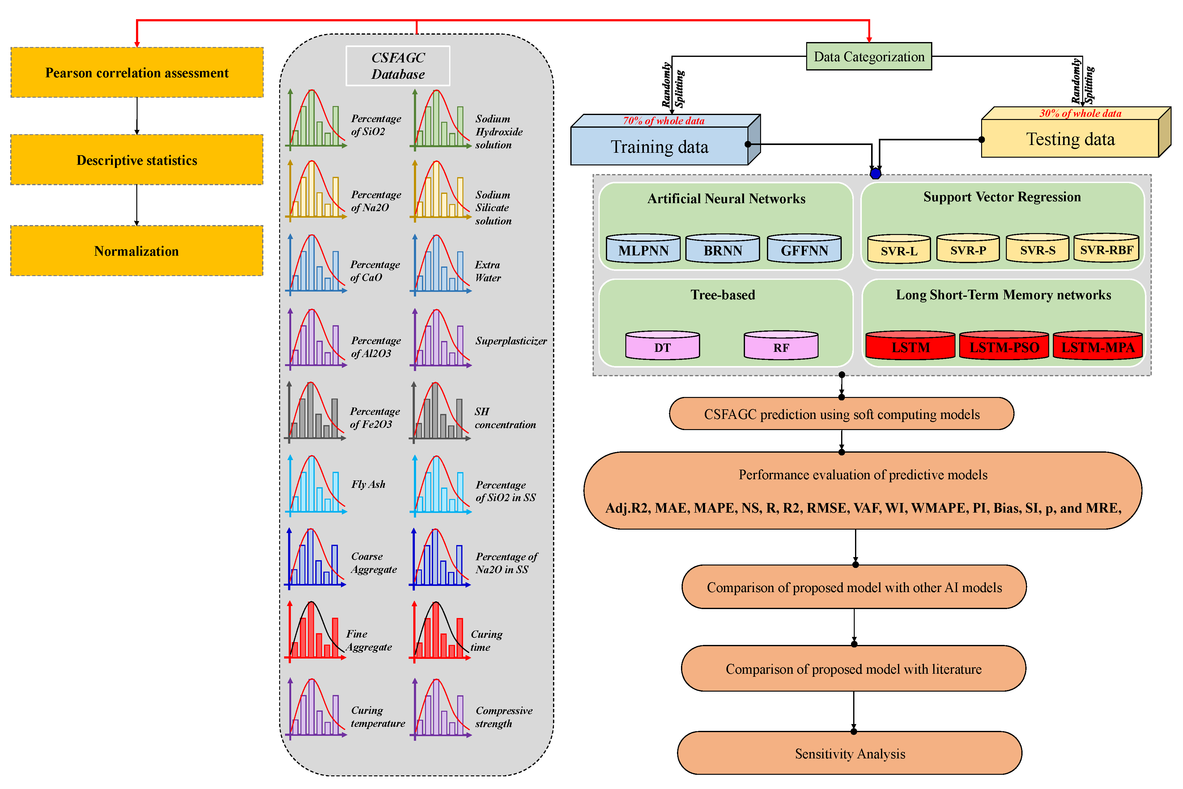
:1. Introduction
2. Results and Discussion
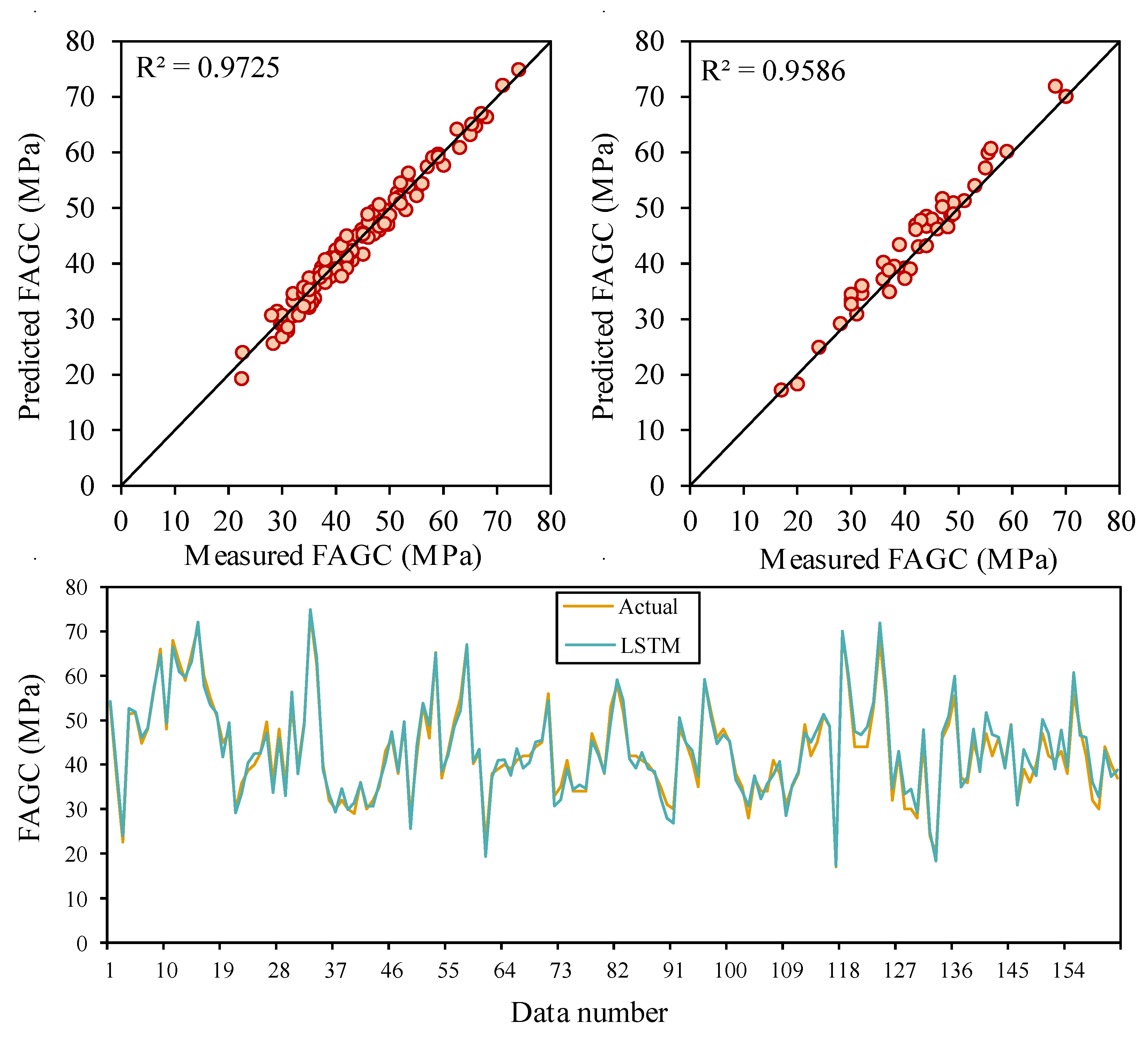
2.1. LSTM
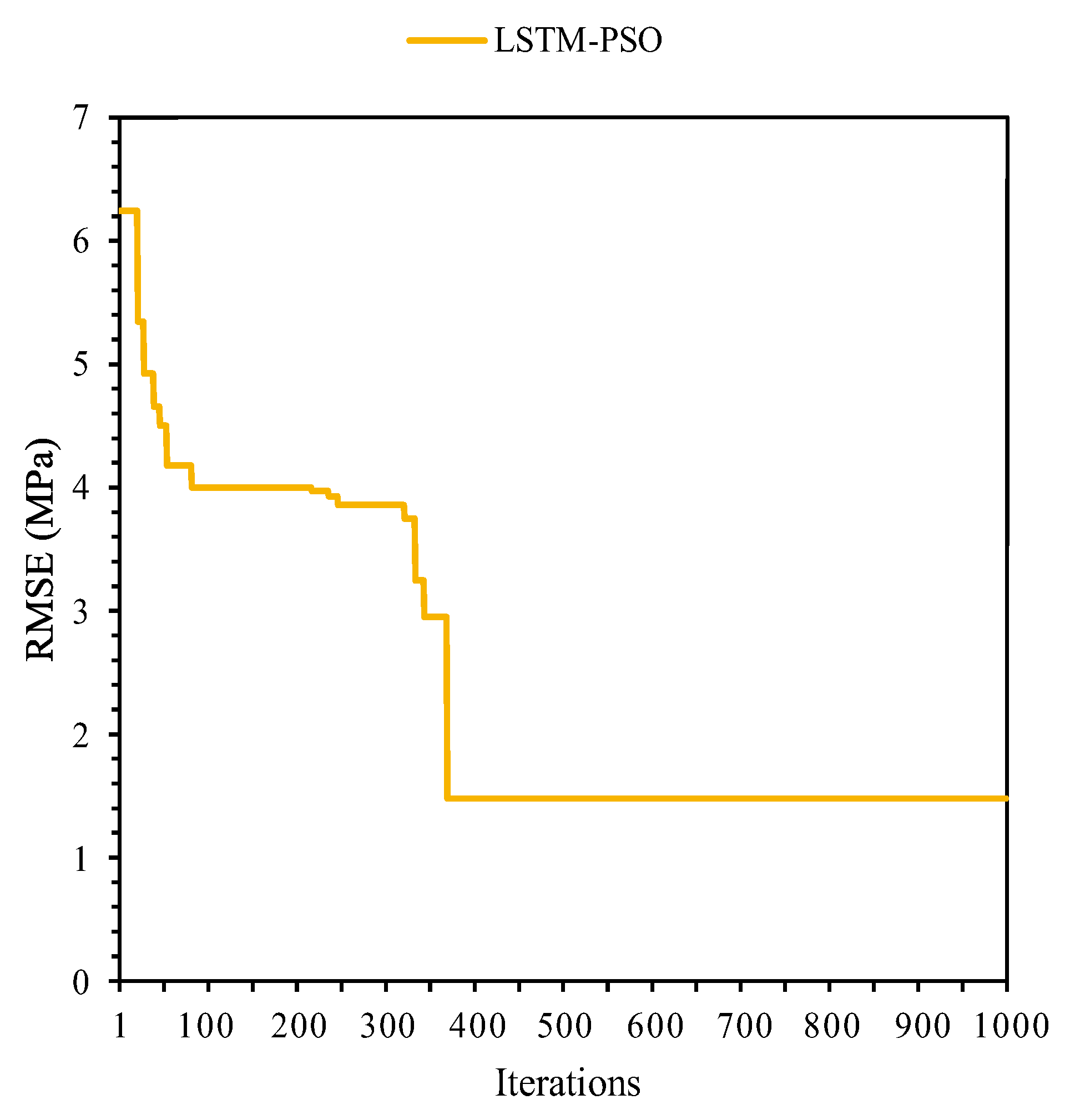
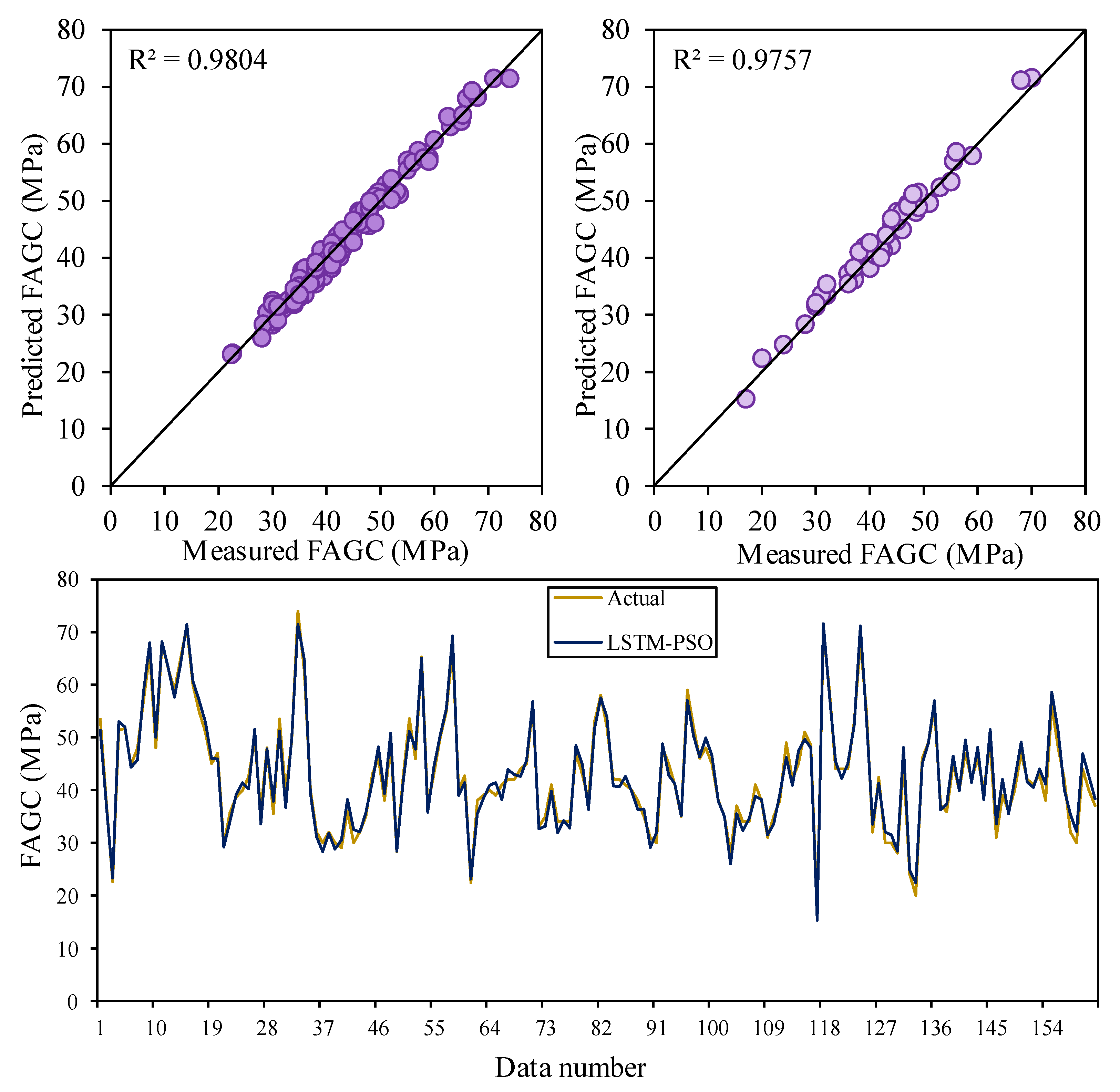
2.2. LSTM-PSO
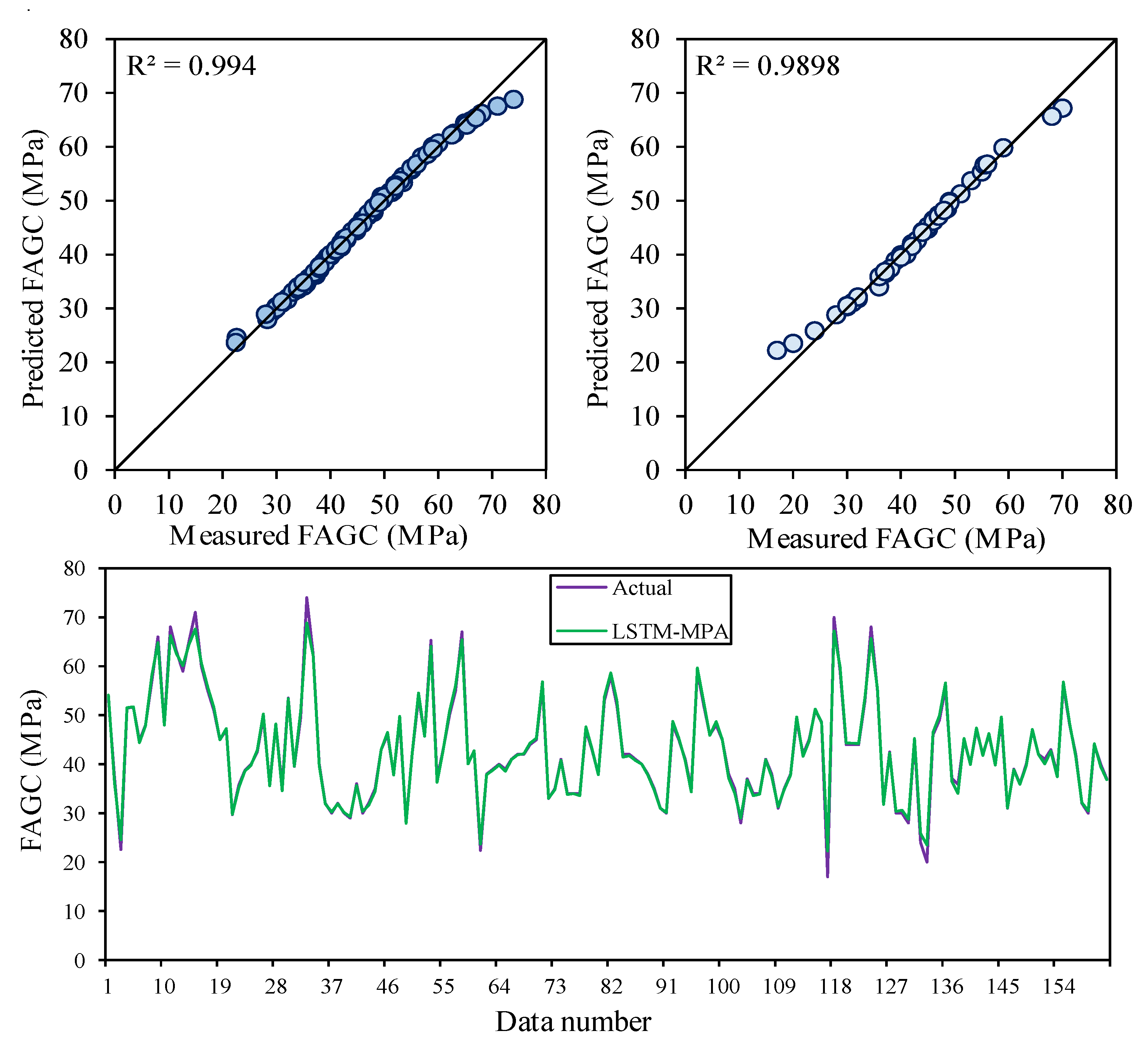
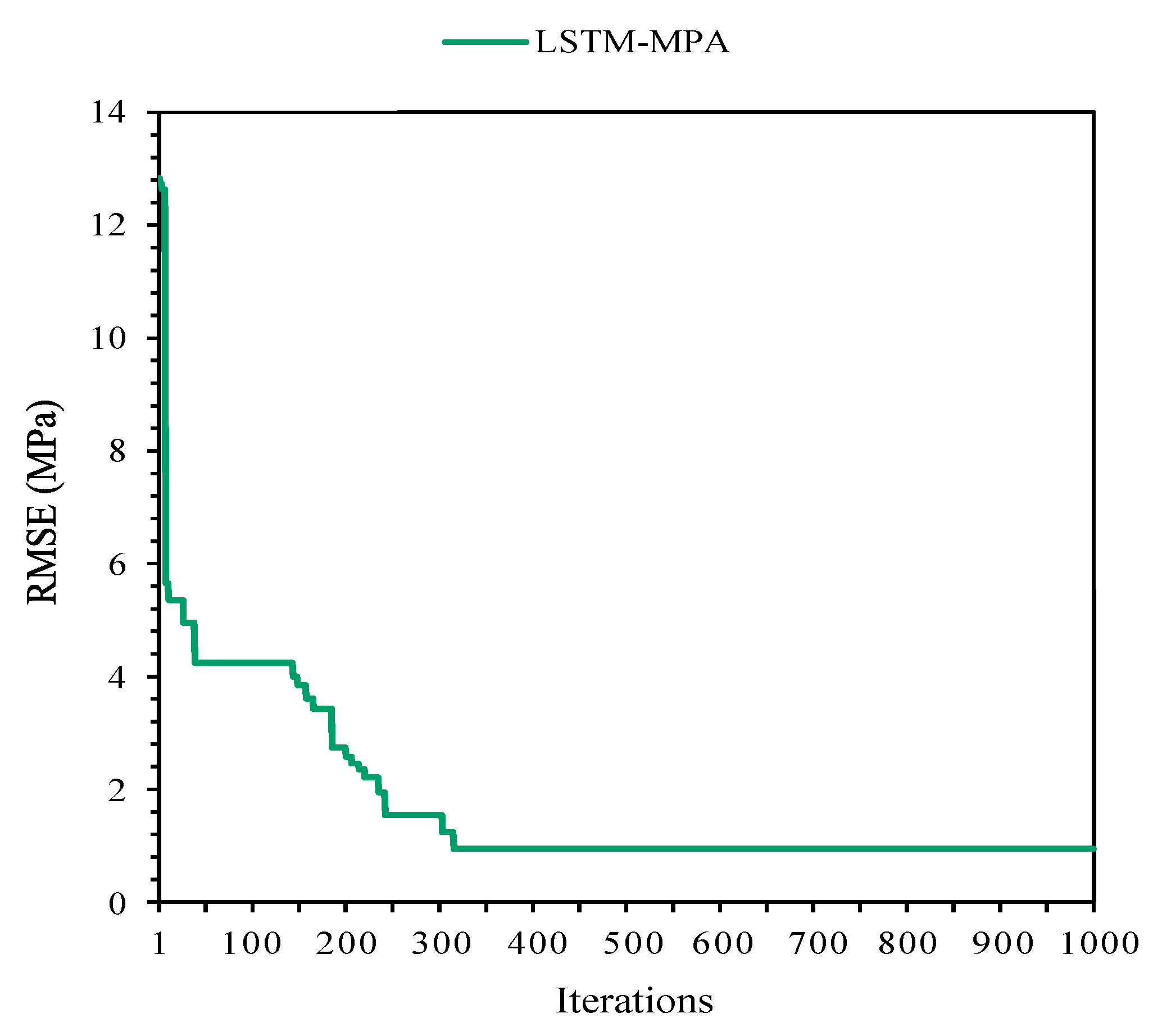
2.3. LSTM-MPA
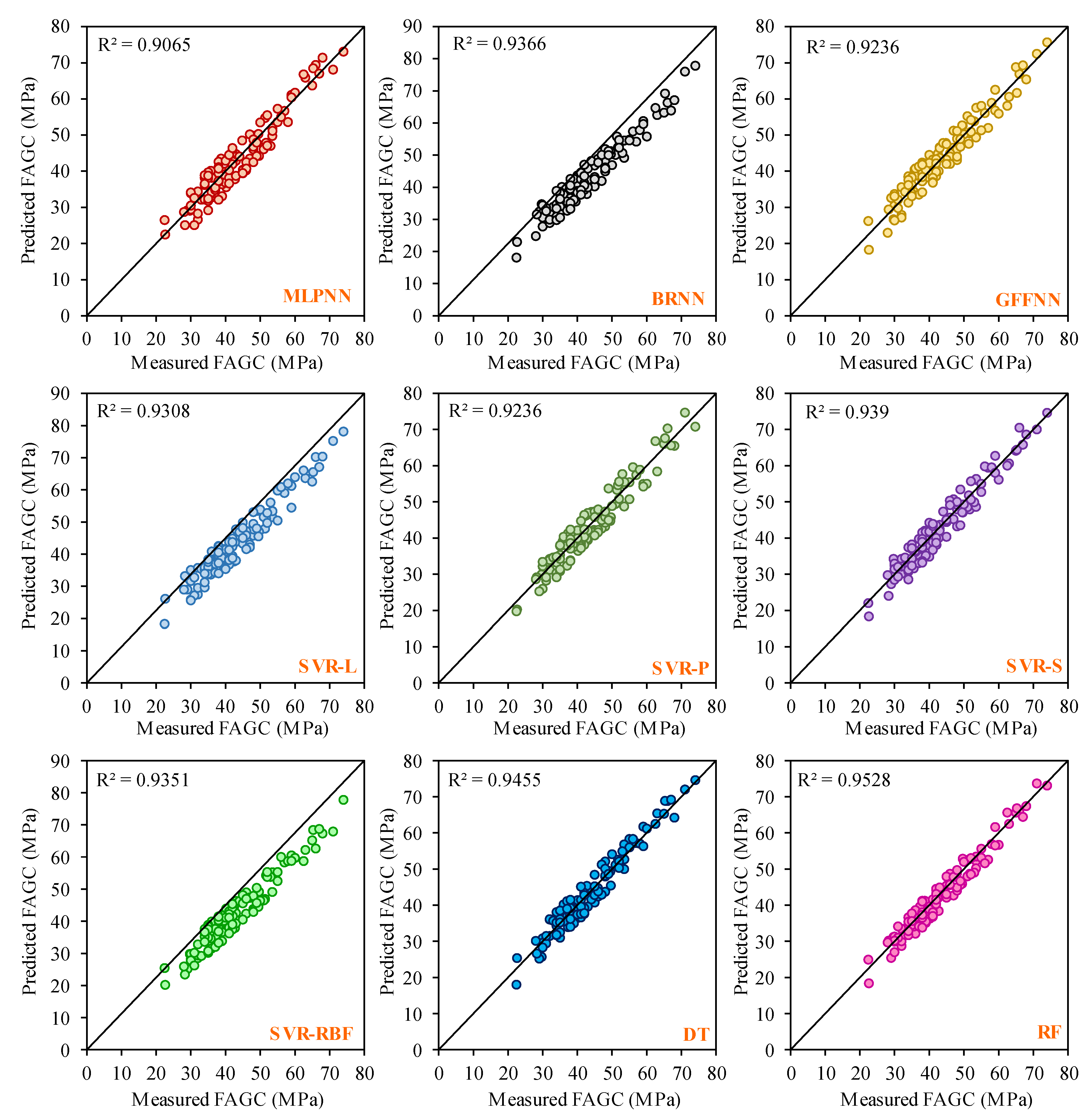
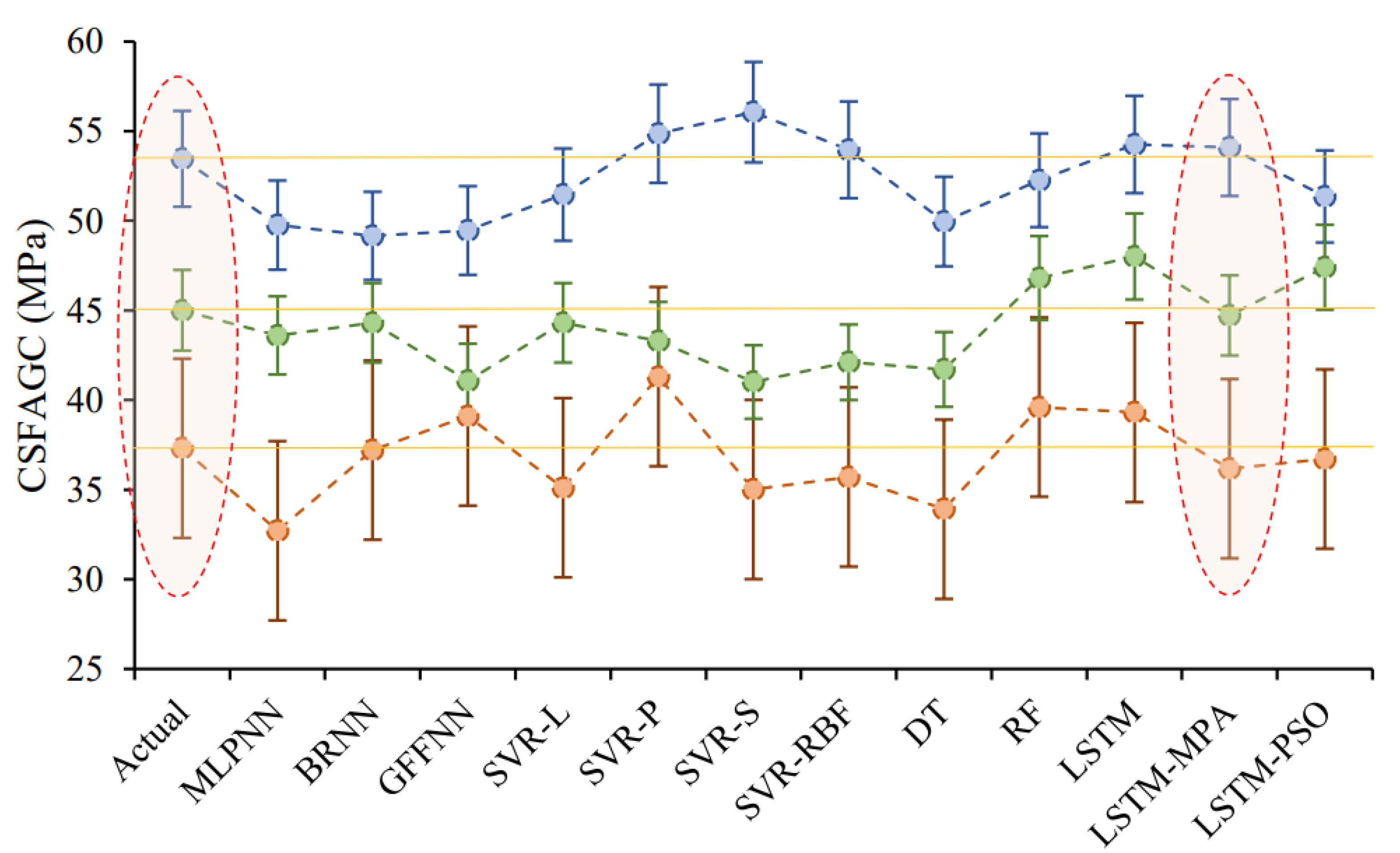
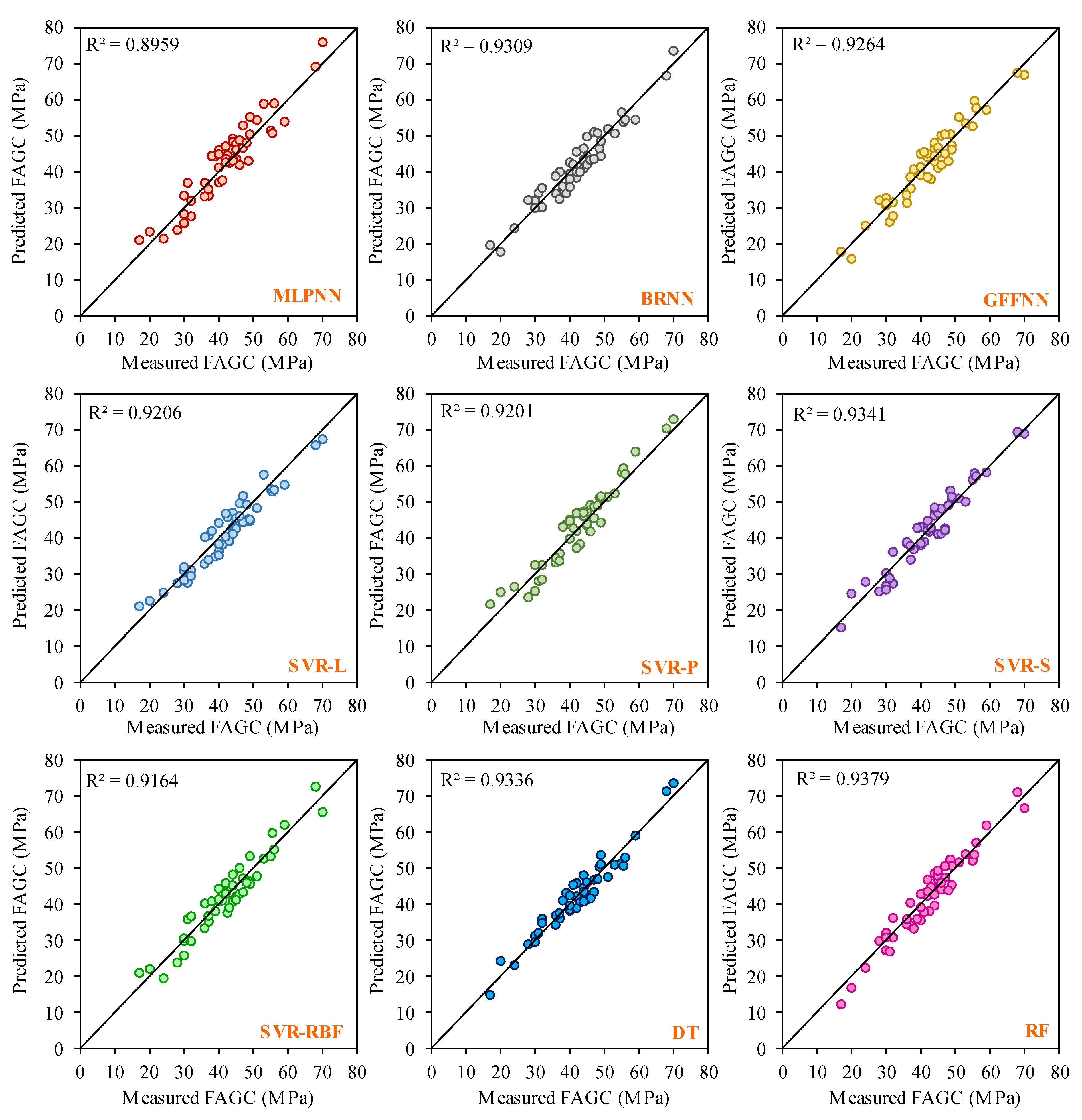
2.4. Comparison of the Proposed Model with Other AI Models
2.5. Comparison of the Proposed Model with the Literature
2.6. Sensitivity Analysis
3. Summary and Conclusions
4. Methods
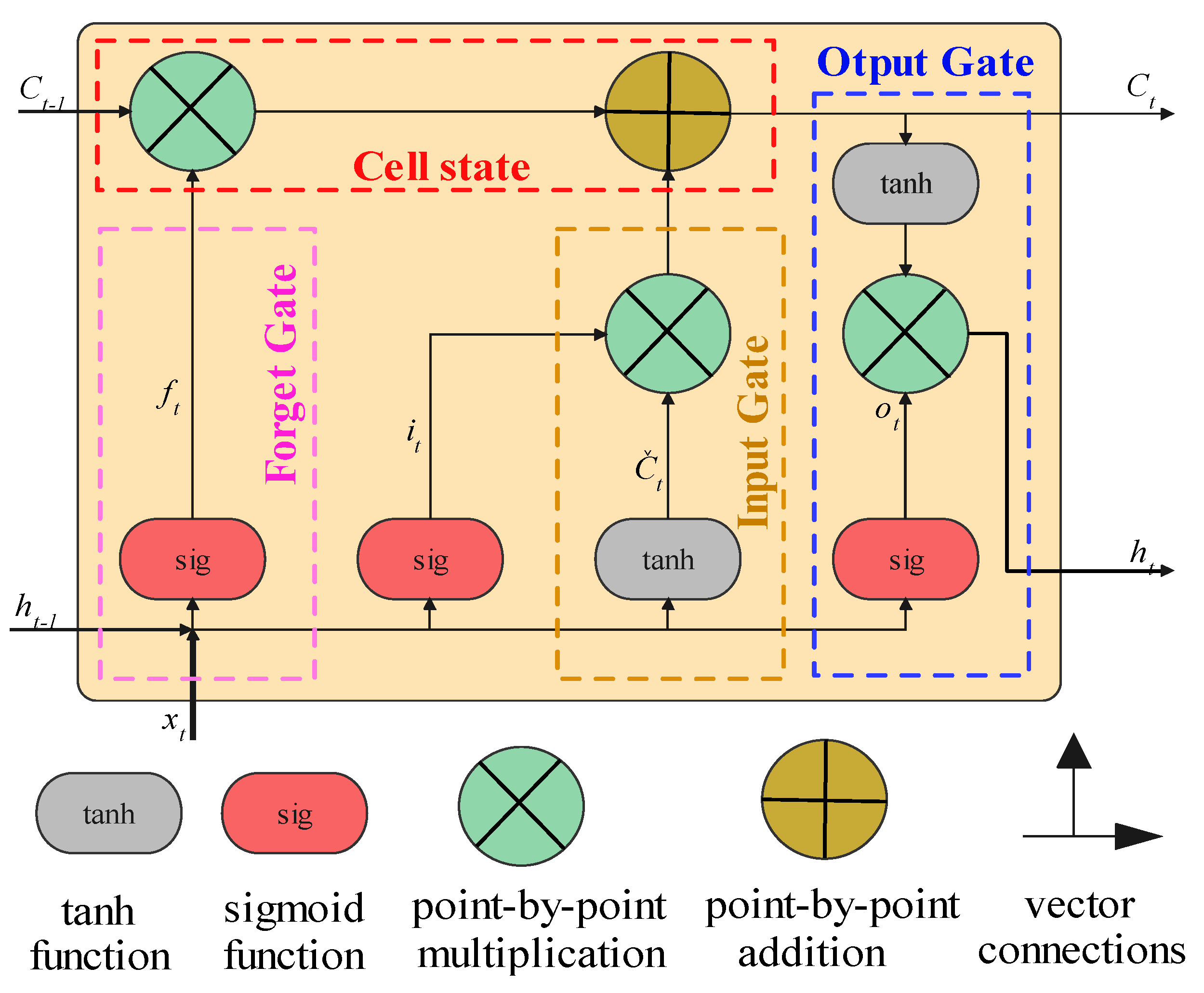
4.1. Long Short-Term Memory Network (LSTM)
4.2. Particle Swarm Optimization (PSO)
4.3. Marine Predators Algorithm (MPA)
- (1)
- Initiate the elite and prey matrices in order to produce the starting individuals. In the following, this algorithm is shown mathematically [129]:
- (2)
- The occurrence of slipping into a local optimum may be successfully avoided by the implementation of the eddy running and the FADs effects, and the mathematical representation of this condition is as follows [129]:where FADs stand for the impact parameter, which is set to 0.18 in our study, K denotes the random binary vector, r indicates a uniform random integer between 0 and 1, and r1 and r2 denote the random hunt in the hunt matrix, respectively.
4.4. Data Description
4.5. Model Validation and Evaluation
4.6. Development of Proposed Model
- (1)
- The MPA is utilized to optimize the hyperparameters (including the number of epochs, number of hidden neurons, batch sizes, dropout rates, and activation functions), as well as to determine their initial values in a general model for the regression of the LSTM.
- (2)
- After training the model with input datasets using the LSTM model from the preceding phase and the hyperparameters’ initial values, Bayesian theory is used to optimize the hyperparameters.
- (3)
- Following the initial metaheuristic algorithm process, the new dataset is imported into the LSTM model to obtain the final estimation result. The initial values of the hyperparameters have been optimized to enable immediate implementation of the optimization problems and prevent the parameter values from quickly falling into an optimal local value.
Author Contributions
Funding
Data Availability Statement
Conflicts of Interest
References
- Masoud, M.A.; El-Khayatt, A.M.; Mahmoud, K.A.; Rashad, A.M.; Shahien, M.G.; Bakhit, B.R.; Zayed, A.M. Valorization of Hazardous Chrysotile by H3BO3 Incorporation to Produce an Innovative Eco-Friendly Radiation Shielding Concrete: Implications on Physico-Mechanical, Hydration, Microstructural, and Shielding Properties. Cem. Concr. Compos. 2023, 141, 105120. [Google Scholar] [CrossRef]
- Masoud, M.A.; Rashad, A.M.; Sakr, K.; Shahien, M.G.; Zayed, A.M. Possibility of Using Different Types of Egyptian Serpentine as Fine and Coarse Aggregates for Concrete Production. Mater. Struct. 2020, 53, 87. [Google Scholar] [CrossRef]
- Masoud, M.A.; El-Khayatt, A.M.; Kansouh, W.A.; Sakr, K.; Shahien, M.G.; Zayed, A.M. Insights into the Effect of the Mineralogical Composition of Serpentine Aggregates on the Radiation Attenuation Properties of Their Concretes. Constr. Build. Mater. 2020, 263, 120141. [Google Scholar] [CrossRef]
- Zayed, A.M.; Masoud, M.A.; Rashad, A.M.; El-Khayatt, A.M.; Sakr, K.; Kansouh, W.A.; Shahien, M.G. Influence of Heavyweight Aggregates on the Physico-Mechanical and Radiation Attenuation Properties of Serpentine-Based Concrete. Constr. Build. Mater. 2020, 260, 120473. [Google Scholar] [CrossRef]
- Zayed, A.M.; Masoud, M.A.; Shahien, M.G.; Gökçe, H.S.; Sakr, K.; Kansouh, W.A.; El-Khayatt, A.M. Physical, Mechanical, and Radiation Attenuation Properties of Serpentine Concrete Containing Boric Acid. Constr. Build. Mater. 2021, 272, 121641. [Google Scholar] [CrossRef]
- Masoud, M.A.; Kansouh, W.A.; Shahien, M.G.; Sakr, K.; Rashad, A.M.; Zayed, A.M. An Experimental Investigation on the Effects of Barite/Hematite on the Radiation Shielding Properties of Serpentine Concretes. Prog. Nucl. Energy 2020, 120, 103220. [Google Scholar] [CrossRef]
- Hendriks, C.A.; Worrell, E.; De Jager, D.; Blok, K.; Riemer, P. Emission Reduction of Greenhouse Gases from the Cement Industry. In Proceedings of the Fourth International Conference on Greenhouse Gas Control Technologies, Interlaken, Switzerland, 30 August–2 September 1998; Volume 30, pp. 939–944. [Google Scholar]
- Hansen, J.; Johnson, D.; Lacis, A.; Lebedeff, S.; Lee, P.; Rind, D.; Russell, G. Climate Impact of Increasing Atmospheric Carbon Dioxide. Science 1981, 213, 957–966. [Google Scholar] [CrossRef]
- Resketi, N.A.; Toufigh, V. Enhancement of Brick-Mortar Shear Bond Strength Using Environmental Friendly Mortars. Constr. Build. Mater. 2019, 195, 28–40. [Google Scholar] [CrossRef]
- Kosarimovahhed, M.; Toufigh, V. Sustainable Usage of Waste Materials as Stabilizer in Rammed Earth Structures. J. Clean. Prod. 2020, 277, 123279. [Google Scholar] [CrossRef]
- McLellan, B.C.; Williams, R.P.; Lay, J.; Van Riessen, A.; Corder, G.D. Costs and Carbon Emissions for Geopolymer Pastes in Comparison to Ordinary Portland Cement. J. Clean. Prod. 2011, 19, 1080–1090. [Google Scholar] [CrossRef]
- Davidovits, J. Geopolymers: Inorganic Polymeric New Materials. J. Therm. Anal. Calorim. 1991, 37, 1633–1656. [Google Scholar] [CrossRef]
- Kong, D.L.Y.; Sanjayan, J.G. Effect of Elevated Temperatures on Geopolymer Paste, Mortar and Concrete. Cem. Concr. Res. 2010, 40, 334–339. [Google Scholar] [CrossRef]
- Hardjito, D.; Rangan, B.V. Development and Properties of Low-Calcium Fly Ash-Based Geopolymer Concrete; Curtin University of Technology: Perth, WA, Australia, 2005. [Google Scholar]
- Liu, J.D.; Li, G.C.; Yang, S.; Huang, J.D. Prediction Models for Evaluating the Strength of Cemented Paste Backfill: A Comparative Study. Minerals 2020, 10, 1041. [Google Scholar] [CrossRef]
- Huang, J.D.; Zhang, Y.; Sun, Y.T.; Ren, J.L.; Zhao, Z.D.; Zhang, J.F. Evaluation of Pore Size Distribution and Permeability Reduction Behavior in Pervious Concrete. Constr. Build. Mater. 2021, 290, 123228. [Google Scholar] [CrossRef]
- Pavithra, P.; Reddy, M.S.; Dinakar, P.; Rao, B.H.; Satpathy, B.K.; Mohanty, A.N. A Mix Design Procedure for Geopolymer Concrete with Fly Ash. J. Clean. Prod. 2016, 133, 117–125. [Google Scholar] [CrossRef]
- Al Bakri, A.M.M.; Kamarudin, H.; Bnhussain, M.; Rafiza, A.; Zarina, Y. Effect of Na2SiO3/NaOH Ratios and NaOH Molarities on Compressive Strength of Fly Ash Based Geopolymer Cement. Green Concr. UniMAP Sch. Mater. Eng. 2010, 1–14. [Google Scholar]
- Phoo-ngernkham, T.; Maegawa, A.; Mishima, N.; Hatanaka, S.; Chindaprasirt, P. Effects of Sodium Hydroxide and Sodium Silicate Solutions on Compressive and Shear Bond Strengths of FA–GBFS Geopolymer. Constr. Build. Mater. 2015, 91, 1–8. [Google Scholar] [CrossRef]
- Joseph, B.; Mathew, G. Influence of Aggregate Content on the Behavior of Fly Ash Based Geopolymer Concrete. Sci. Iran. 2012, 19, 1188–1194. [Google Scholar] [CrossRef]
- Abdulkareem, O.A.; Ramli, M. Optimization of Alkaline Activator Mixing and Curing Conditions for a Fly Ash-Based Geopolymer Paste System. Mod. Appl. Sci. 2015, 9, 61. [Google Scholar] [CrossRef]
- Tang, Z.; Hu, Y.; Tam, V.W.Y.; Li, W. Uniaxial Compressive Behaviors of Fly Ash/Slag-Based Geopolymeric Concrete with Recycled Aggregates. Cem. Concr. Compos. 2019, 104, 103375. [Google Scholar] [CrossRef]
- Ma, C.-K.; Awang, A.Z.; Omar, W. Structural and Material Performance of Geopolymer Concrete: A Review. Constr. Build. Mater. 2018, 186, 90–102. [Google Scholar] [CrossRef]
- Assi, L.N.; Deaver, E.E.; Ziehl, P. Effect of Source and Particle Size Distribution on the Mechanical and Microstructural Properties of Fly Ash-Based Geopolymer Concrete. Constr. Build. Mater. 2018, 167, 372–380. [Google Scholar] [CrossRef]
- De Silva, P.; Sagoe-Crenstil, K.; Sirivivatnanon, V. Kinetics of Geopolymerization: Role of Al2O3 and SiO2. Cem. Concr. Res. 2007, 37, 512–518. [Google Scholar] [CrossRef]
- Davidovits, J.; Davidovits, R. Ferro-Sialate Geopolymers (-Fe-O-Si-O-Al-O-); Geopolymer Institute Library: Saint-Quentin, France, 2020. [Google Scholar]
- Zhou, J.; Su, Z.; Hosseini, S.; Tian, Q.; Lu, Y.; Luo, H.; Xu, X.; Chen, C.; Huang, J. Decision Tree Models for the Estimation of Geo-Polymer Concrete Compressive Strength. Math. Biosci. Eng. 2024, 21, 1413–1444. [Google Scholar] [CrossRef] [PubMed]
- Huang, J.D.; Kumar, G.S.; Sun, Y.T. Evaluation of Workability and Mechanical Properties of Asphalt Binder and Mixture Modified with Waste Toner. Constr. Build. Mater. 2021, 276, 122230. [Google Scholar] [CrossRef]
- Huang, J.D.; Kumar, G.S.; Ren, J.L.; Sun, Y.T.; Li, Y.J.; Wang, C.G. Towards the Potential Usage of Eggshell Powder as Bio-Modifier for Asphalt Binder and Mixture: Workability and Mechanical Properties. Int. J. Pavement Eng. 2022, 23, 3553–3565. [Google Scholar] [CrossRef]
- ASTM C618; A Standard Specification for Coal Fly Ash and Raw or Calcined Natural Pozzolan for Use in Concrete. ASTM International: West Conshohocken, PA, USA, 2019.
- Huang, J.D.; Sun, Y.T.; Zhang, J.F. Reduction of Computational Error by Optimizing SVR Kernel Coefficients to Simulate Concrete Compressive Strength through the Use of a Human Learning Optimization Algorithm. Eng. Comput. 2022, 38, 3151–3168. [Google Scholar] [CrossRef]
- Huang, J.D.; Asteris, P.G.; Pasha, S.M.K.; Mohammed, A.S.; Hasanipanah, M. A New Auto-Tuning Model for Predicting the Rock Fragmentation: A Cat Swarm Optimization Algorithm. Eng. Comput. 2022, 38, 2209–2220. [Google Scholar] [CrossRef]
- Tennakoon, C.; Nazari, A.; Sanjayan, J.G.; Sagoe-Crentsil, K. Distribution of Oxides in Fly Ash Controls Strength Evolution of Geopolymers. Constr. Build. Mater. 2014, 71, 72–82. [Google Scholar] [CrossRef]
- Khedmati, M.; Alanazi, H.; Kim, Y.-R.; Nsengiyumva, G.; Moussavi, S. Effects of Na2O/SiO2 Molar Ratio on Properties of Aggregate-Paste Interphase in Fly Ash-Based Geopolymer Mixtures through Multiscale Measurements. Constr. Build. Mater. 2018, 191, 564–574. [Google Scholar] [CrossRef]
- De Vargas, A.S.; Dal Molin, D.C.C.; Vilela, A.C.F.; Da Silva, F.J.; Pavao, B.; Veit, H. The Effects of Na2O/SiO2 Molar Ratio, Curing Temperature and Age on Compressive Strength, Morphology and Microstructure of Alkali-Activated Fly Ash-Based Geopolymers. Cem. Concr. Compos. 2011, 33, 653–660. [Google Scholar] [CrossRef]
- Ascensão, G.; Marchi, M.; Segata, M.; Faleschini, F.; Pontikes, Y. Reaction Kinetics and Structural Analysis of Alkali Activated Fe–Si–Ca Rich Materials. J. Clean. Prod. 2020, 246, 119065. [Google Scholar] [CrossRef]
- Cui, Y.; Wang, D.; Wang, Y.; Sun, R.; Rui, Y. Effects of the n (H2O: Na2Oeq) Ratio on the Geopolymerization Process and Microstructures of Fly Ash-Based Geopolymers. J. Non-Cryst. Solids 2019, 511, 19–28. [Google Scholar] [CrossRef]
- Song, H.; Ahmad, A.; Farooq, F.; Ostrowski, K.A.; Maślak, M.; Czarnecki, S.; Aslam, F. Predicting the Compressive Strength of Concrete with Fly Ash Admixture Using Machine Learning Algorithms. Constr. Build. Mater. 2021, 308, 125021. [Google Scholar] [CrossRef]
- Farooq, F.; Czarnecki, S.; Niewiadomski, P.; Aslam, F.; Alabduljabbar, H.; Ostrowski, K.A.; Śliwa-Wieczorek, K.; Nowobilski, T.; Malazdrewicz, S. A Comparative Study for the Prediction of the Compressive Strength of Self-Compacting Concrete Modified with Fly Ash. Materials 2021, 14, 4934. [Google Scholar] [CrossRef]
- Khan, M.A.; Memon, S.A.; Farooq, F.; Javed, M.F.; Aslam, F.; Alyousef, R. Compressive Strength of Fly-Ash-Based Geopolymer Concrete by Gene Expression Programming and Random Forest. Adv. Civ. Eng. 2021, 2021, 6618407. [Google Scholar] [CrossRef]
- Ilyas, I.; Zafar, A.; Javed, M.F.; Farooq, F.; Aslam, F.; Musarat, M.A.; Vatin, N.I. Forecasting Strength of CFRP Confined Concrete Using Multi Expression Programming. Materials 2021, 14, 7134. [Google Scholar] [CrossRef] [PubMed]
- Farooq, F.; Nasir Amin, M.; Khan, K.; Rehan Sadiq, M.; Javed, M.F.; Aslam, F.; Alyousef, R. A Comparative Study of Random Forest and Genetic Engineering Programming for the Prediction of Compressive Strength of High Strength Concrete (HSC). Appl. Sci. 2020, 10, 7330. [Google Scholar] [CrossRef]
- Raza, F.; Alshameri, B.; Jamil, S.M. Assessment of Triple Bottom Line of Sustainability for Geotechnical Projects. Environ. Dev. Sustain. 2021, 23, 4521–4558. [Google Scholar] [CrossRef]
- Javed, M.F.; Farooq, F.; Memon, S.A.; Akbar, A.; Khan, M.A.; Aslam, F.; Alyousef, R.; Alabduljabbar, H.; Rehman, S.K.U. New Prediction Model for the Ultimate Axial Capacity of Concrete-Filled Steel Tubes: An Evolutionary Approach. Crystals 2020, 10, 741. [Google Scholar] [CrossRef]
- Nafees, A.; Javed, M.F.; Khan, S.; Nazir, K.; Farooq, F.; Aslam, F.; Musarat, M.A.; Vatin, N.I. Predictive Modeling of Mechanical Properties of Silica Fume-Based Green Concrete Using Artificial Intelligence Approaches: MLPNN, ANFIS, and GEP. Materials 2021, 14, 7531. [Google Scholar] [CrossRef]
- Asteris, P.G.; Lourenço, P.B.; Roussis, P.C.; Adami, C.E.; Armaghani, D.J.; Cavaleri, L.; Chalioris, C.E.; Hajihassani, M.; Lemonis, M.E.; Mohammed, A.S. Revealing the Nature of Metakaolin-Based Concrete Materials Using Artificial Intelligence Techniques. Constr. Build. Mater. 2022, 322, 126500. [Google Scholar] [CrossRef]
- Barkhordari, M.S.; Armaghani, D.J.; Mohammed, A.S.; Ulrikh, D.V. Data-Driven Compressive Strength Prediction of Fly Ash Concrete Using Ensemble Learner Algorithms. Buildings 2022, 12, 132. [Google Scholar] [CrossRef]
- Liao, J.; Asteris, P.G.; Cavaleri, L.; Mohammed, A.S.; Lemonis, M.E.; Tsoukalas, M.Z.; Skentou, A.D.; Maraveas, C.; Koopialipoor, M.; Armaghani, D.J. Novel Fuzzy-Based Optimization Approaches for the Prediction of Ultimate Axial Load of Circular Concrete-Filled Steel Tubes. Buildings 2021, 11, 629. [Google Scholar] [CrossRef]
- Biswas, R.; Bardhan, A.; Samui, P.; Rai, B.; Nayak, S.; Armaghani, D.J. Efficient Soft Computing Techniques for the Prediction of Compressive Strength of Geopolymer Concrete. Comput. Concr. 2021, 28, 221. [Google Scholar] [CrossRef]
- Apostolopoulou, M.; Asteris, P.G.; Armaghani, D.J.; Douvika, M.G.; Lourenço, P.B.; Cavaleri, L.; Bakolas, A.; Moropoulou, A. Mapping and Holistic Design of Natural Hydraulic Lime Mortars. Cem. Concr. Res. 2020, 136, 106167. [Google Scholar] [CrossRef]
- Koopialipoor, M.; Asteris, P.G.; Salih Mohammed, A.; Alexakis, D.E.; Mamou, A.; Armaghani, D.J. Introducing Stacking Machine Learning Approaches for the Prediction of Rock Deformation. Transp. Geotech. 2022, 34, 100756. [Google Scholar] [CrossRef]
- Armaghani, D.J.; Asteris, P.G. A Comparative Study of ANN and ANFIS Models for the Prediction of Cement-Based Mortar Materials Compressive Strength. Neural Comput. Appl. 2021, 33, 4501–4532. [Google Scholar] [CrossRef]
- Iqbal, M.F.; Liu, Q.F.; Azim, I.; Zhu, X.; Yang, J.; Javed, M.F.; Rauf, M. Prediction of Mechanical Properties of Green Concrete Incorporating Waste Foundry Sand Based on Gene Expression Programming. J. Hazard. Mater. 2020, 384, 121322. [Google Scholar] [CrossRef] [PubMed]
- Golafshani, E.M.; Behnood, A. Predicting the Mechanical Properties of Sustainable Concrete Containing Waste Foundry Sand Using Multi-Objective ANN Approach. Constr. Build. Mater. 2021, 291, 123314. [Google Scholar] [CrossRef]
- Sun, Y.; Hanhan, I.; Sangid, M.D.; Lin, G. Predicting Mechanical Properties from Microstructure Images in Fiber-Reinforced Polymers Using Convolutional Neural Networks. arXiv preprint, 2020; arXiv:2010.03675. [Google Scholar]
- Kabiru, O.A.; Owolabi, T.O.; Ssennoga, T.; Olatunji, S.O. Performance Comparison of SVM and ANN in Predicting Compressive Strength of Concrete. J. Comput. Eng. 2014, 16, 88–94. [Google Scholar]
- Belalia Douma, O.; Boukhatem, B.; Ghrici, M.; Tagnit-Hamou, A. Prediction of Properties of Self-Compacting Concrete Containing Fly Ash Using Artificial Neural Network. Neural Comput. Appl. 2017, 28, 707–718. [Google Scholar] [CrossRef]
- Abu Yaman, M.; Abd Elaty, M.; Taman, M. Predicting the Ingredients of Self Compacting Concrete Using Artificial Neural Network. Alex. Eng. J. 2017, 56, 523–532. [Google Scholar] [CrossRef]
- Kaveh, A.; Bakhshpoori, T.; Hamze-Ziabari, S.M. M5’ and Mars Based Prediction Models for Properties of Selfcompacting Concrete Containing Fly Ash. Period. Polytech. Civ. Eng. 2018, 62, 281–294. [Google Scholar] [CrossRef]
- Sathyan, D.; Anand, K.B.; Prakash, A.J.; Premjith, B. Modeling the Fresh and Hardened Stage Properties of Self-Compacting Concrete Using Random Kitchen Sink Algorithm. Int. J. Concr. Struct. Mater. 2018, 12, 24. [Google Scholar] [CrossRef]
- Vakhshouri, B.; Nejadi, S. Prediction of Compressive Strength of Self-Compacting Concrete by ANFIS Models. Neurocomputing 2018, 280, 13–22. [Google Scholar] [CrossRef]
- Naderpour, H.; Rafiean, A.H.; Fakharian, P. Compressive Strength Prediction of Environmentally Friendly Concrete Using Artificial Neural Networks. J. Build. Eng. 2018, 16, 213–219. [Google Scholar] [CrossRef]
- Sarir, P.; Chen, J.; Asteris, P.G.; Armaghani, D.J.; Tahir, M.M. Developing GEP Tree-Based, Neuro-Swarm, and Whale Optimization Models for Evaluation of Bearing Capacity of Concrete-Filled Steel Tube Columns. Eng. Comput. 2021, 37, 1–19. [Google Scholar] [CrossRef]
- Huang, J.; Zhou, M.; Zhang, J.; Ren, J.; Vatin, N.I.; Sabri, M.M.S. Development of a new stacking model to evaluate the strength parameters of concrete samples in laboratory. Iran. J. Sci. Technol. Trans. Civ. Eng. 2022, 46, 4355–4370. [Google Scholar] [CrossRef]
- Asteris, P.G.; Kolovos, K.G. Self-Compacting Concrete Strength Prediction Using Surrogate Models. Neural Comput. Appl. 2019, 31, 409–424. [Google Scholar] [CrossRef]
- Selvaraj, S.; Sivaraman, S. Prediction Model for Optimized Self-Compacting Concrete with Fly Ash Using Response Surface Method Based on Fuzzy Classification. Neural Comput. Appl. 2019, 31, 1365–1373. [Google Scholar] [CrossRef]
- Zhang, J.; Ma, G.; Huang, Y.; Sun, J.; Aslani, F.; Nener, B. Modelling Uniaxial Compressive Strength of Lightweight Self-Compacting Concrete Using Random Forest Regression. Constr. Build. Mater. 2019, 210, 713–719. [Google Scholar] [CrossRef]
- Prachasaree, W.; Limkatanyu, S.; Hawa, A.; Sukontasukkul, P.; Chindaprasirt, P. Manuscript Title: Development of Strength Prediction Models for Fly Ash Based Geopolymer Concrete. J. Build. Eng. 2020, 32, 101704. [Google Scholar] [CrossRef]
- Azimi-Pour, M.; Eskandari-Naddaf, H.; Pakzad, A. Linear and Non-Linear SVM Prediction for Fresh Properties and Compressive Strength of High Volume Fly Ash Self-Compacting Concrete. Constr. Build. Mater. 2020, 230, 117021. [Google Scholar] [CrossRef]
- Saha, P.; Debnath, P.; Thomas, P. Prediction of Fresh and Hardened Properties of Self-Compacting Concrete Using Support Vector Regression Approach. Neural Comput. Appl. 2020, 32, 7995–8010. [Google Scholar] [CrossRef]
- Shahmansouri, A.A.; Akbarzadeh Bengar, H.; Jahani, E. Predicting Compressive Strength and Electrical Resistivity of Eco-Friendly Concrete Containing Natural Zeolite via GEP Algorithm. Constr. Build. Mater. 2019, 229, 116883. [Google Scholar] [CrossRef]
- Aslam, F.; Farooq, F.; Amin, M.N.; Khan, K.; Waheed, A.; Akbar, A.; Javed, M.F.; Alyousef, R.; Alabdulijabbar, H. Applications of Gene Expression Programming for Estimating Compressive Strength of High-Strength Concrete. Adv. Civ. Eng. 2020, 2020, 8850535. [Google Scholar] [CrossRef]
- Shahmansouri, A.A.; Akbarzadeh Bengar, H.; Ghanbari, S. Compressive Strength Prediction of Eco-Efficient GGBS-Based Geopolymer Concrete Using GEP Method. J. Build. Eng. 2020, 31, 101326. [Google Scholar] [CrossRef]
- Buši, R. Prediction Models for the Mechanical Properties of Self-Compacting Concrete with Recycled Rubber and Silica Fume. Materials 2020, 13, 1821. [Google Scholar] [CrossRef]
- Al-mughanam, T.; Aldhyani, T.H.H.; Alsubari, B.; Al-yaari, M. Modeling of Compressive Strength of Sustainable Self-Compacting Concrete Incorporating Treated Palm Oil Fuel Ash Using Artificial Neural Network. Sustainability 2020, 12, 9322. [Google Scholar] [CrossRef]
- Nematzadeh, M.; Shahmansouri, A.A.; Fakoor, M. Post-Fire Compressive Strength of Recycled PET Aggregate Concrete Reinforced with Steel Fibers: Optimization and Prediction via RSM and GEP. Constr. Build. Mater. 2020, 252, 119057. [Google Scholar] [CrossRef]
- Huang, J.; Zhou, M.; Zhang, J.; Ren, J.; Vatin, N.I.; Sabri, M.M.S. The use of GA and PSO in evaluating the shear strength of steel fiber reinforced concrete beams. KSCE J. Civ. Eng. 2022, 26, 3918–3931. [Google Scholar] [CrossRef]
- Balf, F.R.; Kordkheili, H.M.; Kordkheili, A.M. A New Method for Predicting the Ingredients of Self-Compacting Concrete (SCC) Including Fly Ash (FA) Using Data Envelopment Analysis (DEA). Arab. J. Sci. Eng. 2021, 46, 4439–4460. [Google Scholar] [CrossRef]
- Ahmad, A.; Farooq, F.; Ostrowski, K.A.; Śliwa-Wieczorek, K.; Czarnecki, S. Application of Novel Machine Learning Techniques for Predicting the Surface Chloride Concentration in Concrete Containing Waste Material. Materials 2021, 14, 2297. [Google Scholar] [CrossRef] [PubMed]
- Ahmad, A.; Farooq, F.; Niewiadomski, P.; Ostrowski, K.; Akbar, A.; Aslam, F.; Alyousef, R. Prediction of Compressive Strength of Fly Ash Based Concrete Using Individual and Ensemble Algorithm. Materials 2021, 14, 794. [Google Scholar] [CrossRef] [PubMed]
- Farooq, F.; Ahmed, W.; Akbar, A.; Aslam, F.; Alyousef, R. Predictive Modeling for Sustainable High-Performance Concrete from Industrial Wastes: A Comparison and Optimization of Models Using Ensemble Learners. J. Clean. Prod. 2021, 292, 126032. [Google Scholar] [CrossRef]
- Ahmad, A.; Ostrowski, K.A.; Maślak, M.; Farooq, F.; Mehmood, I.; Nafees, A. Comparative Study of Supervised Machine Learning Algorithms for Predicting the Compressive Strength of Concrete at High Temperature. Materials 2021, 14, 4222. [Google Scholar] [CrossRef]
- Asteris, P.G.; Skentou, A.D.; Bardhan, A.; Samui, P.; Pilakoutas, K. Predicting Concrete Compressive Strength Using Hybrid Ensembling of Surrogate Machine Learning Models. Cem. Concr. Res. 2021, 145, 106449. [Google Scholar] [CrossRef]
- Huang, J.D.; Koopialipoor, M.; Armaghani, D.J. A Combination of Fuzzy Delphi Method and Hybrid ANN-Based Systems to Forecast Ground Vibration Resulting from Blasting. Sci. Rep. 2020, 10, 19397. [Google Scholar] [CrossRef]
- Sun, Y.T.; Li, G.C.; Zhang, J.F.; Huang, J.D. Rockburst Intensity Evaluation by a Novel Systematic and Evolved Approach: Machine Learning Booster and Application. Bull. Eng. Geol. Environ. 2021, 80, 8385–8395. [Google Scholar] [CrossRef]
- Ji, Z.; Zhou, M.M.; Wang, Q.; Huang, J.D. Predicting the International Roughness Index of JPCP and CRCP Rigid Pavement: A Random Forest (RF) Model Hybridized with Modified Beetle Antennae Search (MBAS) for Higher Accuracy. CMES-Comput. Model. Eng. Sci. 2024, 139, 1557–1582. [Google Scholar] [CrossRef]
- Toufigh, V.; Jafari, A. Developing a Comprehensive Prediction Model for Compressive Strength of Fly Ash-Based Geopolymer Concrete (FAGC). Constr. Build. Mater. 2021, 277, 122241. [Google Scholar] [CrossRef]
- Farhan, N.A.; Sheikh, M.N.; Hadi, M.N.S. Investigation of Engineering Properties of Normal and High Strength Fly Ash Based Geopolymer and Alkali-Activated Slag Concrete Compared to Ordinary Portland Cement Concrete. Constr. Build. Mater. 2019, 196, 26–42. [Google Scholar] [CrossRef]
- Wardhono, A.; Gunasekara, C.; Law, D.W.; Setunge, S. Comparison of Long Term Performance between Alkali Activated Slag and Fly Ash Geopolymer Concretes. Constr. Build. Mater. 2017, 143, 272–279. [Google Scholar] [CrossRef]
- Lokuge, W.; Wilson, A.; Gunasekara, C.; Law, D.W.; Setunge, S. Design of Fly Ash Geopolymer Concrete Mix Proportions Using Multivariate Adaptive Regression Spline Model. Constr. Build. Mater. 2018, 166, 472–481. [Google Scholar] [CrossRef]
- Tanyildizi, H. Predicting the Geopolymerization Process of Fly Ash-Based Geopolymer Using Deep Long Short-Term Memory and Machine Learning. Cem. Concr. Compos. 2021, 123, 104177. [Google Scholar] [CrossRef]
- Ahmed, M.F.; Nuruddin, M.F.; Shafiq, N. Compressive Strength and Workability Characteristics of Low-Calcium Fly Ash-Based Self-Compacting Geopolymer Concrete. Int. J. Civ. Environ. Eng. 2011, 5, 64–70. [Google Scholar]
- Hardjito, D.; Wallah, S.E.; Sumajouw, D.M.J.; Rangan, B.V. Fly Ash-Based Geopolymer Concrete. Aust. J. Struct. Eng. 2005, 6, 77–86. [Google Scholar] [CrossRef]
- Olivia, M.; Nikraz, H. Properties of Fly Ash Geopolymer Concrete Designed by Taguchi Method. Mater. Des. (1980–2015) 2012, 36, 191–198. [Google Scholar] [CrossRef]
- Sarker, P.K.; Haque, R.; Ramgolam, K. V Fracture Behaviour of Heat Cured Fly Ash Based Geopolymer Concrete. Mater. Des. 2013, 44, 580–586. [Google Scholar] [CrossRef]
- Sujatha, T.; Kannapiran, K.; Nagan, S. Strength Assessment of Heat Cured Geopolymer Concrete Slender Column. ASIAN J. Civ. Eng. (Build. Hous.) 2012, 13, 635–646. [Google Scholar]
- Sumajouw, M.; Rangan, B.V. Low-Calcium Fly Ash-Based Geopolymer Concrete: Reinforced Beams and Columns; Curtin University of Technology: Perth, WA, Australia, 2006. [Google Scholar]
- Vora, P.R.; Dave, U. V Parametric Studies on Compressive Strength of Geopolymer Concrete. Procedia Eng. 2013, 51, 210–219. [Google Scholar] [CrossRef]
- Gunasekara, C.; Atzarakis, P.; Lokuge, W.; Law, D.W.; Setunge, S. Novel Analytical Method for Mix Design and Performance Prediction of High Calcium Fly Ash Geopolymer Concrete. Polymers 2021, 13, 900. [Google Scholar] [CrossRef] [PubMed]
- Ahmed, H.U.; Mohammed, A.A.; Mohammed, A.S. Effectiveness of Nano-SiO2 on the Mechanical, Durability, and Microstructural Behavior of Geopolymer Concrete at Different Curing Ages. Arch. Civ. Mech. Eng. 2023, 23, 129. [Google Scholar] [CrossRef]
- Ahmed, H.U.; Mohammed, A.S.; Faraj, R.H.; Abdalla, A.A.; Qaidi, S.M.A.; Sor, N.H.; Mohammed, A.A. Innovative Modeling Techniques Including MEP, ANN and FQ to Forecast the Compressive Strength of Geopolymer Concrete Modified with Nanoparticles. Neural Comput. Appl. 2023, 35, 12453–12479. [Google Scholar] [CrossRef]
- Qaidi, S.; Yahia, A.; Tayeh, B.A.; Unis, H.; Faraj, R.; Mohammed, A. 3D Printed Geopolymer Composites: A Review. Mater. Today Sustain. 2022, 20, 100240. [Google Scholar] [CrossRef]
- Ahmed, H.U.; Mostafa, R.R.; Mohammed, A.; Sihag, P.; Qadir, A. Support Vector Regression (SVR) and Grey Wolf Optimization (GWO) to Predict the Compressive Strength of GGBFS-Based Geopolymer Concrete. Neural Comput. Appl. 2023, 35, 2909–2926. [Google Scholar] [CrossRef]
- Ahmed, H.U.; Mohammed, A.A.; Mohammed, A. Soft Computing Models to Predict the Compressive Strength of GGBS/FA-Geopolymer Concrete. PLoS ONE 2022, 17, e0265846. [Google Scholar] [CrossRef]
- Ahmed, H.U.; Mohammed, A.S.; Mohammed, A.A. Proposing Several Model Techniques Including ANN and M5P-Tree to Predict the Compressive Strength of Geopolymer Concretes Incorporated with Nano-Silica. Environ. Sci. Pollut. Res. 2022, 29, 71232–71256. [Google Scholar] [CrossRef]
- Ahmed, H.U.; Mohammed, A.S.; Mohammed, A.A.; Faraj, R.H. Systematic Multiscale Models to Predict the Compressive Strength of Fly Ash-Based Geopolymer Concrete at Various Mixture Proportions and Curing Regimes. PLoS ONE 2021, 16, e0253006. [Google Scholar] [CrossRef]
- Mahmoodzadeh, A.; Nejati, H.R.; Mohammadi, M.; Ibrahim, H.H.; Rashidi, S.; Rashid, T.A. Forecasting Tunnel Boring Machine Penetration Rate Using LSTM Deep Neural Network Optimized by Grey Wolf Optimization Algorithm. Expert. Syst. Appl. 2022, 209, 118303. [Google Scholar] [CrossRef]
- Huang, J.D.; Duan, T.H.; Zhang, Y.; Liu, J.D.; Zhang, J.; Lei, Y.W. Predicting the Permeability of Pervious Concrete Based on the Beetle Antennae Search Algorithm and Random Forest Model. Adv. Civ. Eng. 2020, 2020, 8863181. [Google Scholar] [CrossRef]
- Ren, J.L.; Xu, Y.S.; Zhao, Z.D.; Chen, J.C.; Cheng, Y.Y.; Huang, J.D.; Yang, C.X.; Wang, J. Fatigue Prediction of Semi-Flexible Composite Mixture Based on Damage Evolution. Constr. Build. Mater. 2022, 318, 126004. [Google Scholar] [CrossRef]
- Ali, R.; Muayad, M.; Mohammed, A.S.; Asteris, P.G. Analysis and Prediction of the Effect of Nanosilica on the Compressive Strength of Concrete with Different Mix Proportions and Specimen Sizes Using Various Numerical Approaches. Struct. Concr. 2022, 24, 4161–4184. [Google Scholar] [CrossRef]
- Ibrahim, A.K.; Dhahir, H.Y.; Mohammed, A.S.; Omar, H.A.; Sedo, A.H. The Effectiveness of Surrogate Models in Predicting the Long-Term Behavior of Varying Compressive Strength Ranges of Recycled Concrete Aggregate for a Variety of Shapes and Sizes of Specimens. Arch. Civ. Mech. Eng. 2023, 23, 61. [Google Scholar] [CrossRef]
- Bakhtavar, E.; Hosseini, S.; Hewage, K.; Sadiq, R. Air Pollution Risk Assessment Using a Hybrid Fuzzy Intelligent Probability-Based Approach: Mine Blasting Dust Impacts. Nat. Resour. Res. 2021, 30, 2607–2627. [Google Scholar] [CrossRef]
- Bakhtavar, E.; Hosseini, S.; Hewage, K.; Sadiq, R. Green Blasting Policy: Simultaneous Forecast of Vertical and Horizontal Distribution of Dust Emissions Using Artificial Causality-Weighted Neural Network. J. Clean. Prod. 2021, 283, 124562. [Google Scholar] [CrossRef]
- Sun, Y.T.; Bi, R.Y.; Chang, Q.L.; Taherdangkoo, R.; Zhang, J.F.; Sun, J.B.; Huang, J.D.; Li, G.C. Stability Analysis of Roadway Groups under Multi-Mining Disturbances. Appl. Sci. Basel 2021, 11, 7953. [Google Scholar] [CrossRef]
- Cui, K.; Chang, J.; Sabri, M.M.S.; Huang, J.D. Toughness, Reinforcing Mechanism, and Durability of Hybrid Steel Fiber Reinforced Sulfoaluminate Cement Composites. Buildings 2022, 12, 1243. [Google Scholar] [CrossRef]
- Ranjbar, I.; Toufigh, V. Deep Long Short-Term Memory (LSTM) Networks for Ultrasonic-Based Distributed Damage Assessment in Concrete. Cem. Concr. Res. 2022, 162, 107003. [Google Scholar] [CrossRef]
- Zhang, R.; Liu, Y.; Sun, H. Physics-Informed Multi-LSTM Networks for Metamodeling of Nonlinear Structures. Comput. Methods Appl. Mech. Eng. 2020, 369, 113226. [Google Scholar] [CrossRef]
- Wang, X.; Hosseini, S.; Jahed Armaghani, D.; Tonnizam Mohamad, E. Data-Driven Optimized Artificial Neural Network Technique for Prediction of Flyrock Induced by Boulder Blasting. Mathematics 2023, 11, 2358. [Google Scholar] [CrossRef]
- Zhu, F.; Wu, X.; Lu, Y.; Huang, J. Strength Estimation and Feature Interaction of Carbon Nanotubes-Modified Concrete Using Artificial Intelligence-Based Boosting Ensembles. Buildings 2024, 14, 134. [Google Scholar] [CrossRef]
- Wang, R.; Zhang, J.; Lu, Y.; Huang, J. Towards Designing Durable Sculptural Elements: Ensemble Learning in Predicting Compressive Strength of Fiber-Reinforced Nano-Silica Modified Concrete. Buildings 2024, 14, 396. [Google Scholar] [CrossRef]
- Kennedy, J.; Eberhart, R. Particle Swarm Optimization. In Proceedings of the ICNN’95-International Conference on Neural Networks, Perth, WA, Australia, 27 November–1 December 1995; Volume 4, pp. 1942–1948. [Google Scholar]
- Huang, J.; Zhou, M.; Sabri, M.M.S.; Yuan, H. A novel neural computing model applied to estimate the dynamic modulus (DM) of asphalt mixtures by the improved beetle antennae search. Sustainability 2022, 14, 5938. [Google Scholar] [CrossRef]
- Ren, J.L.; Xu, Y.S.; Huang, J.D.; Wang, Y.; Jia, Z.R. Gradation Optimization and Strength Mechanism of Aggregate Structure Considering Macroscopic and Mesoscopic Aggregate Mechanical Behaviour in Porous Asphalt Mixture. Constr. Build. Mater. 2021, 300, 124262. [Google Scholar] [CrossRef]
- Momeni, E.; Jahed Armaghani, D.; Hajihassani, M.; Mohd Amin, M.F. Prediction of Uniaxial Compressive Strength of Rock Samples Using Hybrid Particle Swarm Optimization-Based Artificial Neural Networks. Meas. J. Int. Meas. Confed. 2015, 60, 50–63. [Google Scholar] [CrossRef]
- Armaghani, D.J.; Mirzaei, F.; Shariati, M.; Trung, N.T.; Shariati, M.; Trnavac, D. Hybrid Ann-Based Techniques in Predicting Cohesion of Sandy-Soil Combined with Fiber. Geomech. Eng. 2020, 20, 191–205. [Google Scholar] [CrossRef]
- Zhu, S.-P.; Keshtegar, B.; Seghier, M.E.A.B.; Zio, E.; Taylan, O. Hybrid and Enhanced PSO: Novel First Order Reliability Method-Based Hybrid Intelligent Approaches. Comput. Methods Appl. Mech. Eng. 2022, 393, 114730. [Google Scholar] [CrossRef]
- Zhu, F.; Wu, X.; Lu, Y.; Huang, J. Strength Reduction Due to Acid Attack in Cement Mortar Containing Waste Eggshell and Glass: A Machine Learning-Based Modeling Study. Buildings 2024, 14, 225. [Google Scholar] [CrossRef]
- Kasza, J.; Wolfe, R. Interpretation of Commonly Used Statistical Regression Models. Respirology 2014, 19, 14–21. [Google Scholar] [CrossRef]
- Faramarzi, A.; Heidarinejad, M.; Mirjalili, S.; Gandomi, A.H. Marine Predators Algorithm: A Nature-Inspired Metaheuristic. Expert. Syst. Appl. 2020, 152, 113377. [Google Scholar] [CrossRef]
- Speiser, J.L.; Miller, M.E.; Tooze, J.; Ip, E. A Comparison of Random Forest Variable Selection Methods for Classification Prediction Modeling. Expert. Syst. Appl. 2019, 134, 93–101. [Google Scholar] [CrossRef]
- Myles, A.J.; Feudale, R.N.; Liu, Y.; Woody, N.A.; Brown, S.D. An Introduction to Decision Tree Modeling. J. Chemom. 2004, 18, 275–285. [Google Scholar] [CrossRef]
- Ahmed, H.U.; Mohammed, A.S.; Qaidi, S.M.A.; Faraj, R.H.; Hamah Sor, N.; Mohammed, A.A. Compressive Strength of Geopolymer Concrete Composites: A Systematic Comprehensive Review, Analysis and Modeling. Eur. J. Environ. Civ. Eng. 2023, 27, 1383–1428. [Google Scholar] [CrossRef]
- Gao, Y.; Huang, J.D.; Li, M.; Dai, Z.R.; Jiang, R.L.; Zhang, J.X. Chemical Modification of Combusted Coal Gangue for U(VI) Adsorption: Towards a Waste Control by Waste Strategy. Sustainability 2021, 13, 8421. [Google Scholar] [CrossRef]
- Hosseini, S.; Mousavi, A.; Monjezi, M. Prediction of Blast-Induced Dust Emissions in Surface Mines Using Integration of Dimensional Analysis and Multivariate Regression Analysis. Arab. J. Geosci. 2022, 15, 163. [Google Scholar] [CrossRef]
- Hosseini, S.; Poormirzaee, R.; Hajihassani, M.; Kalatehjari, R. An ANN-Fuzzy Cognitive Map-Based Z-Number Theory to Predict Flyrock Induced by Blasting in Open-Pit Mines. Rock. Mech. Rock. Eng. 2022, 55, 4373–4390. [Google Scholar] [CrossRef]
- Zhang, H.; Chang, Q.; Li, S.; Huang, J.D. Determining the Efficiency of the Sponge City Construction Pilots in China Based on the DEA-Malmquist Model. Int. J. Environ. Res. Public. Health 2022, 19, 11195. [Google Scholar] [CrossRef] [PubMed]
- Tian, Q.; Su, Z.L.; Fiorentini, N.; Zhou, J.; Luo, H.; Lu, Y.J.; Xu, X.Q.; Chen, C.P.; Huang, J.D. Ensemble Learning Models to Predict the Compressive Strength of Geopolymer Concrete: A Comparative Study for Geopolymer Composition Design. Multiscale Multidiscip. Model. Exp. Des. 2023. [Google Scholar] [CrossRef]
- Hosseini, S.; Poormirzaee, R.; Hajihassani, M. Application of Reliability-Based Back-Propagation Causality-Weighted Neural Networks to Estimate Air-Overpressure Due to Mine Blasting. Eng. Appl. Artif. Intell. 2022, 115, 105281. [Google Scholar] [CrossRef]
- Hasanipanah, M.; Monjezi, M.; Shahnazar, A.; Jahed Armaghani, D.; Farazmand, A. Feasibility of Indirect Determination of Blast Induced Ground Vibration Based on Support Vector Machine. Meas. J. Int. Meas. Confed. 2015, 75, 289–297. [Google Scholar] [CrossRef]
- Hosseini, S.; Javanshir, S.; Sabeti, H.; Tahmasebizadeh, P. Mathematical-Based Gene Expression Programming (GEP): A Novel Model to Predict Zinc Separation from a Bench-Scale Bioleaching Process. J. Sustain. Metall. 2023, 9, 1601–1619. [Google Scholar] [CrossRef]
- Parsajoo, M.; Armaghani, D.J.; Mohammed, A.S.; Khari, M.; Jahandari, S. Tensile Strength Prediction of Rock Material Using Non-Destructive Tests: A Comparative Intelligent Study. Transp. Geotech. 2021, 31, 100652. [Google Scholar] [CrossRef]
- Hosseini, S.; Mousavi, A.; Monjezi, M.; Khandelwal, M. Mine-to-Crusher Policy: Planning of Mine Blasting Patterns for Environmentally Friendly and Optimum Fragmentation Using Monte Carlo Simulation-Based Multi-Objective Grey Wolf Optimization Approach. Resour. Policy 2022, 79, 103087. [Google Scholar] [CrossRef]
- Hancock, J.T.; Khoshgoftaar, T.M. CatBoost for Big Data: An Interdisciplinary Review. J. Big Data 2020, 7, 94. [Google Scholar] [CrossRef]
- Huang, J.; Xue, J. Optimization of SVR functions for flyrock evaluation in mine blasting operations. Environ. Earth Sci. 2022, 81, 434. [Google Scholar] [CrossRef]
- Hosseini, S.; Poormirzaee, R.; Gilani, S.-O.; Jiskani, I.M. A Reliability-Based Rock Engineering System for Clean Blasting: Risk Analysis and Dust Emissions Forecasting. Clean. Technol. Environ. Policy 2023, 25, 1903–1920. [Google Scholar] [CrossRef]
- Hosseini, S.; Pourmirzaee, R.; Armaghani, D.J.; Sabri Sabri, M.M. Prediction of Ground Vibration Due to Mine Blasting in a Surface Lead–Zinc Mine Using Machine Learning Ensemble Techniques. Sci. Rep. 2023, 13, 6591. [Google Scholar] [CrossRef] [PubMed]
- Hosseini, S.; Poormirzaee, R.; Hajihassani, M. An Uncertainty Hybrid Model for Risk Assessment and Prediction of Blast-Induced Rock Mass Fragmentation. Int. J. Rock. Mech. Min. Sci. 2022, 160, 105250. [Google Scholar] [CrossRef]
- Zhao, J.; Hosseini, S.; Chen, Q.; Armaghani, D.J. Super Learner Ensemble Model: A Novel Approach for Predicting Monthly Copper Price in Future. Resour. Policy 2023, 85, 103903. [Google Scholar] [CrossRef]
- Hosseini, S.; Khatti, J.; Taiwo, B.O.; Fissha, Y.; Grover, K.S.; Ikeda, H.; Pushkarna, M.; Berhanu, M.; Ali, M. Assessment of the Ground Vibration during Blasting in Mining Projects Using Different Computational Approaches. Sci. Rep. 2023, 13, 18582. [Google Scholar] [CrossRef] [PubMed]
- Lawal, A.I.; Hosseini, S.; Kim, M.; Ogunsola, N.O.; Kwon, S. Prediction of Factor of Safety of Slopes Using Stochastically Modified ANN and Classical Methods: A Rigorous Statistical Model Selection Approach. Nat. Hazards 2023, 120, 2035–2056. [Google Scholar] [CrossRef]
- Wang, Q.; Qi, J.; Hosseini, S.; Rasekh, H.; Huang, J. ICA-LightGBM Algorithm for Predicting Compressive Strength of Geo-Polymer Concrete. Buildings 2023, 13, 2278. [Google Scholar] [CrossRef]
- Hosseini, S.; Pourmirzaee, R. Green Policy for Managing Blasting Induced Dust Dispersion in Open-Pit Mines Using Probability-Based Deep Learning Algorithm. Expert. Syst. Appl. 2023, 240, 122469. [Google Scholar] [CrossRef]
- Hosseini, S.; Monjezi, M.; Bakhtavar, E.; Mousavi, A. Prediction of Dust Emission Due to Open Pit Mine Blasting Using a Hybrid Artificial Neural Network. Nat. Resour. Res. 2021, 30, 4773–4788. [Google Scholar] [CrossRef]
- Xu, W.J.; Huang, X.; Yang, Z.J.; Zhou, M.M.; Huang, J.D. Developing Hybrid Machine Learning Models to Determine the Dynamic Modulus (E*) of Asphalt Mixtures Using Parameters in Witczak 1-40D Model: A Comparative Study. Materials 2022, 15, 1791. [Google Scholar] [CrossRef]
- Kardani, N.; Bardhan, A.; Samui, P.; Nazem, M.; Zhou, A.; Armaghani, D.J. A Novel Technique Based on the Improved Firefly Algorithm Coupled with Extreme Learning Machine (ELM-IFF) for Predicting the Thermal Conductivity of Soil. Eng. Comput. 2022, 38, 3321–3340. [Google Scholar] [CrossRef]
- Hosseini, S.; Monjezi, M.; Bakhtavar, E. Minimization of Blast-Induced Dust Emission Using Gene-Expression Programming and Grasshopper Optimization Algorithm: A Smart Mining Solution Based on Blasting Plan Optimization. Clean. Technol. Environ. Policy 2022, 24, 2313–2328. [Google Scholar] [CrossRef]
- Ren, J.L.; Li, D.; Xu, Y.S.; Huang, J.D.; Liu, W. Fatigue Behaviour of Rock Asphalt Concrete Considering Moisture, High-Temperature, and Stress Level. Int. J. Pavement Eng. 2022, 23, 4638–4648. [Google Scholar] [CrossRef]
- Ma, H.X.; Liu, J.D.; Zhang, J.; Huang, J.D. Estimating the Compressive Strength of Cement-Based Materials with Mining Waste Using Support Vector Machine, Decision Tree, and Random Forest Models. Adv. Civ. Eng. 2021, 2021, 6629466. [Google Scholar] [CrossRef]
- Huang, J.D.; Zhang, J.; Ren, J.L.; Chen, H.W. Anti-Rutting Performance of the Damping Asphalt Mixtures (DAMs) Made with a High Content of Asphalt Rubber (AR). Constr. Build. Mater. 2021, 271, 121878. [Google Scholar] [CrossRef]


| No. | References | Year | Type of AI | Material Used |
|---|---|---|---|---|
| 1 | [57] | 2017 | ANN | FA |
| 2 | [58] | 2017 | ANN | FA |
| 3 | [59] | 2018 | M5, MARS | FA |
| 4 | [60] | 2018 | RKSA | FA |
| 5 | [61] | 2018 | ANFIS | - |
| 6 | [62] | 2018 | ANN | - |
| 7 | [63] | 2019 | GEP | - |
| 8 | [64] | 2019 | GEP | Natural Zeolite |
| 9 | [65] | 2019 | ANN | FA, Silica fume, ground granulated blast furnace slag, Rice husk ash |
| 10 | [66] | 2019 | SVM | FA |
| 11 | [67] | 2019 | RF | FA, ground granulated blast furnace slag |
| [68] | 2020 | Experimental | - | |
| [69] | 2020 | SVM | FA | |
| 12 | [70] | 2020 | SVM | FA |
| 13 | [71] | 2020 | GEP | ground granulated blast furnace slag |
| 14 | [72] | 2020 | GEP | - |
| [73] | 2020 | GEP | - | |
| 15 | [64] | 2020 | RF, GEP | - |
| 16 | [74] | 2020 | MR | Crumb rubber with Silica fume |
| 17 | [44] | 2020 | GEP | - |
| 18 | [75] | 2020 | ANFIS | Palm oil fuel ash |
| 19 | [76] | 2020 | RSM, GEP | Steel Fibers |
| 20 | [77] | 2021 | SVM | FA |
| 21 | [78] | 2021 | DEA | FA |
| 22 | [79] | 2021 | GEP, ANN, DT | FA |
| 23 | [80] | 2021 | GEP, DT and Bagging | FA |
| 24 | [81] | 2021 | Bagging, boosting, and ANNs | FA |
| 25 | [82] | 2021 | DT, ANN, BR, GB | FA |
| 26 | [83] | 2021 | MARS, ANN | - |
| Author | References | Year | Number of Parameters | Journal |
|---|---|---|---|---|
| Pavithra et al. | [17] | 2016 | 17 | Journal of Cleaner Production |
| Toufigh et al. | [87] | 2021 | 17 | Construction and Building Materials |
| Farhan et al. | [88] | 2019 | 17 | Construction and Building Materials |
| Wardhono et al. | [89] | 2017 | 17 | Construction and Building Materials |
| Lokuge et al. | [90] | 2018 | 17 | Construction and Building Materials |
| Tanyildizi | [91] | 2021 | 14 | Cement and Concrete Composites |
| Ahmed et al. | [92] | 2011 | 17 | International Journal of Civil & Environmental Engineering |
| Hardjito and Rangan | [14] | 2005 | 17 | - |
| Hardjito et al. | [93] | 2005 | 17 | Australian Journal of Structural Engineering |
| Olivia and Nikraz | [94] | 2012 | 17 | Materials & Design |
| Sarker et al. | [95] | 2013 | 17 | Materials & Design |
| Sujatha et al. | [96] | 2012 | 17 | Asian Journal of Civil Engineering |
| Sumajouw and Rangan | [97] | 2006 | 17 | - |
| Vora and Dave | [98] | 2013 | 17 | Procedia Engineering |
| Gunasekara et al. | [99] | 2021 | 14 | Polymers |
| MLPNN | BRNN | GFFNN | SVR-L | SVR-P | SVR-S | SVR-RBF | DT | RF | LSTM | LSTM-MPA | LSTM-PSO | |
|---|---|---|---|---|---|---|---|---|---|---|---|---|
| Adj. R2 | 0.8898 | 0.9253 | 0.9100 | 0.9184 | 0.9099 | 0.9281 | 0.9234 | 0.9358 | 0.9443 | 0.9676 | 0.9929 | 0.9768 |
| MAE | 2.9177 | 2.3558 | 2.6265 | 2.5912 | 2.7150 | 2.3177 | 2.4469 | 2.2000 | 2.0584 | 1.5212 | 0.5160 | 1.3177 |
| MAPE | 7.0599 | 5.7984 | 6.4777 | 6.3411 | 6.4540 | 5.6829 | 6.0216 | 5.4565 | 4.9885 | 3.7969 | 1.1452 | 3.1460 |
| NS | 0.8973 | 0.9315 | 0.9214 | 0.9182 | 0.9161 | 0.9334 | 0.9259 | 0.9386 | 0.9476 | 0.9715 | 0.9938 | 0.9792 |
| R | 0.9521 | 0.9678 | 0.9611 | 0.9648 | 0.9610 | 0.9690 | 0.9670 | 0.9724 | 0.9761 | 0.9862 | 0.9970 | 0.9901 |
| R2 | 0.9065 | 0.9366 | 0.9236 | 0.9308 | 0.9236 | 0.9390 | 0.9351 | 0.9455 | 0.9528 | 0.9725 | 0.9940 | 0.9804 |
| RMSE | 3.3821 | 2.7629 | 2.9596 | 3.0195 | 3.0576 | 2.7239 | 2.8737 | 2.6156 | 2.4161 | 1.7816 | 0.8332 | 1.5221 |
| VAF | 89.9107 | 93.1533 | 92.1569 | 91.8628 | 91.8108 | 93.4083 | 92.7618 | 93.8820 | 95.1852 | 97.1730 | 99.3794 | 97.9285 |
| WI | 0.3244 | 0.5533 | 0.4713 | 0.4715 | 0.4483 | 0.5649 | 0.5173 | 0.6031 | 0.6530 | 0.8123 | 0.9589 | 0.8647 |
| WMAPE | 0.0670 | 0.0541 | 0.0603 | 0.0595 | 0.0624 | 0.0532 | 0.0562 | 0.0505 | 0.0473 | 0.0349 | 0.0119 | 0.0303 |
| PI | −1.5932 | −0.9061 | −1.1281 | −1.1825 | −1.2296 | −0.8617 | −1.0226 | −0.7410 | −0.5199 | 0.1577 | 1.1535 | 0.4340 |
| Bias | 2.9177 | 2.3558 | 2.6265 | 2.5912 | 2.7150 | 2.3177 | 2.4469 | 2.2000 | 2.0584 | 1.5212 | 0.5160 | 1.3177 |
| SI | 0.0785 | 0.0633 | 0.0678 | 0.0690 | 0.0710 | 0.0630 | 0.0667 | 0.0603 | 0.0564 | 0.0411 | 0.0192 | 0.0350 |
| p | 0.0402 | 0.0322 | 0.0345 | 0.0351 | 0.0362 | 0.0320 | 0.0339 | 0.0306 | 0.0285 | 0.0207 | 0.0096 | 0.0176 |
| MRE | 0.0091 | −0.0020 | −0.0054 | −0.0042 | 0.0114 | 0.0073 | 0.0120 | 0.0050 | 0.0152 | 0.0041 | 0.0004 | 0.0029 |
| MLPNN | BRNN | GFFNN | SVR-L | SVR-P | SVR-S | SVR-RBF | DT | RF | LSTM | LSTM-MPA | LSTM-PSO | |
|---|---|---|---|---|---|---|---|---|---|---|---|---|
| Adj. R2 | 1 | 6 | 3 | 4 | 2 | 7 | 5 | 8 | 9 | 10 | 12 | 11 |
| MAE | 1 | 6 | 3 | 4 | 2 | 7 | 5 | 8 | 9 | 10 | 12 | 11 |
| MAPE | 1 | 6 | 2 | 4 | 3 | 7 | 5 | 8 | 9 | 10 | 12 | 11 |
| NS | 1 | 6 | 4 | 3 | 2 | 7 | 5 | 8 | 9 | 10 | 12 | 11 |
| R | 1 | 6 | 3 | 4 | 2 | 7 | 5 | 8 | 9 | 10 | 12 | 11 |
| R2 | 1 | 6 | 3 | 4 | 2 | 7 | 5 | 8 | 9 | 10 | 12 | 11 |
| RMSE | 1 | 6 | 4 | 3 | 2 | 7 | 5 | 8 | 9 | 10 | 12 | 11 |
| VAF | 1 | 6 | 4 | 3 | 2 | 7 | 5 | 8 | 9 | 10 | 12 | 11 |
| WI | 1 | 6 | 3 | 4 | 2 | 7 | 5 | 8 | 9 | 10 | 12 | 11 |
| WMAPE | 1 | 6 | 3 | 4 | 2 | 7 | 5 | 8 | 9 | 10 | 12 | 11 |
| PI | 1 | 6 | 4 | 3 | 2 | 7 | 5 | 8 | 9 | 10 | 12 | 11 |
| Bias | 1 | 6 | 3 | 4 | 2 | 7 | 5 | 8 | 9 | 10 | 12 | 11 |
| SI | 1 | 6 | 4 | 3 | 2 | 7 | 5 | 8 | 9 | 10 | 12 | 11 |
| p | 1 | 6 | 4 | 3 | 2 | 7 | 5 | 8 | 9 | 10 | 12 | 11 |
| MRE | 4 | 10 | 12 | 11 | 3 | 5 | 2 | 6 | 1 | 7 | 9 | 8 |
| Total Rate | 18 | 94 | 59 | 61 | 32 | 103 | 72 | 118 | 127 | 147 | 177 | 162 |
| Rank | 12 | 7 | 10 | 9 | 11 | 6 | 8 | 5 | 4 | 3 | 1 | 2 |
| MLPNN | BRNN | GFFNN | SVR-L | SVR-P | SVR-S | SVR-RBF | DT | RF | LSTM | LSTM-MPA | LSTM-PSO | |
|---|---|---|---|---|---|---|---|---|---|---|---|---|
| Adj. R2 | 0.8389 | 0.8930 | 0.8860 | 0.8771 | 0.8763 | 0.8979 | 0.8706 | 0.8972 | 0.9039 | 0.9358 | 0.9842 | 0.9624 |
| MAE | 3.2224 | 2.4837 | 2.5351 | 2.7347 | 2.9388 | 2.4673 | 2.7265 | 2.3020 | 2.5020 | 2.3735 | 0.6884 | 1.6816 |
| MAPE | 8.2233 | 6.2646 | 6.4209 | 6.8691 | 7.7863 | 6.5515 | 7.0134 | 5.6864 | 6.5376 | 5.8742 | 2.1820 | 4.2857 |
| NS | 0.8714 | 0.9289 | 0.9215 | 0.9166 | 0.9007 | 0.9270 | 0.9111 | 0.9326 | 0.9233 | 0.9263 | 0.9870 | 0.9667 |
| R | 0.9465 | 0.9648 | 0.9625 | 0.9595 | 0.9592 | 0.9665 | 0.9573 | 0.9662 | 0.9685 | 0.9791 | 0.9949 | 0.9878 |
| R2 | 0.8959 | 0.9309 | 0.9264 | 0.9206 | 0.9201 | 0.9341 | 0.9164 | 0.9336 | 0.9379 | 0.9586 | 0.9898 | 0.9757 |
| RMSE | 3.7452 | 2.7853 | 2.9256 | 3.0166 | 3.2907 | 2.8225 | 3.1138 | 2.7110 | 2.8922 | 2.8357 | 1.1893 | 1.9049 |
| VAF | 87.8520 | 93.0403 | 92.1633 | 92.0645 | 90.5636 | 92.7396 | 91.1511 | 93.2660 | 92.4074 | 95.3553 | 98.7351 | 97.5173 |
| WI | 0.1404 | 0.4959 | 0.4615 | 0.4123 | 0.3412 | 0.5028 | 0.3716 | 0.5131 | 0.4919 | 0.5100 | 0.9079 | 0.7671 |
| WMAPE | 0.0763 | 0.0588 | 0.0600 | 0.0648 | 0.0696 | 0.0584 | 0.0646 | 0.0545 | 0.0593 | 0.0562 | 0.0163 | 0.0398 |
| PI | −2.0278 | −0.9619 | −1.1179 | −1.2188 | −1.5088 | −0.9972 | −1.3317 | −0.8811 | −1.0642 | −0.9463 | 0.7822 | 0.0327 |
| Bias | 3.2224 | 2.4837 | 2.5351 | 2.7347 | 2.9388 | 2.4673 | 2.7265 | 2.3020 | 2.5020 | 2.3735 | 0.6884 | 1.6816 |
| SI | 0.0869 | 0.0666 | 0.0691 | 0.0726 | 0.0766 | 0.0665 | 0.0741 | 0.0643 | 0.0690 | 0.0645 | 0.0280 | 0.0441 |
| p | 0.0446 | 0.0339 | 0.0352 | 0.0370 | 0.0391 | 0.0338 | 0.0379 | 0.0327 | 0.0350 | 0.0326 | 0.0141 | 0.0222 |
| MRE | −0.0222 | 0.0055 | −0.0019 | 0.0097 | −0.0194 | −0.0047 | 0.0025 | −0.0019 | 0.0132 | −0.0410 | −0.0112 | −0.0242 |
| MLPNN | BRNN | GFFNN | SVR-L | SVR-P | SVR-S | SVR-RBF | DT | RF | LSTM | LSTM-MPA | LSTM-PSO | |
|---|---|---|---|---|---|---|---|---|---|---|---|---|
| Adj. R2 | 1 | 6 | 5 | 4 | 3 | 8 | 2 | 7 | 9 | 10 | 12 | 11 |
| MAE | 1 | 7 | 5 | 3 | 2 | 8 | 4 | 10 | 6 | 9 | 12 | 11 |
| MAPE | 1 | 8 | 7 | 4 | 2 | 5 | 3 | 10 | 6 | 9 | 12 | 11 |
| NS | 1 | 9 | 5 | 4 | 2 | 8 | 3 | 10 | 6 | 7 | 12 | 11 |
| R | 1 | 6 | 5 | 4 | 3 | 8 | 2 | 7 | 9 | 10 | 12 | 11 |
| R2 | 1 | 6 | 5 | 4 | 3 | 8 | 2 | 7 | 9 | 10 | 12 | 11 |
| RMSE | 1 | 9 | 5 | 4 | 2 | 8 | 3 | 10 | 6 | 7 | 12 | 11 |
| VAF | 1 | 8 | 5 | 4 | 2 | 7 | 3 | 9 | 6 | 10 | 12 | 11 |
| WI | 1 | 7 | 5 | 4 | 2 | 8 | 3 | 10 | 6 | 9 | 12 | 11 |
| WMAPE | 1 | 7 | 5 | 3 | 2 | 8 | 4 | 10 | 6 | 9 | 12 | 11 |
| PI | 1 | 8 | 5 | 4 | 2 | 7 | 3 | 10 | 6 | 9 | 12 | 11 |
| Bias | 1 | 7 | 5 | 3 | 2 | 8 | 4 | 10 | 6 | 9 | 12 | 11 |
| SI | 1 | 7 | 5 | 4 | 2 | 8 | 3 | 10 | 6 | 9 | 12 | 11 |
| p | 1 | 7 | 5 | 4 | 2 | 8 | 3 | 9 | 6 | 10 | 12 | 11 |
| MRE | 10 | 3 | 6 | 2 | 9 | 7 | 4 | 5 | 1 | 12 | 8 | 11 |
| Total Rate | 24 | 105 | 78 | 55 | 40 | 114 | 46 | 134 | 94 | 139 | 176 | 165 |
| Rank | 12 | 6 | 8 | 9 | 11 | 5 | 10 | 4 | 7 | 3 | 1 | 2 |
| No. | References | Year | Type of ML | Train Data | Test Data | R2 | RMSE | Rate of R2 | Rate of RMSE | Toral Rate | Rank | |
|---|---|---|---|---|---|---|---|---|---|---|---|---|
| 1 | [57] | 64 | 2017 | ANN | 91 | 23 | 0.95 | - | 19 | - | 19 | 9 |
| 2 | [58] | 65 | 2017 | ANN | 0.66 | 17.22 | 1 | 1 | 2 | 24 | ||
| 3 | [59] | 61 | 2018 | M5’ | 91 | 23 | 0.94 | 4.39 | 18 | 5 | 23 | 6 |
| MARS | 0.96 | 3.66 | 22 | 9 | 31 | 1 | ||||||
| 4 | [60] | 62 | 2018 | RKSA | 32 | 8 | - | 0.046 | - | 11 | 11 | 14 |
| 6 | [63] | 51 | 2019 | GEP | 242 | 61 | 0.928 | - | 16 | - | 16 | 10 |
| ANN | 0.895 | 9 | - | 9 | 19 | |||||||
| PSO-ANN | 0.91 | 12 | - | 12 | 13 | |||||||
| 7 | [64] | 57 | 2019 | RF | - | - | 0.96 | - | 22 | - | 22 | 7 |
| DT | 0.899 | 10 | - | 10 | 17 | |||||||
| ANN | 0.89 | 7 | - | 7 | 20 | |||||||
| GEP | 0.9 | 11 | - | 11 | 14 | |||||||
| 8 | [65] | 58 | 2019 | ANN | 113 | 28 | 0.966 | - | 24 | - | 24 | 5 |
| 10 | [67] | 60 | 2019 | RF | - | - | 0.954 | 3.977 | 20 | 7 | 27 | 3 |
| 11 | [69] | 54 | 2020 | SVR-L | - | - | 0.798 | 6.173 | 3 | 2 | 5 | 21 |
| SVR-P | 0.891 | 4.619 | 8 | 3 | 11 | 14 | ||||||
| SVR-S | 0.889 | 4.5 | 6 | 4 | 10 | 17 | ||||||
| SVR-RBF | 0.939 | 3.38 | 17 | 10 | 27 | 3 | ||||||
| 12 | [70] | 55 | 2020 | SVM | 92 | 23 | 0.955 | 3.783 | 21 | 8 | 29 | 2 |
| 13 | [71] | 56 | 2020 | GEP | - | - | 0.923 | 4.238 | 15 | 6 | 21 | 8 |
| 14 | [72] | 44 | 2020 | GEP | 251 | 53 | 0.914 | - | 14 | - | 14 | 11 |
| 22 | [79] | 53 | 2021 | GEP | - | - | 0.885 | - | 5 | - | 5 | 21 |
| ANN | 0.85 | 4 | - | 4 | 23 | |||||||
| DT | 0.719 | 2 | - | 2 | 24 | |||||||
| 23 | [80] | 66 | 2021 | Bagging | - | - | 0.911 | - | 13 | - | 13 | 12 |
| This study | MLPNN | 113 | 42 | 0.896 | 3.745 | - | - | - | - | |||
| BRNN | 0.931 | 2.785 | - | - | - | - | ||||||
| GFFNN | 0.926 | 2.926 | - | - | - | - | ||||||
| SVR-L | 0.921 | 3.017 | - | - | - | - | ||||||
| SVR-P | 0.920 | 3.291 | - | - | - | - | ||||||
| SVR-S | 0.934 | 2.823 | - | - | - | - | ||||||
| SVR-RBF | 0.916 | 3.114 | - | - | - | - | ||||||
| DT | 0.934 | 2.711 | - | - | - | - | ||||||
| RF | 0.938 | 2.892 | - | - | - | - | ||||||
| LSTM | 0.959 | 2.836 | - | - | - | - | ||||||
| LSTM-PSO | 0.976 | 1.905 | - | - | - | - | ||||||
| LSTM-MPA | 0.990 | 1.189 | - | - | - | - | ||||||
| Models | Compressive Strength Ranges (MPa) | No. of Data | R2 | RMSE | Model Performance Rank |
|---|---|---|---|---|---|
| MLPNN | 17–25 | 5 | 0.99931 | 3.2075 | 2 |
| 25–55 | 274 | 0.795053 | 3.5218 | 3 | |
| 55–74 | 60 | 0.999508 | 3.1178 | 1 | |
| BRNN | 17–25 | 5 | 0.999387 | 2.4702 | 2 |
| 25–55 | 274 | 0.866674 | 2.6984 | 3 | |
| 55–74 | 60 | 0.99961 | 2.6838 | 1 | |
| GFFNN | 17–25 | 5 | 0.998907 | 3.2175 | 2 |
| 25–55 | 274 | 0.853496 | 2.8934 | 3 | |
| 55–74 | 60 | 0.999561 | 2.8624 | 1 | |
| SVR-L | 17–25 | 5 | 0.999174 | 3.2234 | 2 |
| 25–55 | 274 | 0.85187 | 2.9101 | 3 | |
| 55–74 | 60 | 0.999485 | 3.2108 | 1 | |
| SVR-P | 17–25 | 5 | 0.998944 | 3.5771 | 2 |
| 25–55 | 274 | 0.852225 | 2.9641 | 3 | |
| 55–74 | 60 | 0.999401 | 3.394 | 1 | |
| SVR-S | 17–25 | 5 | 0.998881 | 3.3749 | 2 |
| 25–55 | 274 | 0.871657 | 2.8079 | 3 | |
| 55–74 | 60 | 0.999735 | 2.2369 | 1 | |
| SVR-RBF | 17–25 | 5 | 0.998896 | 3.3205 | 2 |
| 25–55 | 274 | 0.865197 | 2.948 | 3 | |
| 55–74 | 60 | 0.999603 | 2.7671 | 1 | |
| DT | 17–25 | 5 | 0.998952 | 3.1777 | 2 |
| 25–55 | 274 | 0.874379 | 2.6727 | 3 | |
| 55–74 | 60 | 0.999683 | 2.514 | 1 | |
| RF | 17–25 | 5 | 0.999019 | 3.4563 | 2 |
| 25–55 | 274 | 0.896183 | 2.4396 | 3 | |
| 55–74 | 60 | 0.999667 | 2.4925 | 1 | |
| LSTM | 17–25 | 5 | 0.999691 | 1.7499 | 2 |
| 25–55 | 274 | 0.932546 | 1.9588 | 3 | |
| 55–74 | 60 | 0.999784 | 2.058 | 1 | |
| LSTM-MPA | 17–25 | 5 | 0.999756 | 3.1315 | 2 |
| 25–55 | 274 | 0.996983 | 0.4632 | 3 | |
| 55–74 | 60 | 0.999846 | 1.8441 | 1 | |
| LSTM-PSO | 17–25 | 5 | 0.999841 | 1.4332 | 2 |
| 25–55 | 274 | 0.957039 | 1.5363 | 3 | |
| 55–74 | 60 | 0.999868 | 1.6667 | 1 |
| Combination of Input | LSTM-MPA | Rating R2 and RMSE | Total Rate | Rank | |||||||||||||||||||
|---|---|---|---|---|---|---|---|---|---|---|---|---|---|---|---|---|---|---|---|---|---|---|---|
| x1 | x2 | x3 | x4 | x5 | x6 | x7 | x8 | x9 | x10 | x11 | x12 | x13 | x14 | x15 | x16 | x17 | x18 | R2 | RMSE | R2 | RMSE | ||
| 0.990 | 1.189 | 1 | 1 | 2 | 19 | ||||||||||||||||||
| 0.979 | 4.589 | 2 | 17 | 19 | 10 | ||||||||||||||||||
| 0.952 | 4.489 | 12 | 15 | 27 | 5 | ||||||||||||||||||
| 0.942 | 3.189 | 18 | 10 | 28 | 4 | ||||||||||||||||||
| 0.945 | 2.789 | 16 | 8 | 24 | 7 | ||||||||||||||||||
| 0.942 | 3.589 | 18 | 13 | 31 | 2 | ||||||||||||||||||
| 0.959 | 1.689 | 9 | 2 | 11 | 17 | ||||||||||||||||||
| 0.945 | 2.689 | 16 | 6 | 22 | 8 | ||||||||||||||||||
| 0.965 | 4.499 | 6 | 16 | 22 | 8 | ||||||||||||||||||
| 0.956 | 4.789 | 11 | 18 | 29 | 3 | ||||||||||||||||||
| 0.960 | 2.789 | 8 | 8 | 16 | 13 | ||||||||||||||||||
| 0.964 | 2.689 | 7 | 6 | 13 | 16 | ||||||||||||||||||
| 0.957 | 2.239 | 10 | 4 | 14 | 15 | ||||||||||||||||||
| 0.950 | 3.403 | 14 | 12 | 26 | 6 | ||||||||||||||||||
| 0.973 | 2.189 | 3 | 3 | 6 | 18 | ||||||||||||||||||
| 0.969 | 4.115 | 4 | 14 | 18 | 12 | ||||||||||||||||||
| 0.951 | 6.189 | 13 | 19 | 32 | 1 | ||||||||||||||||||
| 0.966 | 3.189 | 5 | 10 | 15 | 14 | ||||||||||||||||||
| 0.950 | 2.325 | 14 | 5 | 19 | 10 | ||||||||||||||||||
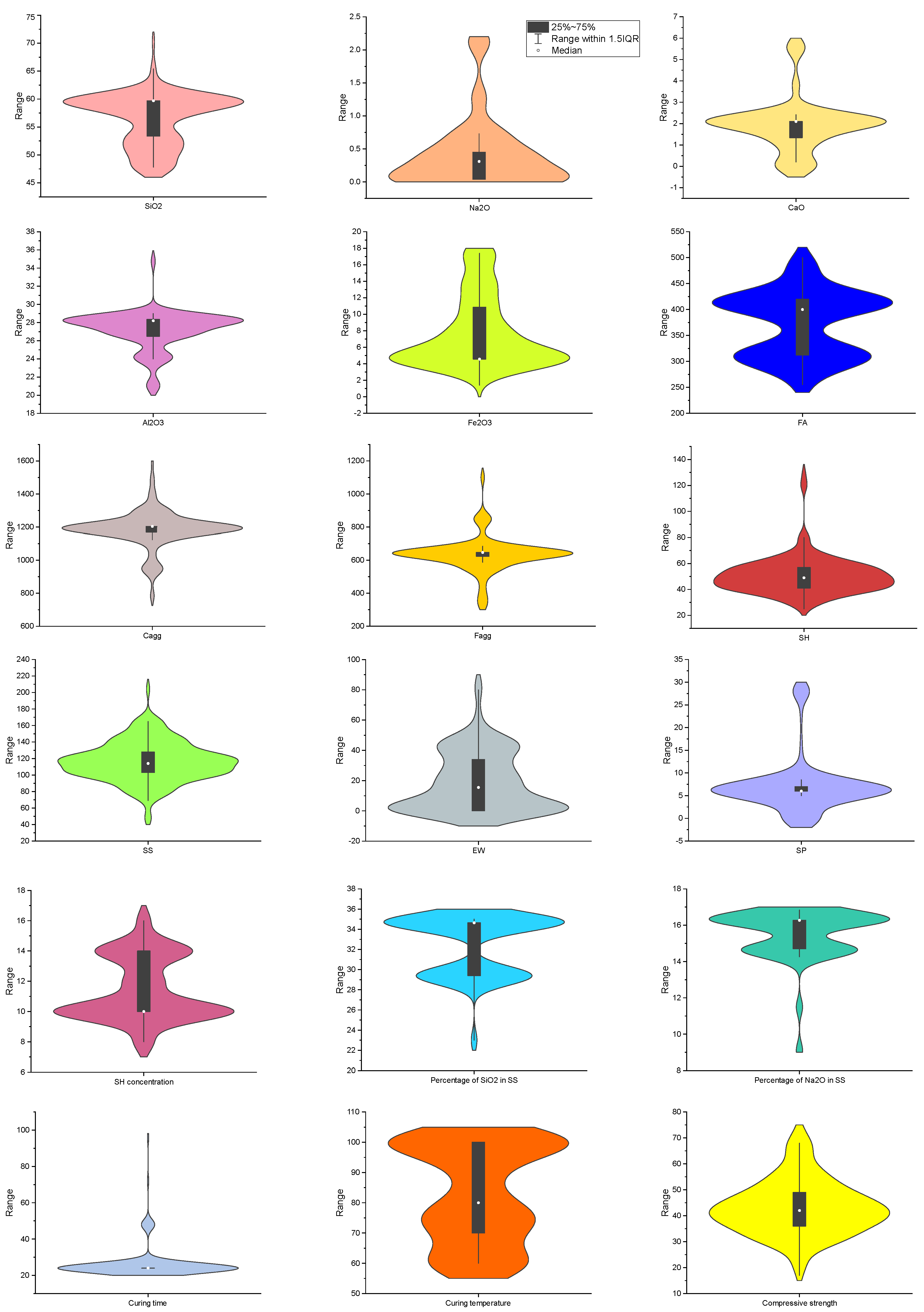
| Parameters | Symbol | Unit | Mean | Median | StD | Kurtosis | Skewness | Min | Max |
|---|---|---|---|---|---|---|---|---|---|
| * Percentage of SiO2 | SiO2 | % | 56.49 | 59.70 | 4.59 | −0.46 | −0.50 | 47.80 | 70.30 |
| * Percentage of Na2O | Na2O | % | 0.41 | 0.31 | 0.54 | 3.71 | 2.02 | 0.04 | 2.12 |
| * Percentage of CaO | CaO | % | 1.95 | 2.10 | 1.23 | 2.69 | 1.12 | 0.03 | 5.57 |
| * Percentage of Al2O3 | Al2O3 | % | 27.14 | 28.21 | 2.09 | 3.17 | −0.78 | 20.70 | 34.75 |
| * Percentage of Fe2O3 | Fe2O3 | % | 7.77 | 4.57 | 4.29 | −0.12 | 1.08 | 1.40 | 17.40 |
| Fly Ash | FA | kg/m3 | 372.68 | 400.00 | 62.81 | −1.13 | −0.06 | 255.00 | 500.00 |
| Coarse Aggregate | CAgg | kg/m3 | 1186.12 | 1204.00 | 109.03 | 3.71 | −0.59 | 785.00 | 1591.00 |
| Fine Aggregate | FAgg | kg/m3 | 633.26 | 647.00 | 107.65 | 5.27 | 0.51 | 318.00 | 1100.00 |
| Sodium Hydroxide solution | SH | kg/m3 | 50.63 | 49.00 | 14.46 | 10.22 | 2.40 | 25.00 | 129.00 |
| Sodium Silicate solution | SS | kg/m3 | 116.38 | 114.00 | 23.70 | 0.96 | 0.26 | 48.00 | 204.00 |
| Extra Water | EW | kg/m3 | 19.03 | 15.50 | 19.61 | 0.26 | 0.90 | 0.00 | 86.00 |
| Superplasticizer | SP | kg/m3 | 7.09 | 6.00 | 6.14 | 6.16 | 2.40 | 0.00 | 28.00 |
| SH concentration | SH | Molarity | 11.45 | 10.00 | 2.09 | −1.00 | 0.47 | 8.00 | 16.00 |
| Percentage of SiO2 in SS | - | % | 32.46 | 34.64 | 2.90 | −0.10 | −0.83 | 23.00 | 35.01 |
| Percentage of Na2O in SS | - | % | 15.52 | 16.27 | 1.37 | 8.12 | −2.37 | 9.10 | 16.84 |
| Curing time | - | h | 26.37 | 24.00 | 8.96 | 27.26 | 4.74 | 24.00 | 96.00 |
| Curing temperature | - | °C | 82.93 | 80.00 | 16.04 | −1.55 | −0.19 | 60.00 | 100.00 |
| Compressive strength | CS | MPa | 43.14 | 42.00 | 10.57 | 0.39 | 0.52 | 17.00 | 74.00 |
Disclaimer/Publisher’s Note: The statements, opinions and data contained in all publications are solely those of the individual author(s) and contributor(s) and not of MDPI and/or the editor(s). MDPI and/or the editor(s) disclaim responsibility for any injury to people or property resulting from any ideas, methods, instructions or products referred to in the content. |
© 2024 by the authors. Licensee MDPI, Basel, Switzerland. This article is an open access article distributed under the terms and conditions of the Creative Commons Attribution (CC BY) license (https://creativecommons.org/licenses/by/4.0/).
Share and Cite
Shi, X.; Chen, S.; Wang, Q.; Lu, Y.; Ren, S.; Huang, J. Mechanical Framework for Geopolymer Gels Construction: An Optimized LSTM Technique to Predict Compressive Strength of Fly Ash-Based Geopolymer Gels Concrete. Gels 2024, 10, 148. https://doi.org/10.3390/gels10020148
Shi X, Chen S, Wang Q, Lu Y, Ren S, Huang J. Mechanical Framework for Geopolymer Gels Construction: An Optimized LSTM Technique to Predict Compressive Strength of Fly Ash-Based Geopolymer Gels Concrete. Gels. 2024; 10(2):148. https://doi.org/10.3390/gels10020148
Chicago/Turabian StyleShi, Xuyang, Shuzhao Chen, Qiang Wang, Yijun Lu, Shisong Ren, and Jiandong Huang. 2024. "Mechanical Framework for Geopolymer Gels Construction: An Optimized LSTM Technique to Predict Compressive Strength of Fly Ash-Based Geopolymer Gels Concrete" Gels 10, no. 2: 148. https://doi.org/10.3390/gels10020148