Latent Abstractions in Generative Diffusion Models

Abstract

In this work, we study how diffusion-based generative models produce high-dimensional data, such as images, by relying on latent abstractions that guide the generative process. We introduce a novel theoretical framework extending Nonlinear Filtering (NLF), offering a new perspective on SDE-based generative models. Our theory is based on a new formulation of joint (state and measurement) dynamics and an information-theoretic measure of state influence on the measurement process. We show that diffusion models can be interpreted as a system of SDE, describing a non-linear filter where unobservable latent abstractions steer the dynamics of an observable measurement process. Additionally, we present an empirical study validating our theory and supporting previous findings on the emergence of latent abstractions at different generative stages.

1. Introduction

Generative models have become a cornerstone of modern machine learning, offering powerful methods for synthesizing high-quality data across various domains such as image and video synthesis [1,2,3], natural language processing [4,5,6,7], audio generation [8,9], and molecular structures and general 3D shapes [10,11,12,13], to name a few. These models transform an initial distribution, which is simple to sample from, into one that approximates the data distribution. Among these, diffusion-based models designed through the lenses of Stochastic Differential Equations (SDEs) [14,15,16] have gained popularity due to their ability to generate realistic and diverse data samples through a series of stochastic transformations.

In such models, the data generation process, as described by a substantial body of empirical research [17,18,19], appears to develop according to distinct stages: high-level semantics emerge first, followed by the incorporation of low-level details, culminating in a refinement (denoising) phase. Despite ample evidence, a comprehensive theoretical framework for modeling these dynamics remains underexplored.

Indeed, despite recent work on SDE-based generative models, refs. [20,21,22,23] shedding new light on such models, they fall short of explicitly investigating the emergence of abstract representations in the generative process. We address this gap by establishing a new framework for elucidating how generative models construct and leverage latent abstractions, approached through the paradigm of NLF [24,25,26].

NLF is used across diverse engineering domains [24], as it provides robust methodologies for the estimation and prediction of a system’s state amidst uncertainty and noise. NLF enables the inference of dynamic latent variables that define the system state based on observed data, offering a Bayesian interpretation of state evolution and the ability to incorporate stochastic system dynamics. The problem we consider is the following: an unobservable random variable X is measured through a noisy continuous-time process $Y_t$, wherein the influence of X on the noisy process is described by an observation function H, with the noise component modeled as a Brownian motion term. The goal is to estimate the a posteriori measure ${\pi }_t$ of the variable X given the entire historical trajectory of the measurement process $Y_t$.

In this work, we establish a connection between SDE-based generative models and NLF by observing that they can be interpreted as simulations of NLF dynamics. In our framework, the latent abstraction, which corresponds to certain real-world properties within the scope of classical nonlinear filtering and remains unaffected in a causal manner by the posterior process ${\pi }_t$, is implicitly simulated and iteratively refined. We explore the connection between latent abstractions and the a posteriori process, through the concept of filtrations—broadly defined as collections of progressively increasing information sets—and offer a rigorous theory to study the emergence and influence of latent abstractions throughout the data generation process. To ground the reader’s intuition in a concrete example, our experimental validation considers a scenario where latent abstractions correspond to scene descriptions—such as color, shape, and object size—that are subsequently rendered using a computer program.

Our theoretical contributions unfold as follows. In Section 2 we show how to reformulate classical NLF results such that the measurement process is the only available information, and derive the corresponding dynamics of both the latent abstraction and the measurement process. These results are summarized in Theorems 2 and 3.

Given the new dynamics, in Theorem 4, we show how to estimate the a posteriori measure of the NLF model and present a novel derivation to compute the mutual information between the measurement process and random variables derived from a transformation of the latent abstractions in Theorem 5. Finally, we show in Theorem 6 that the a posteriori measure is a sufficient statistic for any random variable derived from the latent abstractions when only having access to the measurement process.

Building on these general results, in Section 3 we present a novel perspective on continuous-time score-based diffusion models, which is summarised in Equation (10). We propose to view such generative models as NLF simulators that progress in two stages: first, our model updates the a posteriori measure representing sufficient statistics of the latent abstractions; second, it uses a projection of the a posteriori measure to update the measurement process. Such intuitive understanding is the result of several fundamental steps. In Theorems 7 and 8, we show that the common view of score-based diffusion models by which they evolve according to forward (noising) and backward (generative) dynamics is compatible with the NLF formulation, in which there is no need to distinguish between such phases. In other words, the NLF perspective of Equation (10) is a valid generative model. In Appendix H, we provide additional results (see Lemma A1), focusing on the specific case of linear diffusion models, which are the most popular instance of score-based generative models in use today. In Section 4, we summarize the main intuitions behind our NLF framework.

Our results explain, by means of a theoretically sound framework, the emergence of latent abstractions that has been observed by a large body of empirical work [17,18,19,27,28,29,30,31,32,33]. The closest research to our findings are discussed in [34,35,36], albeit from a different mathematical perspective. To root our theoretical results in additional empirical evidence, we conclude our work in Section 5 with a series of experiments on score-based generative models [14], where we (1) validate existing probing techniques to measure the emergence of latent abstractions, (2) compute the mutual information as derived in our framework and show that it is a suitable approach to measure the relation between the generative process and latent abstractions, and (3) introduce a new measurement protocol to further confirm the connections between our theory and how practical diffusion-based generative models operate.

2. Nonlinear Filtering

Consider two random variables $Y_t$ and X, corresponding to a stochastic measurement process ($Y_t$) of some underlying latent abstraction (X). We construct our universe sample space $\Omega$ as the combination of the space of continuous functions in the interval $[0,T]$ (i.e., $\mathcal{C}([0,T],{\mathbb{R}}^N)$ with $T\in {\mathbb{R}}^{+}$), and of a complete separable metric space $\mathcal{S}$, i.e., $\Omega =\mathcal{C}([0,T],{\mathbb{R}}^N)\times \mathcal{S}$. On this space, we consider the joint canonical process $Z_t\left(\omega \right)=[Y_t,X]=[{\omega }_t^y,{\omega }^x]$ for all $\omega \in \Omega$, with $\omega =[{\omega }^y,{\omega }^x]$. In this work, we indicate with $\sigma (·)$ sigma-algebras. Consider the growing filtration naturally induced by the canonical process ${\mathcal{F}}_t^{Y,X}=\sigma (Y_{0\le s\le t},X)$ (a short-hand for $\sigma (\sigma \left(Y_{0\le s\le t}\right)\cup \sigma \left(X\right))$), and define $\mathcal{F}={\mathcal{F}}_T^{Y,X}$. We build the probability triplet $(\Omega ,\mathcal{F},\mathrm{P})$, where the probability measure $\mathrm{P}$ is selected such that the process $\{Z_{0\le t\le T},{\mathcal{F}}_{0\le t\le T}^{Y,X}\}$ has the following SDE representation

$$Y_t=Y_0+{\int }_0^{t}H(Y_s,X,s)\mathrm{d}s+W_t,$$

(1)

where $\{W_{0\le t\le T},{\mathcal{F}}_{0\le t\le T}^{Y,X}\}$ is a Brownian motion with initial value 0 and $H:\Omega \times [0,T]\to {\mathbb{R}}^N$ is an observation process. All standard technical assumptions are available in Appendix A.

Next, we provide the necessary background on NLF, to pave the way for understanding its connection with the generative models of interest. The most important building block of the NLF literature is represented by the conditional probability measure $\mathrm{P}[X\in A|{\mathcal{F}}_t^Y]$ (notice the reduced filtration ${\mathcal{F}}_t^Y\subset {\mathcal{F}}_t^{Y,X}$), which summarizes, a posteriori, the distribution of X given observations of the measurement process until time t, that is, $Y_{0\le s\le t}$.

Theorem 1 

(Thm 2.1 [24]). Consider the probability triplet $(\Omega ,\mathcal{F},\mathrm{P})$, the metric space $\mathcal{S}$ and its Borel sigma-algebra $\mathcal{B}\left(\mathcal{S}\right)$. There exists a (probability measure valued $\mathcal{P}\left(\mathcal{S}\right)$) process $\{{\pi }_{0\le t\le T},{\mathcal{F}}_{0\le t\le T}^Y\}$, with a progressively measurable modification, such that for all $A\in \mathcal{B}\left(\mathcal{S}\right)$, the conditional probability measure $\mathrm{P}[X\in A|{\mathcal{F}}_t^Y]$ is well defined and is equal to ${\pi }_t\left(A\right)$.

The conditional probability measure is extremely important, as the fundamental goal of nonlinear filtering is the solution to the following problem. Here, we introduce the quantity $\varphi$, which is a random variable derived from the latent abstractions X.

Problem 1. 

For any fixed $\varphi :\mathcal{S}\to \mathbb{R}$ bounded and measurable, given knowledge of the measurement process $Y_{0\le s\le t}$, compute ${\mathbb{E}}_{\mathrm{P}}\left[\varphi \left(X\right)\right|{\mathcal{F}}_t^Y]$. This amounts to computing

$$\langle {\pi }_t,\varphi \rangle ={\int }_{\mathcal{S}}\varphi \left(x\right)\mathrm{d}{\pi }_t\left(x\right).$$

(2)

In simple terms, Problem 1 involves studying the existence of the a posteriori measure and the implementation of efficient algorithms for its update, using the flowing stream of incoming information $Y_t$. We first focus our attention on the existence of an analytic expression for the value of the a posteriori expected measure ${\pi }_t$. Then, we quantify the interaction dynamics between observable measurements and $\varphi$, through the lenses of mutual information $\mathcal{I}(Y_{0\le s\le t};\varphi )$, which is an extension of the problems considered in [37,38,39,40].

2.1. Technical Preliminaries

We set the stage of our work by revisiting the measurement process $Y_t$, and express it in a way that does not require access to unobservable information. Indeed, while $Y_t$ is naturally adapted with reference to its own filtration ${\mathcal{F}}_t^Y$, and consequently to any other growing filtration ${\mathcal{R}}_t$ such ${\mathcal{F}}_t^{Y,X}\supseteq {\mathcal{R}}_t\supseteq {\mathcal{F}}_t^Y$, the representation in Equation (1) is in general not adapted, letting aside degenerate cases.

Let us consider the family of growing filtrations ${\mathcal{R}}_t=\sigma ({\mathcal{R}}_0\cup \sigma (Y_{0\le s\le t}-Y_0))$, where $\sigma \left(Y_0\right)\subseteq {\mathcal{R}}_0\subseteq \sigma (X,Y_0)$. Intuitively, ${\mathcal{R}}_0$ allows to modulate between the two extreme cases of knowing only the initial conditions of the SDE, that is $Y_0$, to the case of complete knowledge of the whole latent abstraction X, and anything in between. As shown hereafter, the original process $Y_t$ associated with the space $(\Omega ,\mathcal{F},\mathrm{P})$ which solves Equation (1), also solves Equation (4), which is adapted on the reduced filtration ${\mathcal{R}}_t$. This allows us to reason about the partial observation of the latent abstraction (${\mathcal{R}}_0$ vs. $\sigma (X,Y_0)$), without incurring in the problem of the measurement process $Y_t$ being statistically dependent of the whole latent abstraction X.

Armed with such representation, we study under which change of measure the process $Y_t-Y_0$ behaves as a Brownian motion (Theorem 3). This serves the purpose of simplifying the calculation of the expected value of $\varphi$ given $Y_t$, as described in Problem 1. Indeed, if $Y_t-Y_0$ is a Brownian motion independent of $\varphi$, its knowledge does not influence our best guess for $\varphi$, i.e., the conditional expected value. Moreover, our alternative representation is instrumental for the efficient and simple computation of the mutual information $\mathcal{I}(Y_{0\le s\le t};\varphi )$, where the different measures involved in the Radon–Nikodym derivatives will be compared against the same reference Brownian measures.

The first step to define our representation is provided by the following

Theorem 2. 

[Appendix B] Consider the the probability triplet $(\Omega ,\mathcal{F},\mathrm{P})$, the process in Equation (1) defined on it, and the growing filtration ${\mathcal{R}}_t=\sigma ({\mathcal{R}}_0\cup \sigma (Y_{0\le s\le t}-Y_0))$. Define a new stochastic process

$$W_t^{\mathcal{R}}\stackrel{\mathit{def}}{=}{Y}_t-Y_0-{\int }_0^t{\mathbb{E}}_{\mathrm{P}}\left(H(Y_s,X,s)\right|{\mathcal{R}}_s)\mathrm{d}s.$$

(3)

Then, $\{W_{0\le t\le T}^{\mathcal{R}},{\mathcal{R}}_{0\le t\le T}\}$ is a Brownian motion. Notice that if ${\mathcal{R}}_t={\mathcal{F}}_t^{Y,X}$, then $W_t^{\mathcal{R}}=W_t$.

Following Theorem 2, the process $\{Y_{0\le t\le T},{\mathcal{R}}_{0\le t\le T}\}$ has SDE representation

$$Y_t=Y_0+{\int }_0^t{\mathbb{E}}_{\mathrm{P}}\left(H(Y_s,X,s)\right|{\mathcal{R}}_s)\mathrm{d}s+W_t^{\mathcal{R}}.$$

(4)

Next, we derive the change of measure necessary for the process ${\tilde{W}}_t\stackrel{\mathrm{def}}{=}{Y}_t-Y_0$ to be a Brownian motion with reference to to the filtration ${\mathcal{R}}_t$. To carry this out, we apply the Girsanov theorem [41] to ${\tilde{W}}_t$, which, in general, admits a $\mathcal{R}$-adapted representation ${\int }_0^t{\mathbb{E}}_{\mathrm{P}}\left(H(Y_s,X,s)\right|{\mathcal{R}}_s)\mathrm{d}s+W_t^{\mathcal{R}}$.

Theorem 3. 

[Appendix C] Define the new probability space $(\Omega ,{\mathcal{R}}_T,{\mathrm{Q}}^{\mathcal{R}})$ via the measure ${\mathrm{Q}}^{\mathcal{R}}\left(A\right)={\mathbb{E}}_{\mathrm{P}}\left[\mathbf{1}\left(A\right){\left({\psi }_T^{\mathcal{R}}\right)}^{-1}\right]$, for $A\in {\mathcal{R}}_T$, where

$${\psi }_t^{\mathcal{R}}\stackrel{\mathit{def}}{=}exp({\int }_0^t{\mathbb{E}}_{\mathrm{P}}\left[H(Y_s,X,s)\right|{\mathcal{R}}_s]\mathrm{d}{Y}_s-{\displaystyle \frac{1}{2}}{\int }_0^t{\left|\right|{\mathbb{E}}_{\mathrm{P}}\left[H(Y_s,X,s)\right|{\mathcal{R}}_s\left]\right||}^2\mathrm{d}s),$$

(5)

and

$${\mathrm{Q}}^{\mathcal{R}}{|}_{{\mathcal{R}}_t}={\mathbb{E}}_{\mathrm{P}}\left[\mathbf{1}\left(A\right){\mathbb{E}}_{\mathrm{P}}\left[{\left({\psi }_T^{\mathcal{R}}\right)}^{-1}\right|{\mathcal{R}}_t]\right]={\mathbb{E}}_{\mathrm{P}}\left[\mathbf{1}\left(A\right){\left({\psi }_t^{\mathcal{R}}\right)}^{-1}\right].$$

Then, the stochastic process $\{{\tilde{W}}_{0\le t\le T},{\mathcal{R}}_{0\le t\le T}\}$ is a Brownian motion on the space $(\Omega ,{\mathcal{R}}_T,{\mathrm{Q}}^{\mathcal{R}})$.

A direct consequence of Theorem 3 is that the process ${\tilde{W}}_t$ is independent of any ${\mathcal{R}}_0$ measurable random variable under the measure ${\mathrm{Q}}^{\mathcal{R}}$. Moreover, it holds that for all ${\mathcal{R}}_t^{\prime }\subseteq {\mathcal{R}}_t$, ${\mathrm{Q}}^{\mathcal{R}}{|}_{{\mathcal{R}}_t^{\prime }}={\mathrm{Q}}^{{\mathcal{R}}^{\prime }}{|}_{{\mathcal{R}}_t^{\prime }}$.

2.2. A Posteriori Measure and Mutual Information

As in Section 2 for the process ${\pi }_t$, here, we introduce a new process ${\pi }_t^{\mathcal{R}}$, which represents the conditional law of X given the filtration ${\mathcal{R}}_t=\sigma ({\mathcal{R}}_0\cup \sigma (Y_{0\le s\le t}-Y_0))$. More precisely, for all $A\in \mathcal{B}\left(\mathcal{S}\right)$, the conditional probability measure $\mathrm{P}[X\in A|{\mathcal{R}}_t]$ is well defined and is equal to ${\pi }_t^{\mathcal{R}}\left(A\right)$. Moreover, for any $\varphi :\mathcal{S}\to \mathbb{R}$ bounded and measurable, ${\mathbb{E}}_{\mathrm{P}}\left[\varphi \left(X\right)\right|{\mathcal{R}}_t]=\langle {\pi }_t^{\mathcal{R}},\varphi \rangle$. Notice that if $\mathcal{R}={\mathcal{F}}^Y$ then ${\pi }^{\mathcal{R}}$ reduces to $\pi$.

Armed with Theorem 3, we are ready to derive the expression for the a posteriori measure ${\pi }_t^{\mathcal{R}}$ and the mutual information between observable measurements and the unavailable information about the latent abstractions, that materialize in the random variable $\varphi$.

Theorem 4. 

[Appendix D] The measure-valued process ${\pi }_t^{\mathcal{R}}$ solves in weak sense (see Appendix D for a precise definition) the following SDE

$${\pi }_t^{\mathcal{R}}={\pi }_0^{\mathcal{R}}+{\int }_0^t{\pi }_s^{\mathcal{R}}\left(H(Y_s,·,s)-\langle {\pi }_s^{\mathcal{R}},H(Y_s,·,s)\rangle \right)\left(\mathrm{d}{Y}_s-\langle {\pi }_s^{\mathcal{R}},H(Y_s,·,s)\rangle \mathrm{d}s\right),$$

(6)

where the initial condition ${\pi }_0$ satisfies ${\pi }_0^{\mathcal{R}}\left(A\right)=\mathrm{P}[X\in A|{\mathcal{R}}_0]$ for all $A\in \mathcal{B}\left(\mathcal{S}\right)$.

When $\mathcal{R}={\mathcal{F}}^Y$, Equation (6) is the well-known Kushner–Stratonovitch (or Fujisaki—Kallianpur–Kunita) equation (see, e.g., [24]). A proof for uniqueness of the solution of Equation (6) can be approached by considering the strategies in [42], but is outside the scope of this work. The (recursive) expression in Equation (6) is particularly useful for engineering purposes since, in general, it is usually not known in which variables $\varphi \left(X\right)$, representing latent abstractions, we could be interested in. Keeping track of the whole distribution ${\pi }_t^{\mathcal{R}}$ at time t is the most cost-effective solution, as we will show later.

Our next goal is to quantify the interaction dynamics between observable measurements and latent abstractions that materialize through the variable $\varphi \left(X\right)$ (from now on, we write only $\varphi$ for the sake of brevity); in Theorem 5, we derive the mutual information $\mathcal{I}(Y_{0\le s\le t};\varphi )$.

Theorem 5. 

[Appendix E] The mutual information between observable measurements $Y_{0\le s\le t}$ and ϕ is defined as:

$$\mathcal{I}(Y_{0\le s\le t};\varphi )\stackrel{\mathit{def}}{=}\int log{\displaystyle \frac{{\mathrm{d}\mathrm{P}}_{\#Y_{0\le s\le t},\varphi }}{{\mathrm{d}\mathrm{P}}_{\#Y_{0\le s\le t}}{\mathrm{d}\mathrm{P}}_{\#\varphi }}}{\mathrm{d}\mathrm{P}}_{\#Y_{0\le s\le t},\varphi }.$$

(7)

It holds that such quantity is equal to ${\mathbb{E}}_{\mathrm{P}}\left[log{\displaystyle \frac{\mathrm{d}\mathrm{P}{|}_{{\mathcal{R}}_t}}{\mathrm{d}\mathrm{P}{|}_{{\mathcal{F}}_t^Y}\mathrm{d}\mathrm{P}{|}_{\sigma \left(\varphi \right)}}}\right]$, with ${\mathcal{R}}_t=\sigma (Y_{0\le s\le t},\varphi )$, which can be simplified as follows:

$$\mathcal{I}(Y_0;\varphi )+{\displaystyle \frac{1}{2}}{\mathbb{E}}_{\mathrm{P}}\left[{\int }_0^t{\left|\right|{\mathbb{E}}_{\mathrm{P}}\left[H(X,Y_s,s)\right|{\mathcal{F}}_s^Y]-{\mathbb{E}}_{\mathrm{P}}\left[H(X,Y_s,s)\right|{\mathcal{R}}_s\left]\right||}^2\mathrm{d}s\right].$$

(8)

The mutual information computed by Equation (8) is composed of two elements: first, the mutual information between the initial measurements $Y_0$ and $\varphi$, which is typically zero by construction. The second term quantifies how much the best prediction of the observation function H is influenced by the extra knowledge of $\varphi$, in addition to the measurement history $Y_{0\le s\le t}$. By adhering to the premise that the conditional expectation of a stochastic variable constitutes the optimal estimator given the conditioning information, the integral on the right-hand side quantifies the expected squared difference between predictions, having access to measurements only (${\mathbb{E}}_{\mathrm{P}}[·|{\mathcal{F}}_t^Y]$) and those incorporating additional information (${\mathbb{E}}_{\mathrm{P}}[·|{\mathcal{R}}_t]$).

Even though a precise characterization for general observation functions and and variables $\varphi$ is typically out of reach, a qualitative analysis is possible. First, the mutual information between $\varphi$ and the measurements depends on (i) how much the amplitude of H is impacted by knowledge of $\varphi$ and (ii) the number of elements of H that are impacted (informally, how much localized vs. global is the impact of $\varphi$). Second, it is possible to define a hierarchical interpretation about the emergence of the various latent factors: a variable with a local impact can “appear”, in an information theoretic sense, only if the impact of other global variables is resolved; otherwise, the remaining uncertainty of the global variables makes knowledge of the local variable irrelevant. In classical diffusion models, this is empirically known [17,18,19], and corresponds to the phenomenon where semantics emerges before details (global vs. local details in our language). For instance, as shown in Section 5, during the generative dynamics, latent abstractions which correspond to high level properties such as color and geometric aspect ratio emerge in very early stages of the process.

Now, consider any ${\mathcal{F}}_t^Y$ measurable random variable ${\tilde{Y}}_t$, defined as a mapping to a generic measurable space $(\Psi ,\mathcal{B}(\Psi \left)\right)$, which means it can also be seen as a process. The data processing inequality states that the mutual information between such $\tilde{Y}$ and $\varphi$ will be smaller than the mutual information between the original measurement process and $\varphi$. However, it can be shown that all the relevant information about the random variable $\varphi$ contained in ${\mathcal{F}}_t^Y$ is equivalently contained in the filtering process at time instant t, that is ${\pi }_t$. This is not trivial, since ${\pi }_t$ is a ${\mathcal{F}}_t^Y$-measurable quantity, i.e., $\sigma \left({\pi }_t\right)\subset {\mathcal{F}}_t^Y$. In other words, we show that ${\pi }_t$ is a sufficient statistic for any $\sigma \left(X\right)$ measurable random variable when starting from the measurement process.

Theorem 6. 

[Appendix F] For any ${\mathcal{F}}_t^Y$ measurable random variable ${\tilde{Y}}_t:\Omega \to \Psi$, the following inequality holds:

$$\mathcal{I}(\tilde{Y};\varphi )\le \mathcal{I}(Y_{0\le s\le t};\varphi ).$$

(9)

For a given $t\ge 0$, the measurement process $Y_{0\le s\le t}$ and X are conditionally-independent given ${\pi }_t$. This implies that $\mathrm{P}\left(A\right|\sigma \left({\pi }_t\right))=\mathrm{P}\left(A\right|{\mathcal{F}}_t^Y),\forall A\in \sigma \left(X\right)$. Then, $\mathcal{I}(Y_{0\le s\le t};\varphi )=\mathcal{I}({\pi }_t;\varphi )$ (i.e., Equation (9) is attained with equality).

While ${\pi }_t$ contains all the relevant information about $\varphi$, the same cannot be said about the conditional expectation, i.e., the particular case $\tilde{Y}=\langle {\pi }_t,\varphi \rangle$. Indeed, from Equation (2), $\langle {\pi }_t,\varphi \rangle$ is obtained as a transformation of ${\pi }_t$ and thus can be interpreted as a ${\mathcal{F}}_t^Y$ measurable quantity subject to the constraint of Equation (9). As a particular case, the quantity $\langle {\pi }_t,H\rangle$, of central importance in the construction of generative models Section 3, carries, in general, less information about $\varphi$ than the un-projected ${\pi }_t$.

3. Generative Modeling

We are interested in generative models for a given $\sigma \left(X\right)$-measurable random variable V. An intuitive illustration of how data generation works according to our framework is as follows. Consider, for example, the image domain, and the availability of a rendering engine that takes as an input a computer program describing a scene (coordinates of objects, textures, light sources, auxiliary labels, etc...) and that produces an output image of the scene. In a similar vein, a generative model learns how to use latent variables (which are not explicitly provided in input, but rather implicitly learned through training) to generate an image. For such a model to work, one valid strategy is to consider an SDE in the form of Equation (1) where the following holds (from a strictly technical point of view, Assumption 1 might be incompatible with other assumptions in Appendix A, or proving compatibility could require particular effort. Such details are discussed in Appendix G).

Assumption 1. 

The stochastic process $Y_t$ satisfies $Y_T=V,\mathrm{P}-a.s.$

Then, we could numerically simulate the dynamics of Equation (1) until time T. Indeed, starting from initial conditions $Y_0$, we could obtain $Y_T$ that, under Assumption 1, is precisely V. Unfortunately, such a simple idea requires explicit access to X, as it is evident from Equation (1). In mathematical terms, Equation (1) is adapted to the filtration ${\mathcal{F}}_t^{Y,X}$. However, we have shown how to reduce the available information to account only for historical values of $Y_t$. Then, we can combine the result in Theorem 4 with Theorem 2 and re-interpret Equation (4), which is a valid generative model, as

$$\left\{\begin{array}{c}{\pi }_t={\pi }_0+{\int }_0^t{\pi }_s\left(H-\langle {\pi }_s,H\rangle \right)\left(\mathrm{d}{Y}_s-\langle {\pi }_s,H\rangle \mathrm{d}s\right),\hfill \\ Y_t=Y_0+{\int }_0^t\langle {\pi }_s,H\rangle \mathrm{d}s+W_t^{{\mathcal{F}}^Y},\hfill \end{array}\right.$$

(10)

where H denotes $H(Y_s,·,s)$. Explicit simulation of Equation (10) only requires knowledge of the whole history of the measurement process: provided Assumption 1 holds, it allows generation of a sample of the random variable V.

Although the discussion in this work includes a large class of observation functions, we focus on the particular case of generative diffusion models [14]. Typically, such models are presented through the lenses of a forward noising process and backward (in time) SDEs, following the intuition of Anderson [43]. Next, according to the framework we introduce in this work, we reinterpret such models from the perspective of enlargement of filtrations.

Consider the reversed process ${\widehat{Y}}_t\stackrel{\mathrm{def}}{=}{Y}_{T-t}$ defined on $(\Omega ,\mathcal{F},\mathrm{P})$ and the corresponding filtration ${\mathcal{F}}_t^{\widehat{Y}}\stackrel{\mathrm{def}}{=}\sigma \left({\widehat{Y}}_{0\le s\le t}\right)$. The measure $\mathrm{P}$ is selected such that the process ${\widehat{Y}}_t$ has a ${\mathcal{F}}_t^{\widehat{Y}}$-adapted expression

$${\widehat{Y}}_t=V+\underset{0}{\overset{t}{\int }}F({\widehat{Y}}_s,s)\mathrm{d}s+{\widehat{W}}_t,$$

(11)

where $\{{\widehat{W}}_t,{\mathcal{F}}_t^{\widehat{Y}}\}$ is a Brownian motion. Then, Assumption 1 is valid since $Y_T={\widehat{Y}}_0=V$. Note that Equation (11), albeit with a different notation, is reminiscent of the forward SDE that is typically used as the starting point to illustrate score-based generative models [14]. In particular, $F(·)$ corresponds to the drift term of such a diffusion SDE.

Equation (11) is equivalent to $Y_t=V+\underset{t}{\overset{T}{\int }}F(Y_s,T-s)\mathrm{d}s+{\widehat{W}}_{T-t}$, which is an expression for the process $Y_t$, which is adapted to ${\mathcal{F}}^{\widehat{Y}}$. This constitutes the first step to derive an equivalent backward (generative) process according to the traditional framework of score-based diffusion models. Note that such an equivalent representation is not useful for simulation purposes: the goal of the next step is to transform it such that it is adapted to ${\mathcal{F}}^Y$. Indeed, using simple algebra, it holds that

$$Y_t=Y_0-\underset{0}{\overset{t}{\int }}F(Y_s,T-s)\mathrm{d}s+\left(-Y_0+V+\underset{0}{\overset{T}{\int }}F(Y_s,T-s)\mathrm{d}s+{\widehat{W}}_{T-t}\right),$$

where the last term in the parentheses is equal to $-{\widehat{W}}_T+{\widehat{W}}_{T-t}$.

Note that ${\mathcal{F}}_t^Y=\sigma \left({\widehat{Y}}_{T-t\le s\le T}\right)$. Since $\sigma \left({\widehat{Y}}_{T-t\le s\le T}\right)=\sigma \left({\widehat{W}}_{T-t\le s\le T}\right)\cup \sigma \left({\widehat{Y}}_{T-t}\right)$, we can apply the result in [44] (Thm 2.2) to claim the following: $-{\widehat{W}}_T+{\widehat{W}}_{T-t}-{\int }_0^t\nabla log\widehat{p}(Y_s,T-s)\mathrm{d}s$ is a Brownian motion adapted to ${\mathcal{F}}_t^Y$, where this time $\mathrm{P}({\widehat{Y}}_t\in \mathrm{d}y)=\widehat{p}(y,t)\mathrm{d}y$. Then, [44].

Theorem 7. 

Consider the stochastic process $Y_t$ which solves Equation (11). The same stochastic process also admits a ${\mathcal{F}}_t^Y$-adapted representation

$$Y_t=Y_0+{\int }_0^t\underset{\mathit{In}\mathit{Theorem}8,\mathit{we}\mathit{call}\mathit{this}{F}^{\prime }(Y_s,s)}{\underbrace{-F(Y_s,T-s)+\nabla log\widehat{p}(Y_s,T-s)}}\mathrm{d}s+W_t.$$

(12)

Equation (12) corresponds to the backward diffusion process from [14] and, because it is adapted to the filtration ${\mathcal{F}}^Y$, it represents a valid, and easy-to-simulate, measurement process.

By now, it is clear how to go from an ${\mathcal{F}}^{Y,X}$-adapted filtration to a ${\mathcal{F}}^Y$-adapted one. We also showed that a ${\mathcal{F}}^Y$-adapted filtration can be linked to the reverse, ${\mathcal{F}}^{\widehat{Y}}$-adapted process induced by a forward diffusion SDE. What remains to be discussed is the connection that exists between the ${\mathcal{F}}^Y$-adapted filtration, and its enlarged version ${\mathcal{F}}^{Y,X}$. In other words, we have shown that a forward, diffusion SDE admits a backward process which is compatible with our generative model that simulates a NLF process having access only to measurements, but we need to make sure that such process admits a formulation that is compatible with the standard NLF framework in which latent abstractions are available.

To carry this out, we can leverage existing results about Markovian bridges [22,45] (and further work [46,47,48,49] on filtration enlargement). This requires assumptions about the existence and well-behaved nature of densities $p(y,t)$ of the SDE process, defined by the logarithm of the Radon–Nikodym derivative of the instantaneous measure $\mathrm{P}(Y_t\in \mathrm{d}y)$ with reference to the Lebesgue measure in ${\mathbb{R}}^N$, $\mathrm{P}(Y_t\in \mathrm{d}y)=p(y,t)\mathrm{d}y$ (the analysis of the existence of the process adapted to ${\mathcal{F}}_t^Y$ is considered in the time interval $[0,T)$ [50]; see also Appendix G).

Theorem 8. 

Suppose that on $(\Omega ,\mathcal{F},\mathrm{P})$, the Markov stochastic process $Y_t$ satisfies

$$Y_t=Y_0+{\int }_0^t{F}^{\prime }(Y_s,s)\mathrm{d}s+W_t,$$

where $\{W_{0\le t\le T},{\mathcal{F}}_{0\le t\le T}^Y\}$ is a Brownian motion and F satisfies the requirements for existence and well definition of the stochastic integral [51]. Moreover, let Assumption 1 hold. Then, the same process admits ${\mathcal{R}}_t=\sigma (Y_{0\le s\le t},Y_T)$-adapted representation

$$Y_t=Y_0+{\int }_0^t{F}^{\prime }(Y_s,s)+{\nabla }_{Y_s}logp\left(Y_T\right|Y_s)\mathrm{d}s+{\beta }_t,$$

(13)

where $p\left(Y_T\right|Y_s)$ is the density with reference to the Lebesgue measure of the probability $\mathrm{P}\left(Y_T\right|\sigma \left(Y_s\right))$, and $\{{\beta }_{0\le t\le T},{\mathcal{R}}_{0\le t\le T}\}$ is a Brownian motion.

The connection between time reversal of diffusion processes and enlarged filtrations is finalized with the result of Al-Hussaini and Elliott [52], Thm. 3.3, where it is proved how the ${\beta }_t$ term of Equation (13) is a Brownian motion, using the techniques of time reversals of SDEs.

Since $\widehat{p}(y,T-t)=p(y,t)$, the enlarged filtration version of Equation (12) reads

$$Y_t=Y_0+{\int }_0^t\underset{\mathrm{Equivalent}\mathrm{to}H(Y_t,X,t)=-F(Y_s,T-s)+{\nabla }_{Y_s}logp\left(Y_s\right|V}{\underbrace{-F(Y_s,T-s)+{\nabla }_{Y_s}logp\left(Y_s\right|Y_T)\mathrm{d}s}}+W_t.$$

(14)

Note that the dependence of $Y_t$ on the latent abstractions X is implicitly defined by conditioning the score term ${\nabla }_{Y_s}logp\left(Y_s\right|Y_T)$ by $Y_T$, which is the “rendering” of X into the observable data domain.

Clearly, Equation (14) can be reverted to the starting generative Equation (12) by mimicking the results which allowed us to go from Equation (1) to Equation (4), by noticing that ${\mathbb{E}}_{\mathrm{P}}[{\nabla }_{Y_s}logp\left(Y_T\right|Y_s)|{\mathcal{F}}_t^Y]=0$ (informally, this is obtained since $\int {\nabla }_{y_s}logp\left(y_t\right|y_s)p\left(y_t\right|y_s)\mathrm{d}{y}_t=\int {\nabla }_{y_s}p\left(y_t\right|y_s)\mathrm{d}{y}_t=0$).

It is also important to notice that we can derive the expression for the mutual information between the measurement process and a sample from the data distribution, as follows

$$\mathcal{I}(Y_{0\le s\le t};V)=\mathcal{I}(Y_0;V)+{\displaystyle \frac{1}{2}}{\mathbb{E}}_{\mathrm{P}}\left[{\int }_0^t||{{\nabla }_{Y_s}logp\left(Y_s\right)-{\nabla }_{Y_s}logp\left(Y_s\right|Y_T)\left|\right|}^2\mathrm{d}s\right].$$

Mutual information is tightly related to the classical loss function of generative diffusion models.

Furthermore, by casting the result of Equation (8) according to the forms of Equations (12) and (14), we obtain the simple and elegant expression

$$\mathcal{I}(Y_{0\le s\le t};V)=\mathcal{I}(Y_0;V)+{\displaystyle \frac{1}{2}}{\mathbb{E}}_{\mathrm{P}}\left[{\int }_0^t{||{\nabla }_{Y_s}logp\left(Y_T\right|Y_s)||}^2\mathrm{d}s\right].$$

In Appendix H, we present a specialization of our framework for the particular case of linear diffusion models, recovering the expressions for the variance-preserving and variance-exploding SDEs that are the foundations of score-based generative models [14].

4. An Informal Summary of the Results

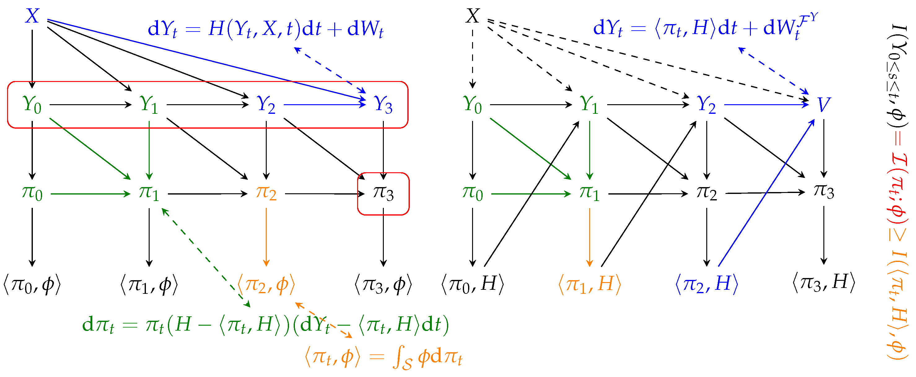
We shall now take a step back from the rigor of this work, and provide an intuitive summary of our results, using Figure 1 as a reference.

We begin with an illustration of NLF, shown on the left of the figure. We consider an observable latent abstraction X and the measurement process $Y_t$, which, for ease of illustration, we consider evolving in discrete time, i.e., $Y_0,Y_1,\cdots$, and whose joint evolution is described by Equation (1). Such an interaction is shown in blue: $Y_3$ depends on its immediate past $Y_2$ and the latent abstraction X.

The a posteriori measure process ${\pi }_t$ is updated in an iterative fashion by integrating the flux of information. We show this in green: ${\pi }_1$ is obtained by updating ${\pi }_0$ with $Y_1-Y_0$ (the equivalent of $\mathrm{d}{Y}_t$). This evolution is described by Kushner’s equation, which has been derived informally from the result of Equation (6). The a posteriori process is a sufficient statistic for the latent abstraction X: for example, ${\pi }_3$ contains the same information about $\varphi$ as the whole $Y_0,\cdots ,Y_3$ (red boxes). Instead, in general, a projected statistic $\langle {\pi }_t,\varphi \rangle$ contains less information than the whole measurement process (this is shown in orange, for time instant 2). The mutual information between all these variables is proven in Theorem 6, whereas the actual value of $\mathcal{I}(Y_{0\le s\le t};\varphi )$ is shown in Theorem 5.

Next, we focus on generative modeling. As per our definition, any stochastic process satisfying Assumption 1 ($Y_3=V$, in the figure) can be used for generative purposes. Since the latent abstraction is by definition not available, it is not possible to simulate directly the dynamics using Equation (1) (dashed lines from X to $Y_t$). Instead, we derive a version of the process adapted to the history of $Y_t$ alone, together with the update of the projection $\langle {\pi }_t,H\rangle$, which amounts to simulating Equation (10). In [36], diffusion models are shown to solve a “self-consistency” equation akin to a mean-field fixed point. Our framework aligns with this view by revealing how SDE-based generative processes implicitly enforce self-consistency between latent abstractions and measurements.

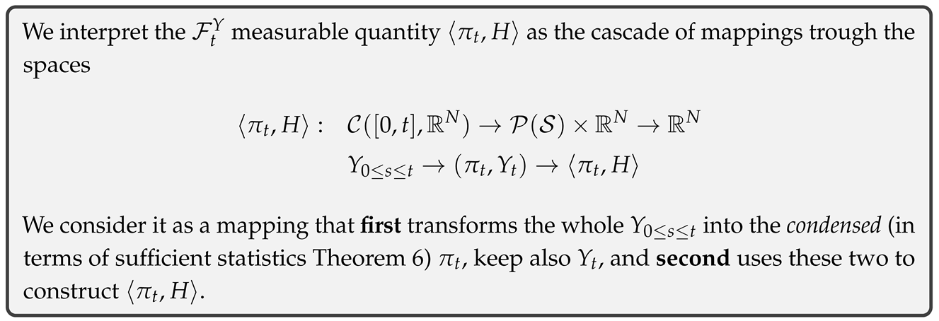
The update of the upper part of Equation (10), which is a particular case of Equation (6), can be interpreted as the composition of two steps: (1) (green) the update of the a posteriori measure given new available measurements, and, (2) (orange) the projection of the whole ${\pi }_t$ into the statistic of interest. The update of the measurement process, i.e., the lower part of Equation (10), is color-coded in blue. This is in stark contrast to the NLF case, as the update of, e.g., $Y_3=V$ does not depend directly on X. The system in Equation (10) and its simulation describes the emergence of latent world representations in SDE-based generative models:

The theory developed in this work guarantees that the mutual information between measurements and any statistics $\varphi$ grows as described by Theorem 5. Our framework offers a new perspective, according to which, the dynamics of SDE-based generative models [14] implicitly mimic the two steps procedure described in the box above. We claim that this is the reason why it is possible to dissect the parametric drift of such generative models and find a representation of the abstract state distribution ${\pi }_t$, encoded into their activations. Next, we set to root our theoretical findings in experimental evidence.

Generality of Our Framework

While previous works studied latent abstraction emergence specifically within diffusion-based generative models, our current theoretical framework deliberately transcends this scope. Indeed, the results presented in this paper can be interpreted as a generalization of the results contained in [53] (see also Equation (A10)) and apply broadly to any generative model satisfying Assumption 1. Such generality includes a wide variety of generative modeling techniques, such as Neural Stochastic Differential Equations (neural SDEs) [54], Schrödinger Bridges [55], and Stochastic Normalizing Flows [56]. In all these cases, our results on latent abstractions still hold; thus, the insights provided by our framework pave the way for deeper theoretical understanding and wider applicability across generative modeling paradigms.

5. Empirical Evidence

We complement existing empirical studies [17,18,19,30,31,32,33,34] that first measured the interactions between the generative process of diffusion models and latent abstractions, by focusing on a particular dataset that allows for a fine-grained assessment of the influence of latent factors.

Dataset. We use the Shapes3D [57] dataset, which is a collection of $64\times 64$ ray-tracing generated images, depicting simple 3D scenes, with an object (a sphere, cube,...) placed in a space, described by several attributes (color, size, orientation). Attributes have been derived from the computer program that the ray-tracing software executed to generate the scene: these are transformed into labels associated with each image. In our experiments, such labels are the materialization of the latent abstractions X we consider in this work (see Appendix J.1 for details).

Measurement Protocols. For our experiments, we use the base NCSPP model described by [14]: specifically, our denoising score network corresponds to a U-NET [58]. We train the unconditional version of this model from scratch using a score-matching objective. Detailed hyper-parameters and training settings are provided in Appendix J.2. Next, we summarize three techniques to measure the emergence of latent abstractions through the lenses of the labels associated with each image in our dataset. For all such techniques, we use a specific “measurement” subset of our dataset, which we partition in 246 training, 150 validation, and 371 test examples. We use a multi-label stratification algorithm [59,60] to guarantee a balanced distribution of labels across all dataset splits.

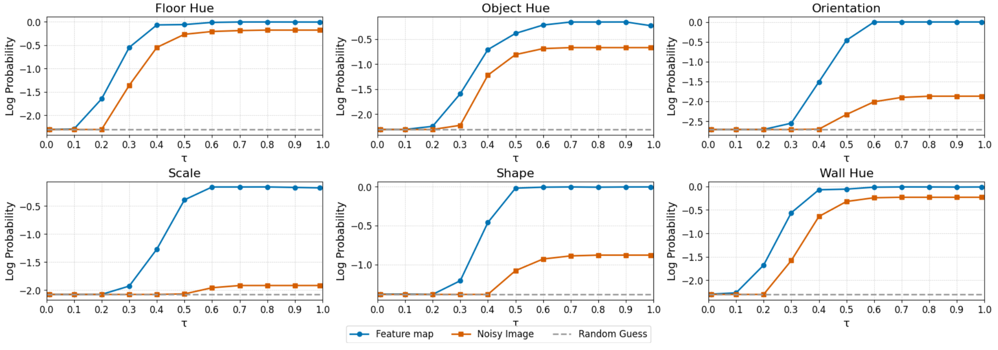
Linear probing. Each image in the measurement subset is perturbed with noise, using a variance-exploding schedule [14], with noise levels decreasing from $\tau =0$ to $\tau =1.0$ in steps of 0.1, as shown in Figure 2. Intuitively, each time value $\tau$ can be linked to a different signal-to-noise ratio ($SNR$), ranging from $SNR(\tau =1)=\infty$ to $SNR(\tau =0)\simeq 0$. We extract several feature maps from all the linear and convolutional layers of the denoising score network, for each perturbed image, resulting in a total of 162 feature map sets for each noise level. This process yields 11 different datasets per layer, which we use to train a linear classifier (our probe) for each of these datasets, using the training subset. In these experiments, we use a batch size of 64 and adjust the learning rate based on the noise level (see Appendix J.3). Classifier performance is optimized by selecting models based on their log-probability accuracy observed on the validation subset. The final evaluation of each classifier is conducted on the test subset. Classification accuracy, measured by the model log likelihood, is a proxy of latent abstraction emergence [17].

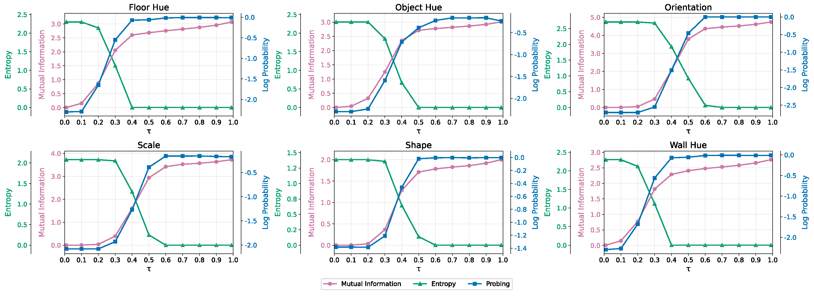
Mutual information estimation. We estimate mutual information between the labels and the outputs of the diffusion model across varying diffusion times, using Equation (A10) (which is a specialized version of our theory for linear diffusion models; see Appendix H) and adopt the same methodology discussed by Franzese et al. [53] to learn conditional and unconditional score functions and to approximate the mutual information. The training process uses a randomized conditioning scheme: 33% of training instances are conditioned on all labels, 33% on a single label, and the remaining 33% are trained unconditionally. See Appendix J.4 for additional details.

Forking. We propose a new technique to measure at which stage of the generative process, image features described by our labels emerge. Given an initial noise sample, we proceed with numerical integration of the backward SDE [14] up to time $\tau$. At this point, we fork k replicas of the backward process and continue the k generative pathways independently until numerical integration concludes. We use a simple classifier (a pre-trained ResNet50 [61] with an additional linear layer trained from scratch) to verify that labels are coherent across the k forks. Coherency is measured using the entropy of the label distribution output by our simple classifier on each latent factor for all the k branches of the fork. Intuitively, if we fork the process at time $\tau =0.6$, and the k forks all end up displaying a cube in the image (entropy equals 0), this implies that the object shape is a latent abstraction that has already emerged by time $\tau$. Conversely, lack of coherence implies that such a latent factor has not yet influenced the generative process. Details of the classifier training and sampling procedure are provided in Appendix J.5.

Results. We present our results in Figure 3. We note that some attributes like floor hue, wall hue and shape emerge earlier than others, which corroborates the hierarchical nature of latent abstractions, a phenomenon that is related to the spatial extent of each attribute in pixel space. This is evident from the results of linear probing, where we evaluate the performance of linear probes trained on features maps extracted from the denoiser network, and from the mutual information measurement strategy and the measured entropy of the predicted labels across forked generative pathways. Entropy decreases with $\tau$, which marks the moment in which the generative process proceeds along k forks. When generative pathways converge to a unique scene with identical predicted labels (entropy reaches zero), this means that the model has committed to a specific set of latent factors (breaking some of the symmetries in the language of [36]). This coincides with the same noise level corresponding to high accuracy for the linear probe, and high-values of mutual information. Further ablation experiments are presented in Appendix J.6.

6. Potential Applications and Practical Implications

Our theoretical analysis and experimental results provide a novel information-theoretic perspective on diffusion-based generative models. Besides the primary theoretical contribution, our framework naturally suggests several promising practical applications and implications. First, the explicit characterization of latent abstractions through mutual information measures may facilitate novel strategies for conditional generation, where generative processes could be guided or steered in a principled manner by explicitly controlling the latent abstraction process. Second, the insights derived from our nonlinear filtering viewpoint offer opportunities for enhanced interpretability and robustness in downstream applications that utilize learned latent representations, potentially leading to more reliable model behaviors. These practical implications represent compelling directions for future research, extending the reach and usability of diffusion-based generative modeling frameworks.

7. Conclusions

Despite their tremendous success in many practical applications, a deep understanding of how SDE-based generative models operate remained elusive. A particularly intriguing aspect of several empirical investigations was to uncover the capacity of generative models to create entirely new data by combining latent factors learned from examples. To the best of our knowledge, there exists no theoretical framework that attempts to describe such a phenomenon.

In this work, we closed this gap, and presented a novel theory—which builds on the framework of NLF—to describe the implicit dynamics allowing SDE-based generative models to tap into latent abstractions and guide the generative process. Our theory, which required advancing the standard NLF formulation, culminates in a new system of joint SDEs that fully describes the iterative process of data generation. Furthermore, we derived an information-theoretic measure to study the influence of latent abstractions, which provides a concrete understanding of the joint dynamics.

To root our theory into concrete examples, we collected experimental evidence by means of novel (and established) measurement strategies that corroborate our understanding of diffusion models. Latent abstractions emerge according to an implicitly learned hierarchy and can appear early on in the data generation process, much earlier than what is visible in the data domain. Our theory is especially useful as it allows analyses and measurements of generative pathways, opening up opportunities for a variety of applications, including image editing, and improved conditional generation.

References

1. Dhariwal, P.; Nichol, A. Diffusion Models Beat GANs on Image Synthesis. In Proceedings of the Advances in Neural Information Processing Systems, Online, 6–14 December 2021; Ranzato, M., Beygelzimer, A., Dauphin, Y., Liang, P., Vaughan, J.W., Eds.; Curran Associates, Inc.: Red Hook, NY, USA, 2021; Volume 34, pp. 8780–8794. [Google Scholar]
2. Ho, J.; Chan, W.; Saharia, C.; Whang, J.; Gao, R.; Gritsenko, A.; Kingma, D.P.; Poole, B.; Norouzi, M.; Fleet, D.J.; et al. Imagen Video: High Definition Video Generation with Diffusion Models. 2022. Available online: https://imagen.research.google/video/paper.pdf (accessed on 21 February 2025).
3. He, Y.; Yang, T.; Zhang, Y.; Shan, Y.; Chen, Q. Latent Video Diffusion Models for High-Fidelity Video Generation with Arbitrary Lengths. arXiv 2022, arXiv:2211.13221. [Google Scholar]
4. Li, X.L.; Thickstun, J.; Gulrajani, I.; Liang, P.; Hashimoto, T. Diffusion-LM Improves Controllable Text Generation. Oh, A.H., Agarwal, A., Belgrave, D., Cho, K., Eds.. In Proceedings of the Advances in Neural Information Processing Systems, New Orleans, LA, USA, 28 November–9 December 2022. [Google Scholar]
5. He, Z.; Sun, T.; Tang, Q.; Wang, K.; Huang, X.; Qiu, X. DiffusionBERT: Improving Generative Masked Language Models with Diffusion Models. In Proceedings of the 61st Annual Meeting of the Association for Computational Linguistics, Toronto, ON, Canada, 9–14 July 2023; Volume 1. Long Papers. [Google Scholar]
6. Gulrajani, I.; Hashimoto, T. Likelihood-Based Diffusion Language Models. In Proceedings of the Thirty-Seventh Conference on Neural Information Processing Systems, New Orleans, LA, USA, 10–16 December 2023. [Google Scholar]
7. Lou, A.; Meng, C.; Ermon, S. Discrete Diffusion Modeling by Estimating the Ratios of the Data Distribution. In Proceedings of the International Conference on Machine Learning, Vienna, Austria, 21–27 July 2024. [Google Scholar]
8. Kong, Z.; Ping, W.; Huang, J.; Zhao, K.; Catanzaro, B. DiffWave: A Versatile Diffusion Model for Audio Synthesis. In Proceedings of the International Conference on Learning Representations, Vienna, Austria, 4 May 2021. [Google Scholar]
9. Liu, J.; Li, C.; Ren, Y.; Chen, F.; Zhao, Z. DiffSinger: Singing Voice Synthesis via Shallow Diffusion Mechanism. Proc. AAAI Conf. Artif. Intell. 2022, 36, 11020–11028. [Google Scholar]
10. Trippe, B.L.; Yim, J.; Tischer, D.; Baker, D.; Broderick, T.; Barzilay, R.; Jaakkola, T. Diffusion probabilistic modeling of protein backbones in 3D for the motif-scaffolding problem. arXiv 2022, arXiv:2206.04119. [Google Scholar]
11. Hoogeboom, E.; Satorras, V.G.; Vignac, C.; Welling, M. Equivariant Diffusion for Molecule Generation in 3D. In Proceedings of the 39th International Conference on Machine Learning, Baltimore, MD, USA, 17–23 July 2022; Chaudhuri, K., Jegelka, S., Song, L., Szepesvari, C., Niu, G., Sabato, S., Eds.; Proceedings of Machine Learning Research. Volume 162, pp. 8867–8887. [Google Scholar]
12. Luo, S.; Hu, W. Diffusion Probabilistic Models for 3D Point Cloud Generation. In Proceedings of the IEEE/CVF Conference on Computer Vision and Pattern Recognition (CVPR), Nashville, TN, USA, 20–25 June 2021; pp. 2837–2845. [Google Scholar]
13. Zeng, X.; Vahdat, A.; Williams, F.; Gojcic, Z.; Litany, O.; Fidler, S.; Kreis, K. LION: Latent Point Diffusion Models for 3D Shape Generation. In Proceedings of the Advances in Neural Information Processing Systems (NeurIPS), New Orleans, LA, USA, 28 November–9 December 2022. [Google Scholar]
14. Song, Y.; Sohl-Dickstein, J.; Kingma, D.P.; Kumar, A.; Ermon, S.; Poole, B. Score-Based Generative Modeling through Stochastic Differential Equations. In Proceedings of the International Conference on Learning Representations, Vienna, Austria, 4 May 2021. [Google Scholar]
15. Ho, J.; Jain, A.; Abbeel, P. Denoising Diffusion Probabilistic Models. In Proceedings of the Advances in Neural Information Processing Systems, Online, 6–12 December 2020; Larochelle, H., Ranzato, M., Hadsell, R., Balcan, M., Lin, H., Eds.; Curran Associates, Inc.: Red Hook, NY, USA, 2020; Volume 33, pp. 6840–6851. [Google Scholar]
16. Albergo, M.S.; Boffi, N.M.; Vanden-Eijnden, E. Stochastic interpolants: A unifying framework for flows and diffusions. arXiv 2023, arXiv:2303.08797. [Google Scholar]
17. Chen, Y.; Viégas, F.; Wattenberg, M. Beyond Surface Statistics: Scene Representations in a Latent Diffusion Model. arXiv 2023, arXiv:2306.05720. [Google Scholar]
18. Linhardt, L.; Morik, M.; Bender, S.; Borras, N.E. An Analysis of Human Alignment of Latent Diffusion Models. arXiv 2024, arXiv:2403.08469. [Google Scholar]
19. Tang, L.; Jia, M.; Wang, Q.; Phoo, C.P.; Hariharan, B. Emergent correspondence from image diffusion. Adv. Neural Inf. Process. Syst. 2023, 36, 1363–1389. [Google Scholar]
20. Berner, J.; Richter, L.; Ullrich, K. An optimal control perspective on diffusion-based generative modeling. arXiv 2022, arXiv:2211.01364. [Google Scholar]
21. Richter, L.; Berner, J. Improved sampling via learned diffusions. arXiv 2023, arXiv:2307.01198. [Google Scholar]
22. Ye, M.; Wu, L.; Liu, Q. First hitting diffusion models for generating manifold, graph and categorical data. Adv. Neural Inf. Process. Syst. 2022, 35, 27280–27292. [Google Scholar]
23. Raginsky, M. A variational approach to sampling in diffusion processes. arXiv 2024, arXiv:2405.00126. [Google Scholar]
24. Bain, A.; Crisan, D. Fundamentals of Stochastic Filtering; Springer: Berlin/Heidelberg, Germany, 2009; Volume 3. [Google Scholar]
25. Van Handel, R. Filtering, Stability, and Robustness. Ph.D. Thesis, California Institute of Technology, Pasadena, CA, USA, 2007. [Google Scholar]
26. Kutschireiter, A.; Surace, S.C.; Pfister, J.P. The Hitchhiker’s guide to nonlinear filtering. J. Math. Psychol. 2020, 94, 102307. [Google Scholar]
27. Bisk, Y.; Holtzman, A.; Thomason, J.; Andreas, J.; Bengio, Y.; Chai, J.; Lapata, M.; Lazaridou, A.; May, J.; Nisnevich, A.; et al. Experience grounds language. arXiv 2020, arXiv:2004.10151. [Google Scholar]
28. Bender, E.M.; Koller, A. Climbing towards NLU: On meaning, form, and understanding in the age of data. In Proceedings of the 58th Annual Meeting of the Association for Computational Linguistics, Online, 5–10 July 2020; pp. 5185–5198. [Google Scholar]
29. Li, K.; Hopkins, A.K.; Bau, D.; Viégas, F.; Pfister, H.; Wattenberg, M. Emergent world representations: Exploring a sequence model trained on a synthetic task. arXiv 2022, arXiv:2210.13382. [Google Scholar]
30. Park, Y.H.; Kwon, M.; Choi, J.; Jo, J.; Uh, Y. Understanding the latent space of diffusion models through the lens of riemannian geometry. Adv. Neural Inf. Process. Syst. 2023, 36, 24129–24142. [Google Scholar]
31. Kwon, M.; Jeong, J.; Uh, Y. Diffusion Models already have a Semantic Latent Space. arXiv 2023, arXiv:2210.10960. [Google Scholar]
32. Xiang, W.; Yang, H.; Huang, D.; Wang, Y. Denoising diffusion autoencoders are unified self-supervised learners. In Proceedings of the IEEE/CVF International Conference on Computer Vision, Paris, France, 2–3 October 2023; pp. 15802–15812. [Google Scholar]
33. Haas, R.; Huberman-Spiegelglas, I.; Mulayoff, R.; Graßhof, S.; Brandt, S.S.; Michaeli, T. Discovering Interpretable Directions in the Semantic Latent Space of Diffusion Models. arXiv 2024, arXiv:2303.11073. [Google Scholar]
34. Sclocchi, A.; Favero, A.; Wyart, M. A Phase Transition in Diffusion Models Reveals the Hierarchical Nature of Data. arXiv 2024, arXiv:2402.16991. [Google Scholar]
35. Raya, G.; Ambrogioni, L. Spontaneous symmetry breaking in generative diffusion models. J. Stat. Mech. Theory Exp. 2024, 2024, 104025. [Google Scholar]
36. Ambrogioni, L. The statistical thermodynamics of generative diffusion models. arXiv 2023, arXiv:2310.17467. [Google Scholar]
37. Newton, N.J. Interactive statistical mechanics and nonlinear filtering. J. Stat. Phys. 2008, 133, 711–737. [Google Scholar]
38. Duncan, T.E. On the calculation of mutual information. SIAM J. Appl. Math. 1970, 19, 215–220. [Google Scholar]
39. Duncan, T.E. Mutual information for stochastic differential equations. Inf. Control 1971, 19, 265–271. [Google Scholar] [CrossRef]
40. Mitter, S.K.; Newton, N.J. A variational approach to nonlinear estimation. SIAM J. Control Optim. 2003, 42, 1813–1833. [Google Scholar]
41. ksendal, B. Stochastic Differential Equations; Springer: Berlin/Heidelberg, Germany, 2003. [Google Scholar]
42. Fotsa-Mbogne, D.J.; Pardoux, E. Nonlinear filtering with degenerate noise. Electron. Commun. Probabability 2017, 22, 1–14. [Google Scholar] [CrossRef]
43. Anderson, B.D.O. Reverse-time diffusion equation models. Stoch. Process. Their Appl. 1982, 12, 313–326. [Google Scholar]
44. Pardoux, E. Grossissement d’une filtration et retournement du temps d’une diffusion. In Séminaire de Probabilités XX 1984/85: Proceedings; Springer: Berlin/Heidelberg, Germany, 2006; pp. 48–55. [Google Scholar]
45. Rogers, L.C.G.; Williams, D. Diffusions, Markov Processes, and Martingales: Itô Calculus; Cambridge University Press: Cambridge, UK, 2000; Volume 2. [Google Scholar]
46. Aksamit, A.; Jeanblanc, M. Enlargement of Filtration with Finance in View; Springer: Cham, Switherland, 2017. [Google Scholar]
47. Ouwehand, P. Enlargement of Filtrations—A Primer. arXiv 2022, arXiv:2210.07045. [Google Scholar]
48. Grigorian, K.; Jarrow, R.A. Enlargement of Filtrations: An Exposition of Core Ideas with Financial Examples. arXiv 2023, arXiv:2303.03573. [Google Scholar]
49. Çetin, U.; Danilova, A. Markov bridges: SDE representation. Stoch. Process. Their Appl. 2016, 126, 651–679. [Google Scholar] [CrossRef]
50. Haussmann, U.G.; Pardoux, E. Time Reversal of Diffusions. Ann. Probab. 1986, 14, 1188–1205. [Google Scholar] [CrossRef]
51. Shreve, S.E. Stochastic Calculus for Finance II: Continuous-Time Models; Springer: Berlin/Heidelberg, Germany, 2004; Volume 11. [Google Scholar]
52. Al-Hussaini, A.N.; Elliott, R.J. Enlarged filtrations for diffusions. Stoch. Process. Their Appl. 1987, 24, 99–107. [Google Scholar] [CrossRef]
53. Franzese, G.; Bounoua, M.; Michiardi, P. MINDE: Mutual Information Neural Diffusion Estimation. In Proceedings of the The Twelfth International Conference on Learning Representations, Vienna Austria, 7–11 May 2024. [Google Scholar]
54. Kidger, P.; Foster, J.; Li, X.; Lyons, T.J. Neural sdes as infinite-dimensional gans. In Proceedings of the International Conference on Machine Learning, Online, 18–24 July 2021; pp. 5453–5463. [Google Scholar]
55. De Bortoli, V.; Thornton, J.; Heng, J.; Doucet, A. Diffusion schrödinger bridge with applications to score-based generative modeling. Adv. Neural Inf. Process. Syst. 2021, 34, 17695–17709. [Google Scholar]
56. Hodgkinson, L.; van der Heide, C.; Roosta, F.; Mahoney, M.W. Stochastic continuous normalizing flows: Training SDEs as ODEs. In Proceedings of the Uncertainty in Artificial Intelligence, Online, 27–30 July 2021; pp. 1130–1140. [Google Scholar]
57. Kim, H.; Mnih, A. Disentangling by factorising. In Proceedings of the International Conference on Machine Learning, Stockholm, Sweden, 10–15 July 2018; pp. 2649–2658. [Google Scholar]
58. Ronneberger, O.; Fischer, P.; Brox, T. U-Net: Convolutional Networks for Biomedical Image Segmentation. In Proceedings of the Medical Image Computing and Computer-Assisted Intervention–MICCAI 2015, Munich, Germany, 5–9 October 2015; pp. 234–241. [Google Scholar]
59. Sechidis, K.; Tsoumakas, G.; Vlahavas, I. On the stratification of multi-label data. In Machine Learning and Knowledge Discovery in Databases; Springer: Cham, Switherland, 2011; pp. 145–158. [Google Scholar]
60. Szymański, P.; Kajdanowicz, T. A Network Perspective on Stratification of Multi-Label Data. In Proceedings of the First International Workshop on Learning with Imbalanced Domains: Theory and Applications; Skopje, Macedonia, 22 September 2017, Torgo, L., Krawczyk, B., Branco, P., Moniz, N., Eds.; Proceedings of Machine Learning Research; Volume 74, pp. 22–35.
61. He, K.; Zhang, X.; Ren, S.; Sun, J. Deep Residual Learning for Image Recognition. In Proceedings of the 2016 IEEE Conference on Computer Vision and Pattern Recognition (CVPR), Las Vegas, NV, USA, 27–30 June 2016; pp. 770–778. [Google Scholar] [CrossRef]
62. Xiong, J. An Introduction to Stochastic Filtering Theory; Oxford University Press: Oxford, UK, 2008. [Google Scholar]
63. Kallenberg, O. Foundations of Modern Probability, 2nd ed.; Probability and its Applications (New York); Springer: New York, NY, USA, 2002; p. 18. [Google Scholar] [CrossRef]
64. Van Putten, C.; van Schuppen, J.H. Invariance properties of the conditional independence relation. Ann. Probab. 1985, 13, 934–945. [Google Scholar] [CrossRef]
65. Mazzolo, A. Constraint ornstein-uhlenbeck bridges. J. Math. Phys. 2017, 58, 093302. [Google Scholar] [CrossRef]
66. Corlay, S. Properties of the Ornstein-Uhlenbeck bridge. arXiv 2013, arXiv:1310.5617. [Google Scholar]
67. Loshchilov, I.; Hutter, F. Decoupled Weight Decay Regularization. In Proceedings of the International Conference on Learning Representations, New Orleans, LA, USA, 6–9 May 2019. [Google Scholar]
68. Kingma, D.; Ba, J. Adam: A Method for Stochastic Optimization. In Proceedings of the International Conference on Learning Representations (ICLR), San Diega, CA, USA, 7–9 May 2015. [Google Scholar]
69. Liu, Z.; Luo, P.; Wang, X.; Tang, X. Deep Learning Face Attributes in the Wild. In Proceedings of the Proceedings of International Conference on Computer Vision (ICCV), Santiago, Chile, 7–13 December 2015. [Google Scholar]
70. Lingenfelter, B.; Davis, S.R.; Hand, E.M. A quantitative analysis of labeling issues in the CelebA dataset. In Proceedings of the Advances in Visual Computing: 17th International Symposium, ISVC 2022, San Diego, CA, USA, 3–5 October 2022; Proceedings, Part I. pp. 129–141. [Google Scholar] [CrossRef]
Figure 1. Graphical intuition for our results: nonlinear filtering (left) and generative modeling (right).
Entropy 27 00371 g001
Figure 2. Versions of an image corrupted by different values of noise for different times  τ .
Entropy 27 00371 g002
Figure 3. Mutual information, entropy across forked generative pathways, and probing results as functions of  τ .
Entropy 27 00371 g003
Disclaimer/Publisher’s Note: The statements, opinions and data contained in all publications are solely those of the individual author(s) and contributor(s) and not of MDPI and/or the editor(s). MDPI and/or the editor(s) disclaim responsibility for any injury to people or property resulting from any ideas, methods, instructions or products referred to in the content.