
Federated Learning-Based CNN Models for Orthodontic Skeletal Classification and Diagnosis


Abstract
:1. Introduction
Literature Review
- DenseNet121 and five other improved novel models are transformed into their federated architectures through the utilization of the Flower FL framework and the skeletal classification is performed without the need of landmark annotations;
- This study, based on our understanding, marks the initial instance of orthodontic skeletal classification in the literature conducted in a federated manner, presenting a unique aspect of this work;
- The Dicle dataset, comprising cephalometric imaging data, is made publicly available;
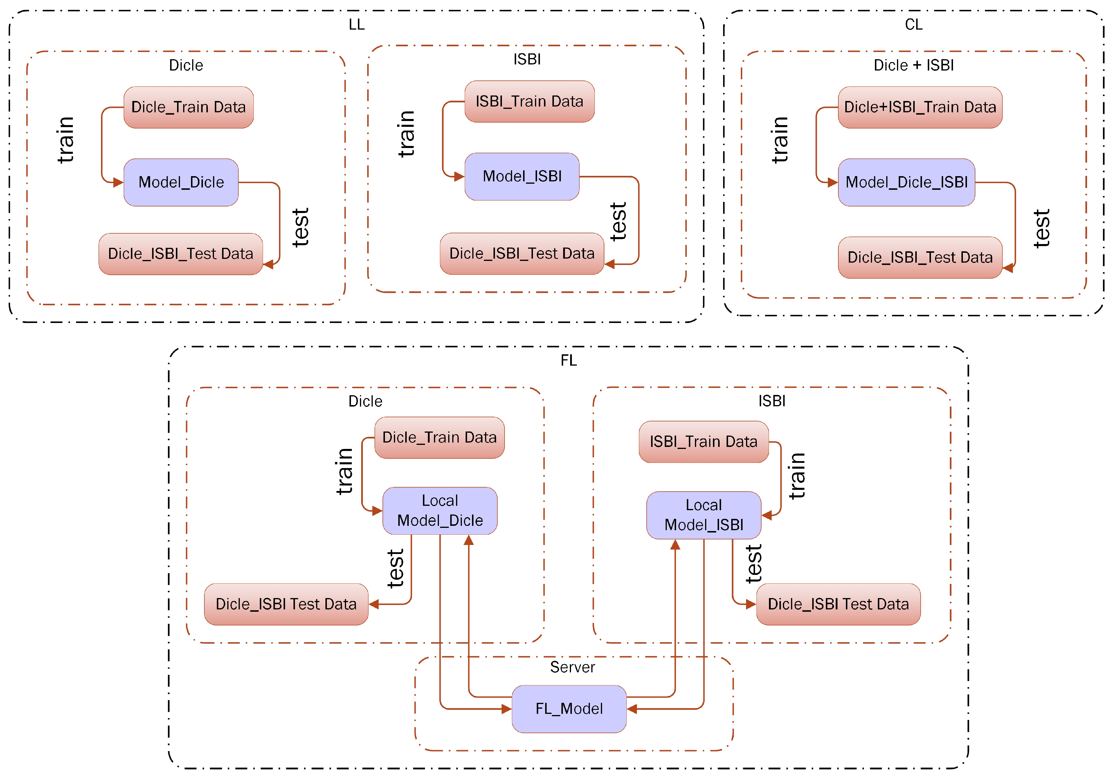
- The impact of FL is thoroughly examined using two distinct dental datasets—the IEEE International Symposium on Biomedical Imaging 2015 Cephalometric X-ray Image Analysis Challenge (ISBI 2015) and Dicle datasets—as a detailed analysis of FL’s contribution is crucial for advancing further clinical applications.
2. Materials and Methods
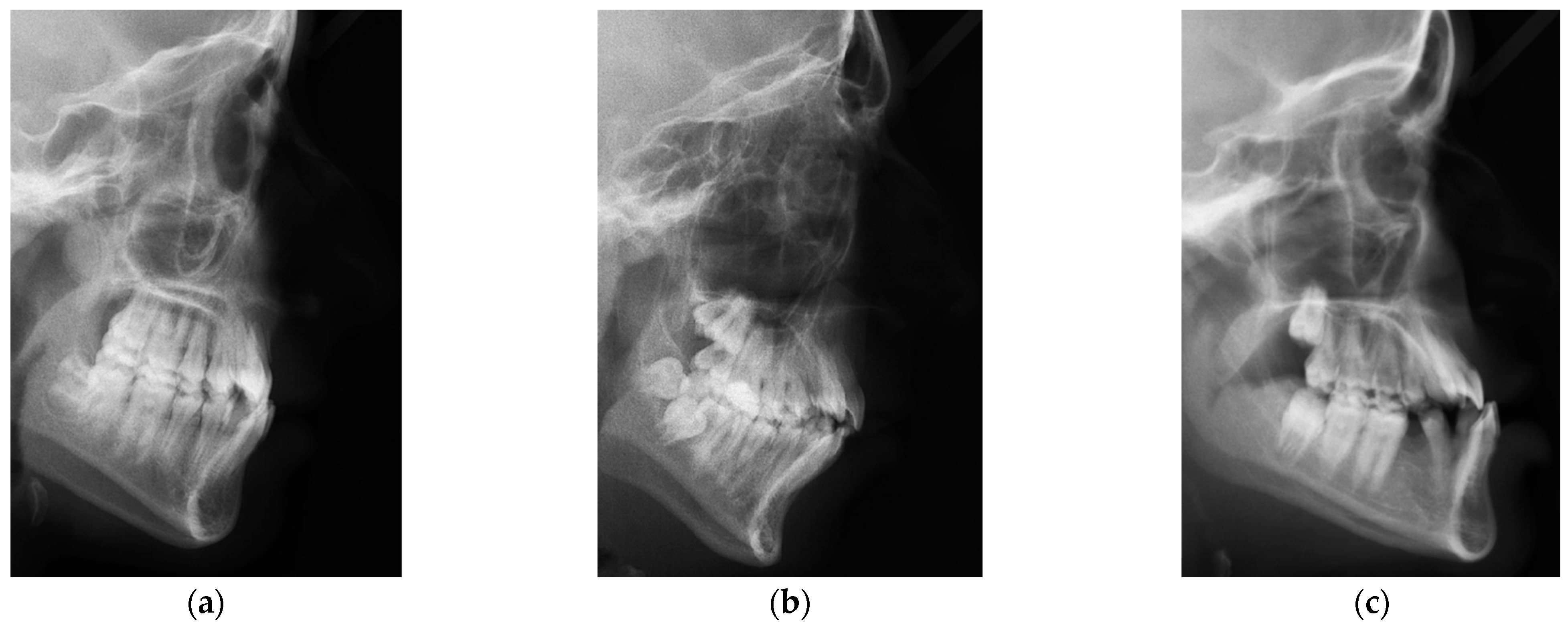
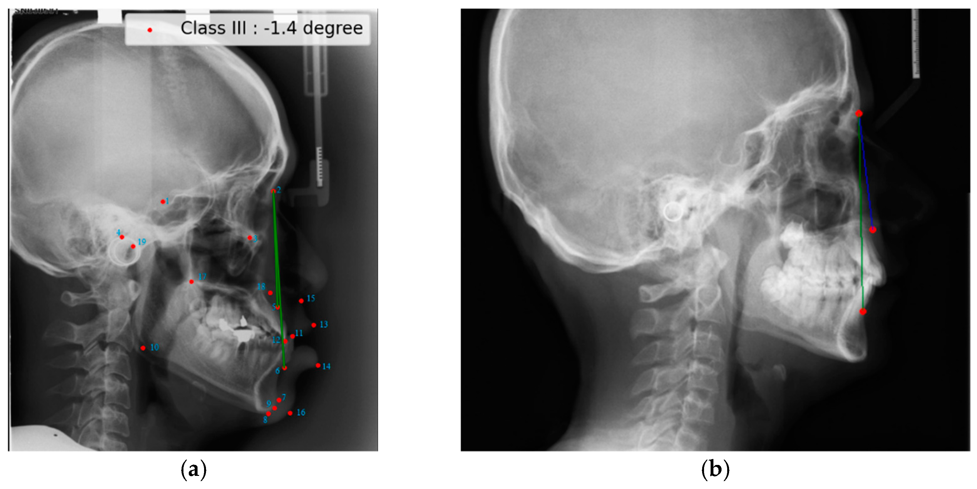
2.1. ISBI Dataset
2.2. Dicle Dataset
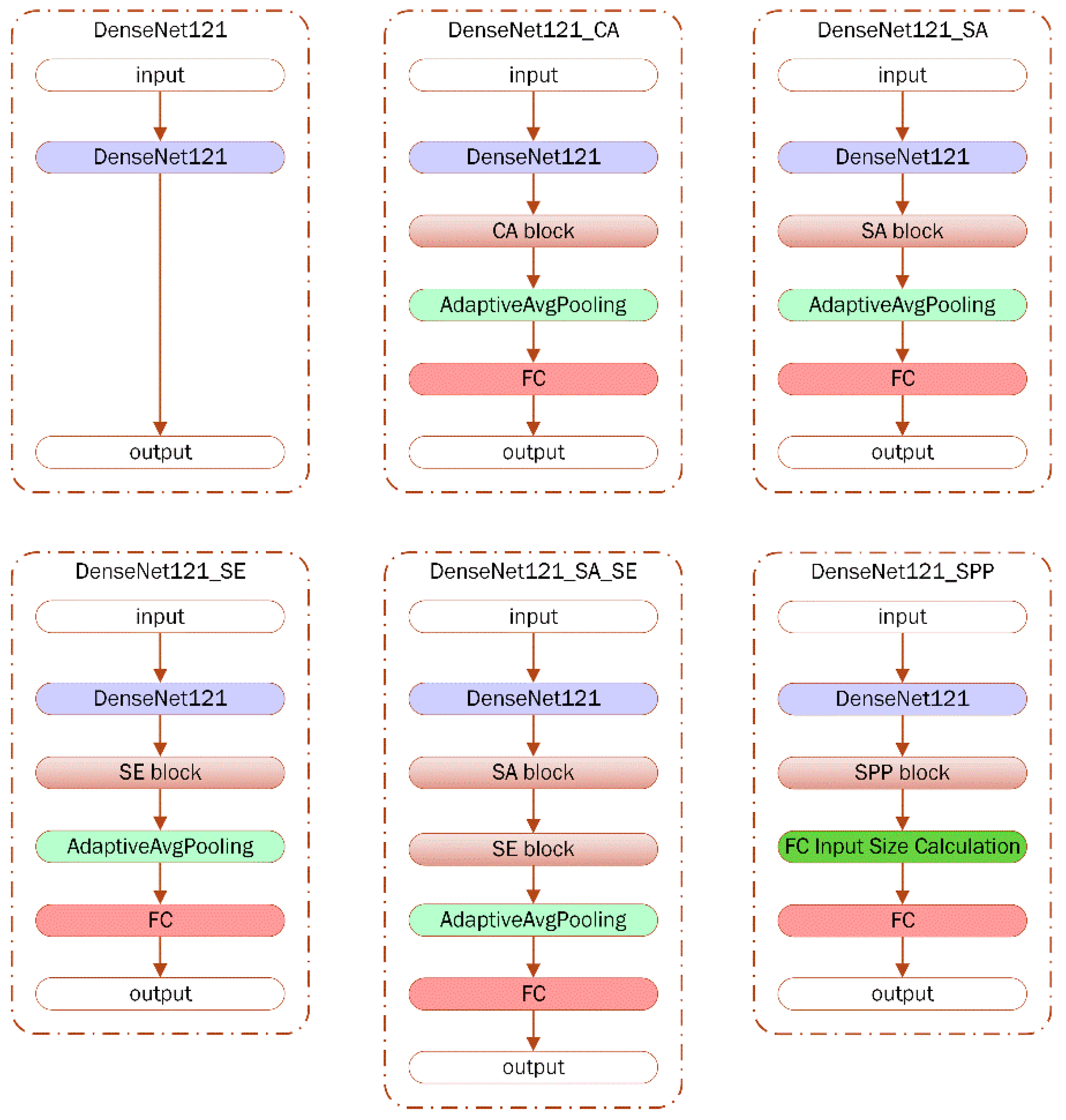
2.3. DenseNet121
2.4. Channel Attention
2.5. Spaital Attention
2.6. Squeeze and Excitation (SE)
2.7. Spatial Pyramid Pooling (SPP)
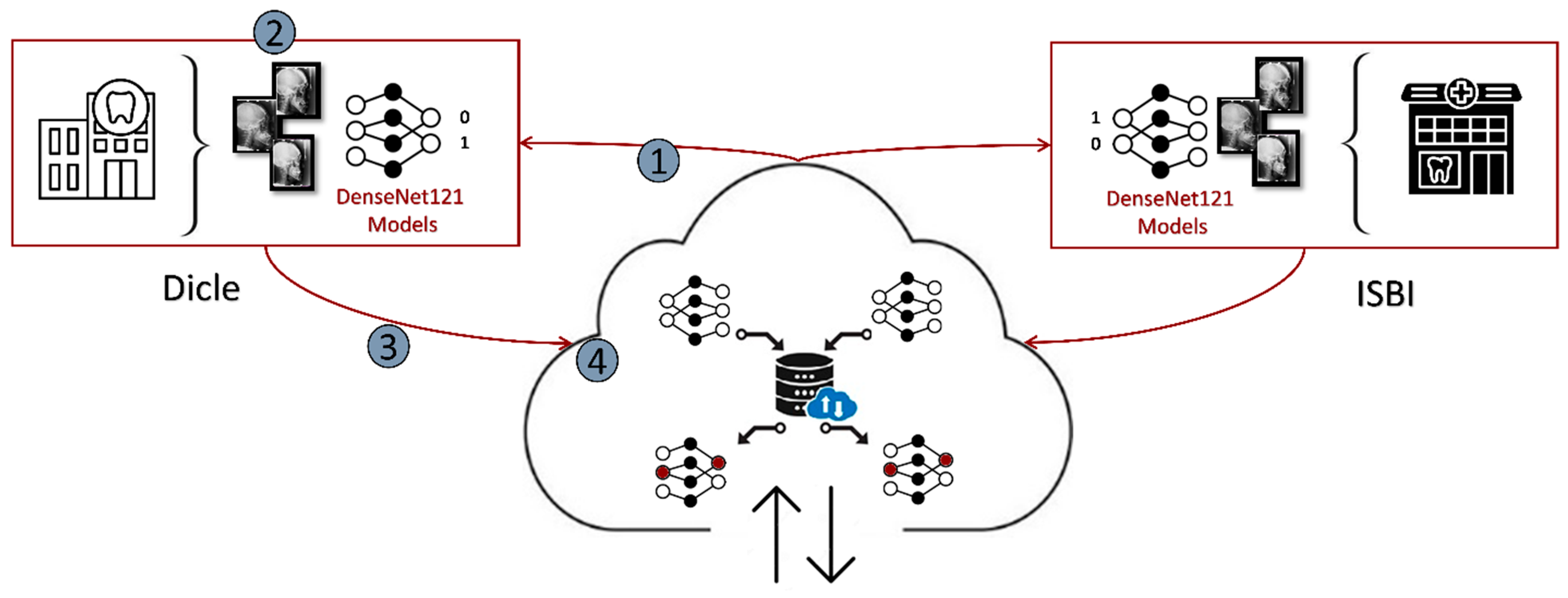
2.8. Setting Federated Learning for Dicle and ISBI Datasets
| Algorithm 1: The Algorithm of the FL setting on the Dicle and ISBI datasets |
| define: 1.a: Clienti, 1 ≤ i ≤ 2 1.b: LocalDataseti // Local Dataset of Clienti 1.c: GlobalModelitr, itr = 0 // The Global DL Model initialized in Server, itr: global iteration number start: do while // 50 global iterations for this study 1.d: Send(GlobalModelitr) // Send the most recent version of the Global DL model at the itrth iteration 2: Train(GlobalModelitr, LocalDataseti) → (GlobalModelitr)i // Each ith client trains the loaded model with its local data for 5 local epochs for this study 3: for each Clienti, do SendServer((GlobalModelitr)i) → (GlobalModelitr)server //The obtained parameter updates of all the locally trained models are sent back to the server 4.a: FaultTolerantFedAvg (GlobalModelitr) → GlobalModelitr //The parameter updates are aggregated on the server and //then a combined Global DL model is obtained for ith iteration 4.b: increment(itr) end |
3. Results
3.1. Selecting the Baseline Model
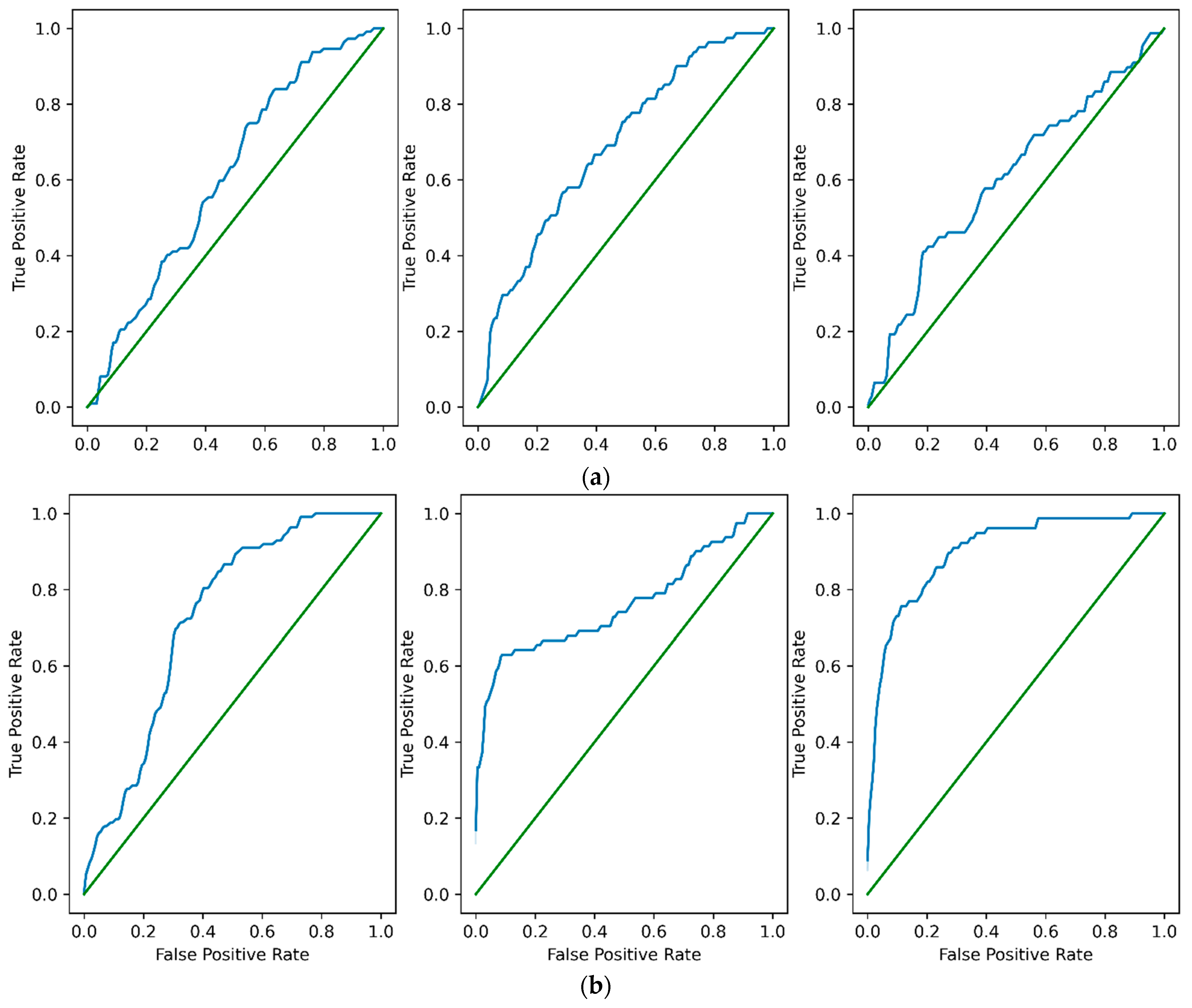
3.2. LL, CL and FL Results
3.3. FL Contribution with Respect to LL and CL
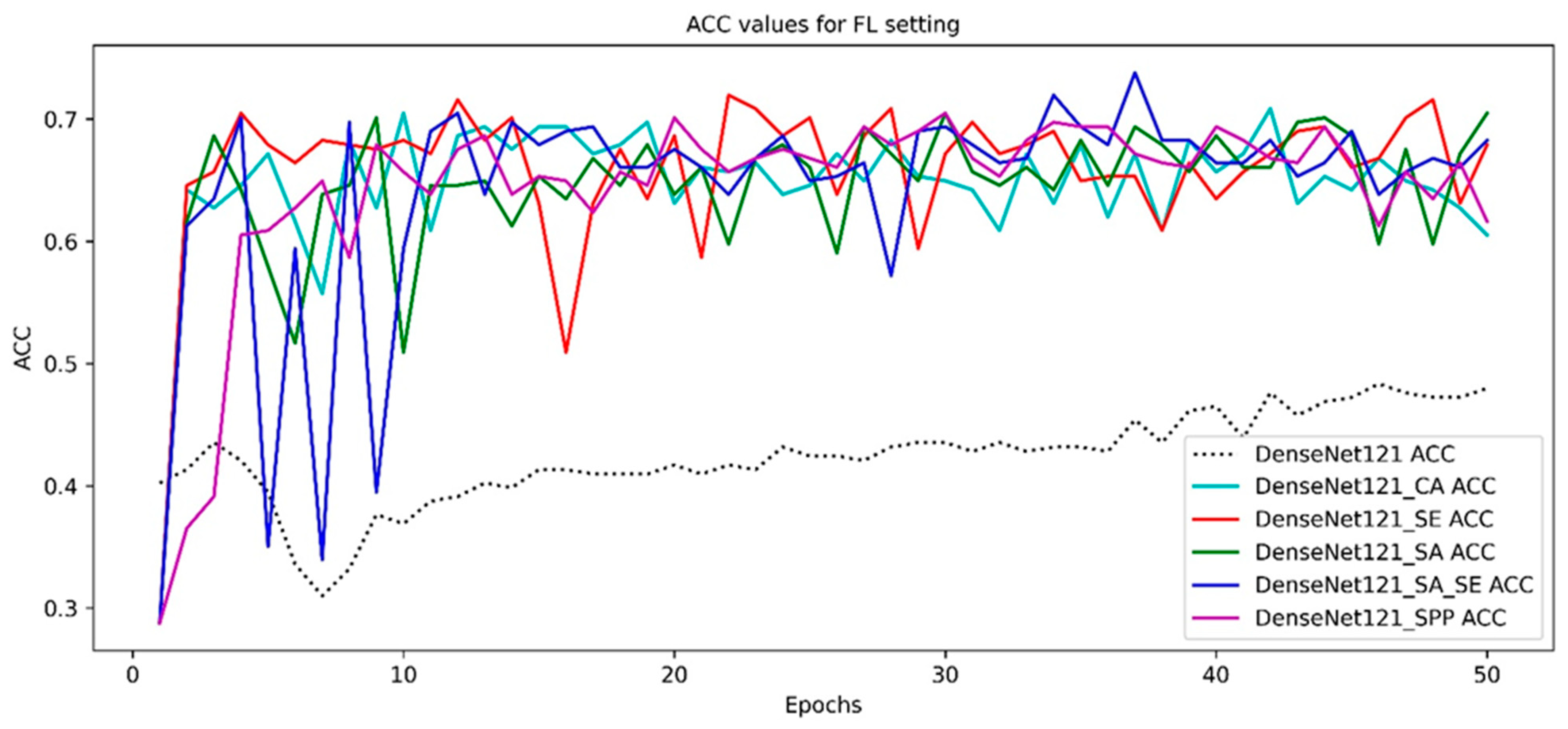
3.4. Model Convergence Analysis in FL Setting
4. Discussion
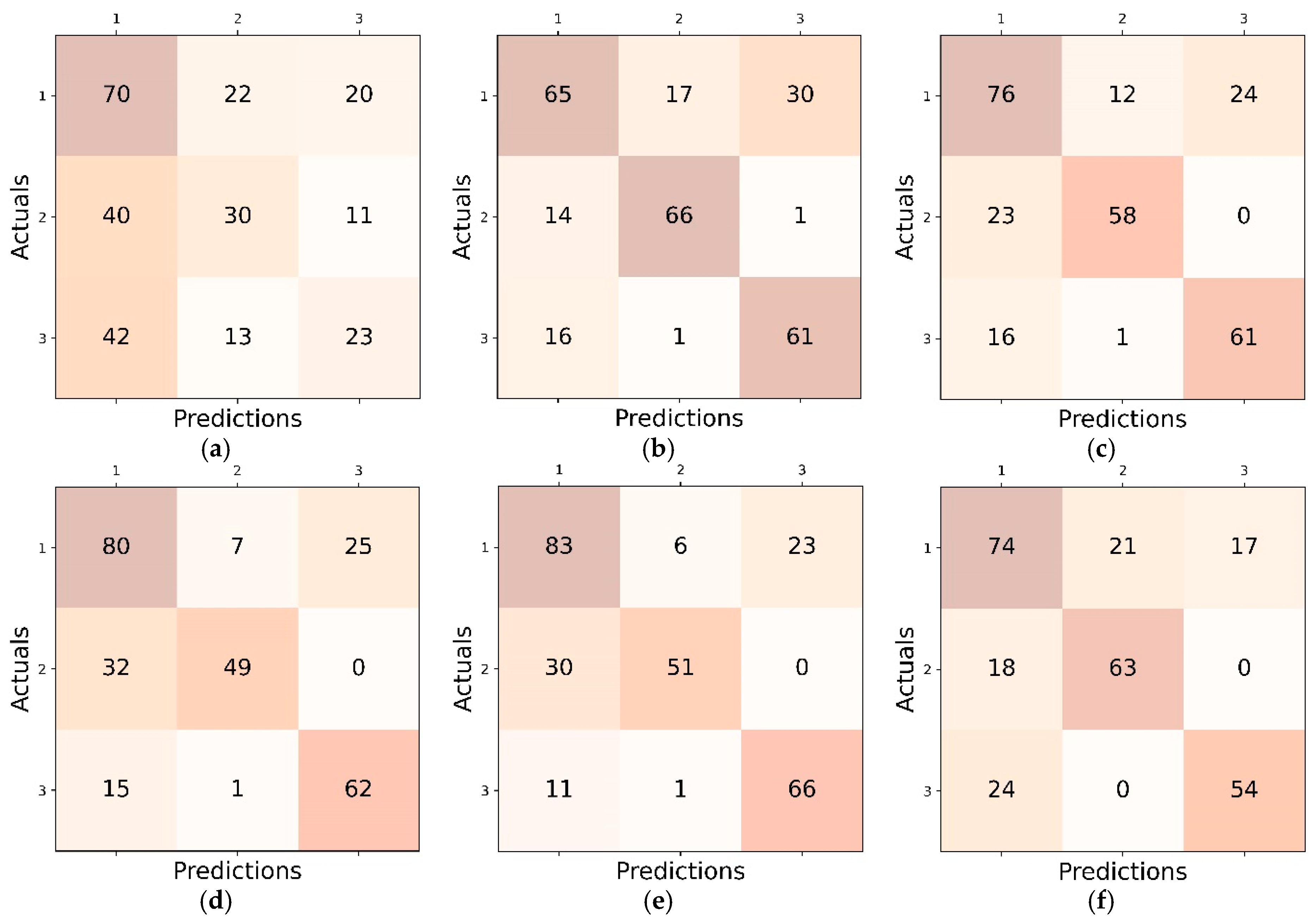
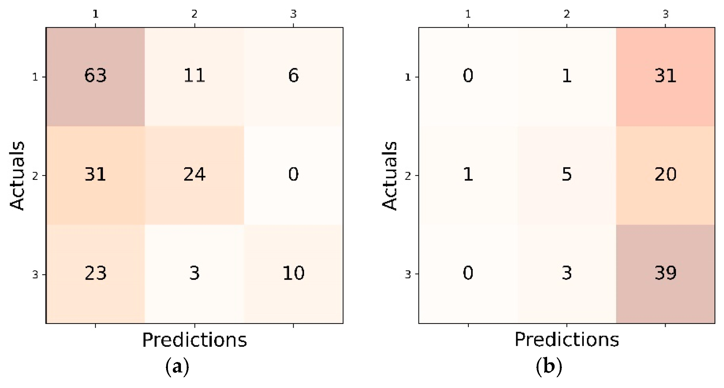
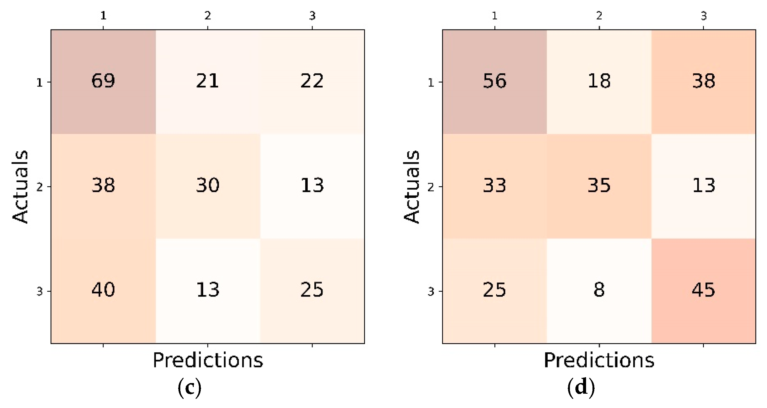
4.1. Inter Class Performance Analysis in LL, CL and FL
4.2. Comparative Analysis with Respect to the Related Works
4.3. Statistical Analysis of FL Contribution
4.4. Evaluating the Labeling Procedures of Dicle and ISBI Datasets
4.5. Limitations and Future Work
5. Conclusions
Author Contributions
Funding
Institutional Review Board Statement
Informed Consent Statement
Data Availability Statement
Acknowledgments
Conflicts of Interest
References
- Wang, C.-W.; Huang, C.-T.; Lee, J.-H.; Li, C.-H.; Chang, S.-W.; Siao, M.-J.; Lai, T.-M.; Ibragimov, B.; Vrtovec, T.; Ronneberger, O.; et al. A benchmark for comparison of dental radiography analysis algorithms. Med. Image Anal. 2016, 31, 63–76. [Google Scholar] [CrossRef] [PubMed]
- Niño-Sandoval, T.C.; Perez, S.V.G.; González, F.A.; Jaque, R.A.; Infante-Contreras, C. An automatic method for skeletal patterns classification using craniomaxillary variables on a Colombian population. Forensic Sci. Int. 2016, 261, 159.e1–159.e6. [Google Scholar] [CrossRef] [PubMed]
- Steiner, C.C. The use of cephalometrics as an aid to planning and assessing orthodontic treatment. Am. J. Orthod. 1960, 46, 721. [Google Scholar] [CrossRef]
- Kim, H.-J.; Kim, K.D.; Kim, D.-H. Deep convolutional neural network-based skeletal classification of cephalometric image compared with automated-tracing software. Sci. Rep. 2022, 12, 11659. [Google Scholar] [CrossRef] [PubMed]
- Rischke, R.; Schneider, L.; Müller, K.; Samek, W.; Schwendicke, F.; Krois, J. Federated Learning in Dentistry: Chances and Challenges. J. Dent. Res. 2022, 101, 1269–1273. [Google Scholar] [CrossRef] [PubMed]
- Liu, J.; Chen, Y.; Li, S.; Zhao, Z.; Wu, Z. Machine learning in orthodontics: Challenges and perspectives. Adv. Clin. Exp. Med. 2021, 30, 1065–1074. [Google Scholar] [CrossRef] [PubMed]
- Schneider, L.; Rischke, R.; Krois, J.; Krasowski, A.; Büttner, M.; Mohammad-Rahimi, H.; Chaurasia, A.; Pereira, N.S.; Lee, J.-H.; Uribe, S.E.; et al. Federated vs Local vs Central Deep Learning of Tooth Segmentation on Panoramic Radiographs. J. Dent. 2023, 135, 104556. [Google Scholar] [CrossRef] [PubMed]
- Liu, S.; Yang, H.H.; Tao, Y.; Feng, Y.; Hao, J.; Liu, Z. Privacy-Preserved Federated Learning for 3D Tooth Segmentation in Intra-Oral Mesh Scans. Front. Commun. Netw. 2022, 3, 907388. [Google Scholar] [CrossRef]
- Lindner, C.; Cootes, T.F. Fully Automatic Cephalometric Evaluation using Random Forest Regression-Voting. In Proceedings of the IEEE International Symposium on Biomedical Imaging (ISBI), Brooklyn, NY, USA, 16–19 April 2015; pp. 1–8. [Google Scholar]
- Kim, Y.-H.; Park, J.-B.; Chang, M.-S.; Ryu, J.-J.; Lim, W.H.; Jung, S.-K. Influence of the Depth of the Convolutional Neural Networks on an Artificial Intelligence Model for Diagnosis of Orthognathic Surgery. J. Pers. Med. 2021, 11, 356. [Google Scholar] [CrossRef] [PubMed]
- Rashmi, S.; Murthy, P.; Ashok, V.; Srinath, S. Cephalometric Skeletal Structure Classification Using Convolutional Neural Networks and Heatmap Regression. SN Comput. Sci. 2022, 3, 336. [Google Scholar] [CrossRef]
- Huang, G.; Liu, Z.; van der Maaten, L.; Weinberger, K.Q. Densely Connected Convolutional Networks Gao. In Proceedings of the IEEE Conference on Computer Vision and Pattern Recognition (CVPR), Honolulu, HI, USA, 21–26 July 2017; pp. 4700–4708. [Google Scholar]
- Ji, Q.; Huang, J.; He, W.; Sun, Y. Optimized Deep Convolutional Neural Networks for Identification of Macular Diseases from Optical Coherence Tomography Images. Algorithms 2019, 12, 51. [Google Scholar] [CrossRef]
- Woo, S.; Park, J.; Lee, J.Y.; Kweon, I.S. CBAM: Convolutional Block Attention Module. In Proceedings of the European Conference on Computer Vision—ECCV 2018, Munich, Germany, 8–14 September 2018; Lecture Notes in Computer Science. Volume 11211, pp. 782–797. [Google Scholar] [CrossRef]
- Hu, J.; Shen, L.; Sun, G. Squeeze-and-Excitation Networks. In Proceedings of the IEEE Conference on Computer Vision and Pattern Recognition (CVPR), Salt Lake City, UT, USA, 18–23 June 2018; pp. 7132–7141. Available online: http://openaccess.thecvf.com/content_cvpr_2018/html/Hu_Squeeze-and-Excitation_Networks_CVPR_2018_paper.html (accessed on 6 January 2025).
- He, K.; Zhang, X.; Ren, S.; Sun, J. Spatial pyramid pooling in deep convolutional networks for visual recognition. In Proceedings of the Computer Vision—ECCV 2014, Zurich, Switzerland, 6–12 September 2014; Lecture Notes in Computer Science (Including Subseries Lecture Notes in Artificial Intelligence and Lecture Notes in Bioinformatics). Volume 8691 LNCS, pp. 346–361. [Google Scholar] [CrossRef]
- McMahan, H.B.; Moore, E.; Ramage, D.; Hampson, S.; Arcas, B.A.Y. Communication-efficient learning of deep networks from decentralized data. In Proceedings of the 20th International Conference on Artificial Intelligence and Statistics, AISTATS 2017, Ft. Lauderdale, FL, USA, 20–22 April 2017; Volume 54. [Google Scholar]
- Nergiz, M. Federated learning-based colorectal cancer classification by convolutional neural networks and general visual representation learning. Int. J. Imaging Syst. Technol. 2023, 33, 951–964. [Google Scholar] [CrossRef]
- Lu, M.Y.; Chen, R.J.; Kong, D.; Lipkova, J.; Singh, R.; Williamson, D.F.; Chen, T.Y.; Mahmood, F. Federated learning for computational pathology on gigapixel whole slide images. Med. Image Anal. 2022, 76, 102298. [Google Scholar] [CrossRef] [PubMed]
- Yang, Q.; Liu, Y.; Chen, T.; Tong, Y. Federated Machine Learning: Concept and applications. ACM Trans. Intell. Syst. Technol. 2019, 10, 1–19. [Google Scholar] [CrossRef]
- Beutel, D.J.; Topal, T.; Mathur, A.; Qiu, X.; Fernandez-Marques, J.; Gao, Y.; Sani, L.; Li, K.H.; Parcollet, T.; de Gusmão, P.P.B.; et al. Flower: A Friendly Federated Learning Research Framework. arXiv 2020, arXiv:2007.14390. [Google Scholar]
- Bonawitz, K.; Ivanov, V.; Kreuter, B.; Marcedone, A.; McMahan, H.B.; Patel, S.; Ramage, D.; Segal, A.; Seth, K. Practical secure aggregation for privacy-preserving machine learning. In Proceedings of the 2017 ACM SIGSAC Conference on Computer and Communications Security, Dallas, TX, USA, 30 October–3 November 2017; pp. 1175–1191. [Google Scholar] [CrossRef]
- Bell, J.H.; Bonawitz, K.A.; Gascón, A.; Lepoint, T.; Raykova, M. Secure Single-Server Aggregation with (Poly)Logarithmic Overhead. In Proceedings of the 2020 ACM SIGSAC Conference on Computer and Communications Security, Virtual Event, USA, 9–13 November 2020; pp. 1253–1269. [Google Scholar] [CrossRef]
- Nan, L.; Tang, M.; Liang, B.; Mo, S.; Kang, N.; Song, S.; Zhang, X.; Zeng, X. Automated Sagittal Skeletal Classification of Children Based on Deep Learning. Diagnostics 2023, 13, 1719. [Google Scholar] [CrossRef] [PubMed]
- Arik, S.Ö.; Ibragimov, B.; Xing, L. Fully automated quantitative cephalometry using convolutional neural networks. J. Med. Imaging 2017, 4, 014501. [Google Scholar] [CrossRef] [PubMed]


| Dicle | ISBI | |||||||
|---|---|---|---|---|---|---|---|---|
| I | II | III | Total | I | II | III | Total | |
| Train | 318 | 226 | 141 | 685 | 48 | 63 | 189 | 300 |
| Test | 80 | 55 | 36 | 171 | 32 | 26 | 42 | 100 |
| Total | 399 | 284 | 180 | 856 | 80 | 89 | 231 | 400 |
| Class Ratio | 0.46 | 0.33 | 0.21 | - | 0.2 | 0.22 | 0.58 | - |
| Dicle | ISBI | |||
|---|---|---|---|---|
| Model | ACC | AUC-ROC | ACC | AUC-ROC |
| DenseNet121 | 0.5400 ± 0.04 | 0.6684 ± 0.04 | 0.6122 ± 0.09 | 0.6293 ± 0.05 |
| VGG_11bn | 0.5179 ± 0.04 | 0.6369 ± 0.03 | 0.5968 ± 0.09 | 0.6414 ± 0.01 |
| ShuffleNet | 0.4623 ± 0.04 | 0.5069 ± 0.03 | 0.5839 ± 0.1 | 0.5219 ± 0.02 |
| InceptionV3 | 0.4960 ± 0.03 | 0.6198 ± 0.04 | 0.6005 ± 0.09 | 0.6025 ± 0.05 |
| AlexNet | 0.5380 ± 0.03 | 0.6655 ± 0.03 | 0.6106 ± 0.1 | 0.6331 ± 0.05 |
| Dicle and ISBI | ||
|---|---|---|
| ACC | AUC-ROC | |
| DenseNet121 | 0.5000 ± 0.01 | 0.6645 ± 0.02 |
| DenseNet121_CA | 0.7333 ± 0.02 | 0.8832 ± 0.01 |
| DenseNet121_SE | 0.7368 ± 0.01 | 0.8840 ± 0.01 |
| DenseNet121_SA | 0.7272 ± 0.02 | 0.8715 ± 0.01 |
| DenseNet121_SA_SE | 0.7345 ± 0.01 | 0.8788 ± 0.01 |
| DenseNet121_SPP | 0.7244 ± 0.01 | 0.8702 ± 0.01 |
| Dicle | ISBI | |||
|---|---|---|---|---|
| ACC | AUC-ROC | ACC | AUC-ROC | |
| DenseNet121 | 0.4347 ± 0.04 | 0.5719 ± 0.07 | 0.3116 ± 0.01 | 0.5345 ± 0.03 |
| DenseNet121_CA | 0.6997 ± 0.01 | 0.8514 ± 0.01 | 0.5802 ± 0.04 | 0.7689 ± 0.03 |
| DenseNet121_SE | 0.6977 ± 0.02 | 0.8548 ± 0.01 | 0.5990 ± 0.04 | 0.7817 ± 0.02 |
| DenseNet121_SA | 0.7076 ± 0.01 | 0.8504 ± 0.01 | 0.5660 ± 0.03 | 0.7627 ± 0.02 |
| DenseNet121_SA_SE | 0.7084 ± 0.01 | 0.8537 ± 0.01 | 0.5935 ± 0.02 | 0.7819 ± 0.02 |
| DenseNet121_SPP | 0.6782 ± 0.01 | 0.8437 ± 0.01 | 0.4901 ± 0.05 | 0.7439 ± 0.01 |
| Dicle and ISBI | ||||||
|---|---|---|---|---|---|---|
| ACC | Precision | Recall | F1 Score | AUC-ROC | Cohen’s Kappa | |
| DenseNet121 | 0.4367 ± 0.03 | 0.4101 ± 0.08 | 0.4045 ± 0.04 | 0.3784 ± 0.08 | 0.5529 ± 0.09 | 0.1061 ± 0.07 |
| DenseNet121_CA | 0.7310 ± 0.01 | 0.7384 ± 0.02 | 0.7310 ± 0.01 | 0.7294 ± 0.01 | 0.8703 ± 0.01 | 0.5935 ± 0.02 |
| DenseNet121_SE | 0.7340 ± 0.01 | 0.7464 ± 0.01 | 0.7340 ± 0.01 | 0.7352 ± 0.01 | 0.8784 ± 0.01 | 0.5964 ± 0.01 |
| DenseNet121_SA | 0.7318 ± 0.02 | 0.7449 ± 0.01 | 0.7318 ± 0.02 | 0.7339 ± 0.02 | 0.8772 ± 0.01 | 0.5931 ± 0.03 |
| DenseNet121_SA_SE | 0.7457 ± 0.01 | 0.7602 ± 0.02 | 0.7457 ± 0.01 | 0.7475 ± 0.01 | 0.8755 ± 0.02 | 0.6139 ± 0.02 |
| DenseNet121_SPP | 0.6987 ± 0.02 | 0.7060 ± 0.02 | 0.6987 ± 0.02 | 0.7006 ± 0.02 | 0.8538 ± 0.01 | 0.5441 ± 0.04 |
| Dicle | ISBI | Dicle and ISBI | |
|---|---|---|---|
| LL vs. FL | LL vs. FL | CL vs. FL | |
| DenseNet121 | 0.002 | 0.1251 | 0.0633 |
| DenseNet121_CA | 0.0313 | 0.1508 | 0.0023 |
| DenseNet121_SE | 0.0363 | 0.1350 | 0.002 |
| DenseNet121_SA | 0.0242 | 0.1658 | −0.0046 |
| DenseNet121_SA_SE | 0.0373 | 0.1522 | −0.0112 |
| DenseNet121_SPP | 0.0205 | 0.2086 | 0.0257 |
| Study | Dataset | Data Size | ACC |
|---|---|---|---|
| Nino-Sandoval et al. [2] | Local | 229 (70% train-val 30% test) | 0.6522 |
| Ibragimov el al. [1] | ISBI | 250 (60% train 40% test) | 0.7664 |
| Lindner and Cootes [1,9] | ISBI | 250 (60% train 40% test) | 0.7583 |
| Arık [25] | ISBI | 250 (60% train 40% test) | 0.7731 |
| Kim et al. [10] | Local | 960 (85% train-val 15% test) | 0.938 |
| Kim et al. [4] | Local | 1574 (92.5% train-val 7.5% test) | 0.96 |
| DenseNet121_SE | Dicle and ISBI | 856 (80% train 20% test) 400 (75% train 25% test) | 0.7368 |
| Dicle | ISBI | Dicle and ISBI | |
|---|---|---|---|
| LL vs. FL | LL vs. FL | CL vs. FL | |
| DenseNet121 | 0.9383 | 0.0001 | 0.009 |
| DenseNet121_CA | 0.0140 | 0.0001 | 0.8698 |
| DenseNet121_SE | 0.0117 | 0.0002 | 0.7542 |
| DenseNet121_SA | 0.0577 | 0.00001 | 0.7530 |
| DenseNet121_SA_SE | 0.0085 | 0.00001 | 0.2871 |
| DenseNet121_SPP | 0.1727 | 0.00006 | 0.0935 |
Disclaimer/Publisher’s Note: The statements, opinions and data contained in all publications are solely those of the individual author(s) and contributor(s) and not of MDPI and/or the editor(s). MDPI and/or the editor(s) disclaim responsibility for any injury to people or property resulting from any ideas, methods, instructions or products referred to in the content. |
© 2025 by the authors. Licensee MDPI, Basel, Switzerland. This article is an open access article distributed under the terms and conditions of the Creative Commons Attribution (CC BY) license (https://creativecommons.org/licenses/by/4.0/).
Share and Cite
Süer Tümen, D.; Nergiz, M. Federated Learning-Based CNN Models for Orthodontic Skeletal Classification and Diagnosis. Diagnostics 2025, 15, 920. https://doi.org/10.3390/diagnostics15070920
Süer Tümen D, Nergiz M. Federated Learning-Based CNN Models for Orthodontic Skeletal Classification and Diagnosis. Diagnostics. 2025; 15(7):920. https://doi.org/10.3390/diagnostics15070920
Chicago/Turabian StyleSüer Tümen, Demet, and Mehmet Nergiz. 2025. "Federated Learning-Based CNN Models for Orthodontic Skeletal Classification and Diagnosis" Diagnostics 15, no. 7: 920. https://doi.org/10.3390/diagnostics15070920
APA StyleSüer Tümen, D., & Nergiz, M. (2025). Federated Learning-Based CNN Models for Orthodontic Skeletal Classification and Diagnosis. Diagnostics, 15(7), 920. https://doi.org/10.3390/diagnostics15070920