
Review of Top-Down Method to Determine Atmospheric Emissions in Port. Case of Study: Port of Veracruz, Mexico

 ,
,  , ,
, , 
Abstract
:1. Introduction
2. Background
2.1. International Maritime Organization and Marine Pollution Regulations for SO2
2.2. SO2 Emission Factor
2.3. Top-Down Method to Determine Atmospheric Emissions
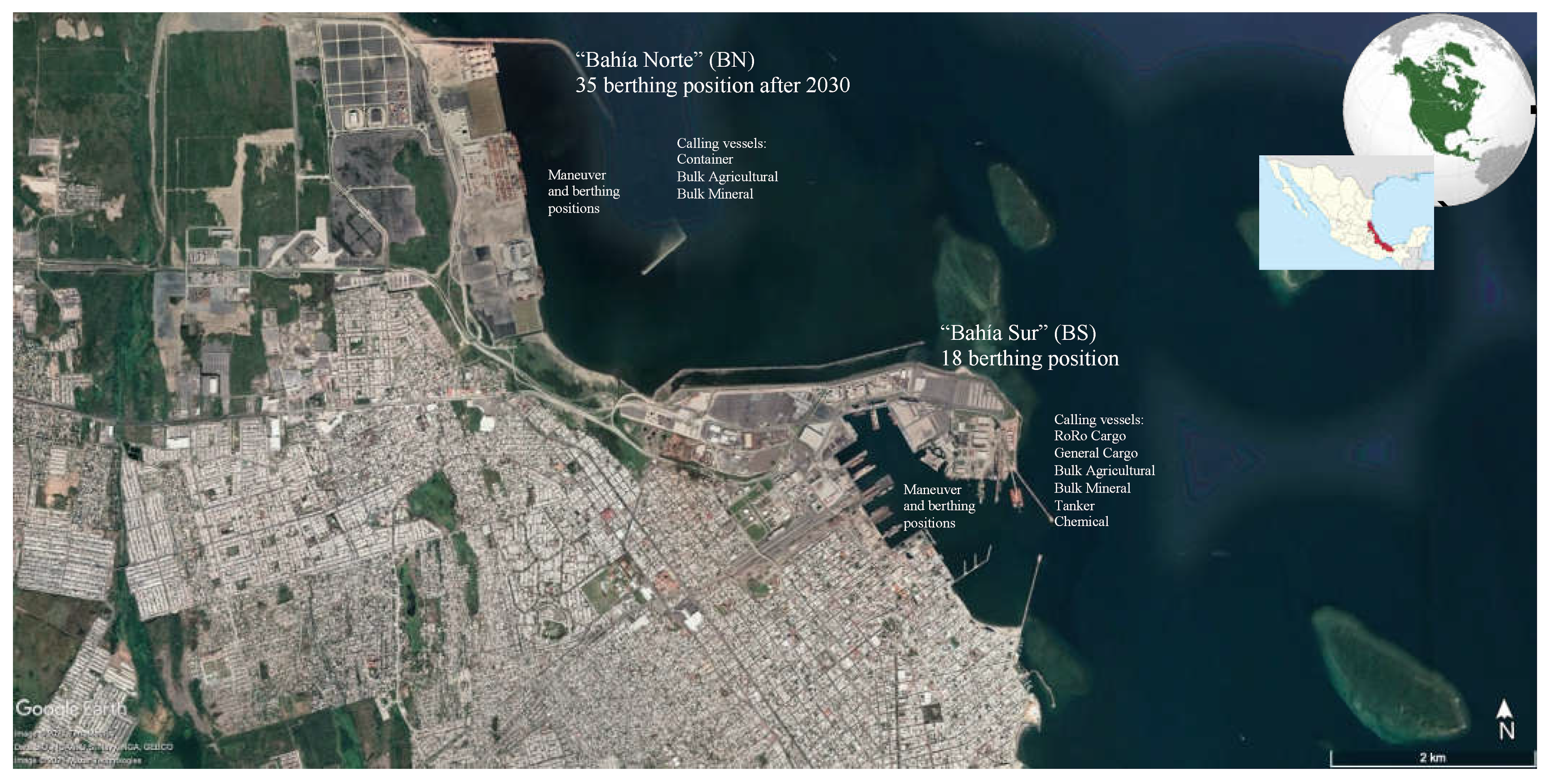
3. Case Study: Port of Veracruz
4. Methodology
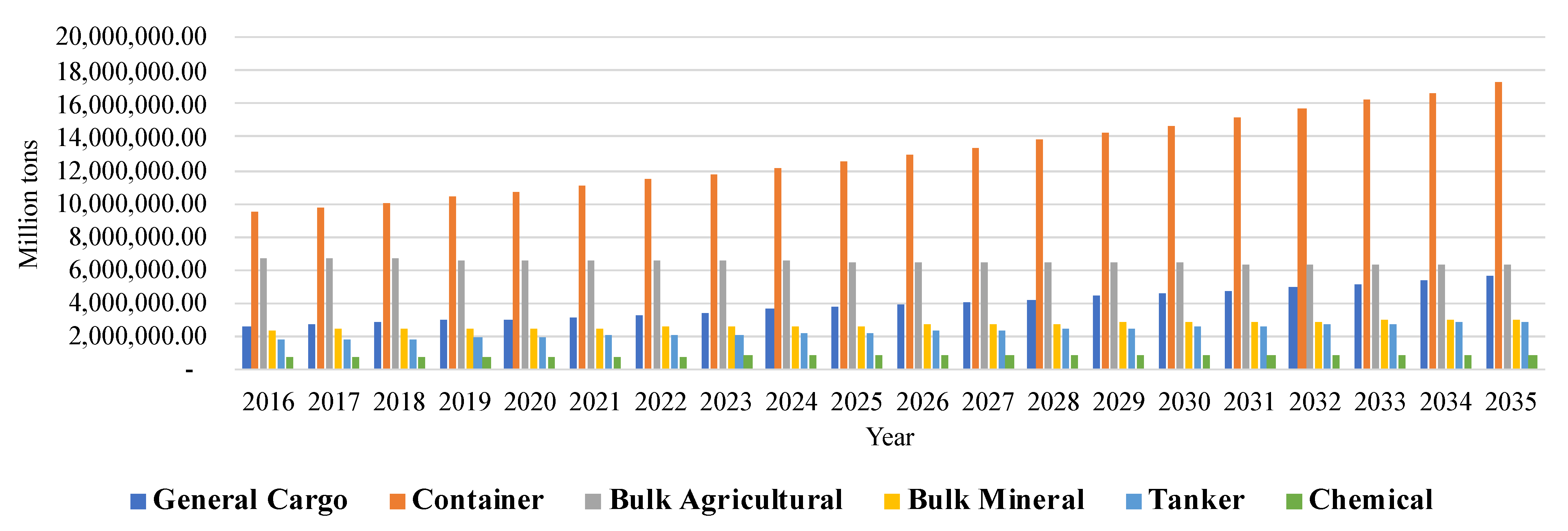
4.1. Database
4.2. Applying to Top-Down Method
- i, j: Berthing and maneuvering position, respectively;
- : Atmospheric Emissions, kgpollutant;
- : Fuel Consumption, , according to vessel type;
- : Emission Factor for SO2, ;
- : Time spent, h, according to vessel type.
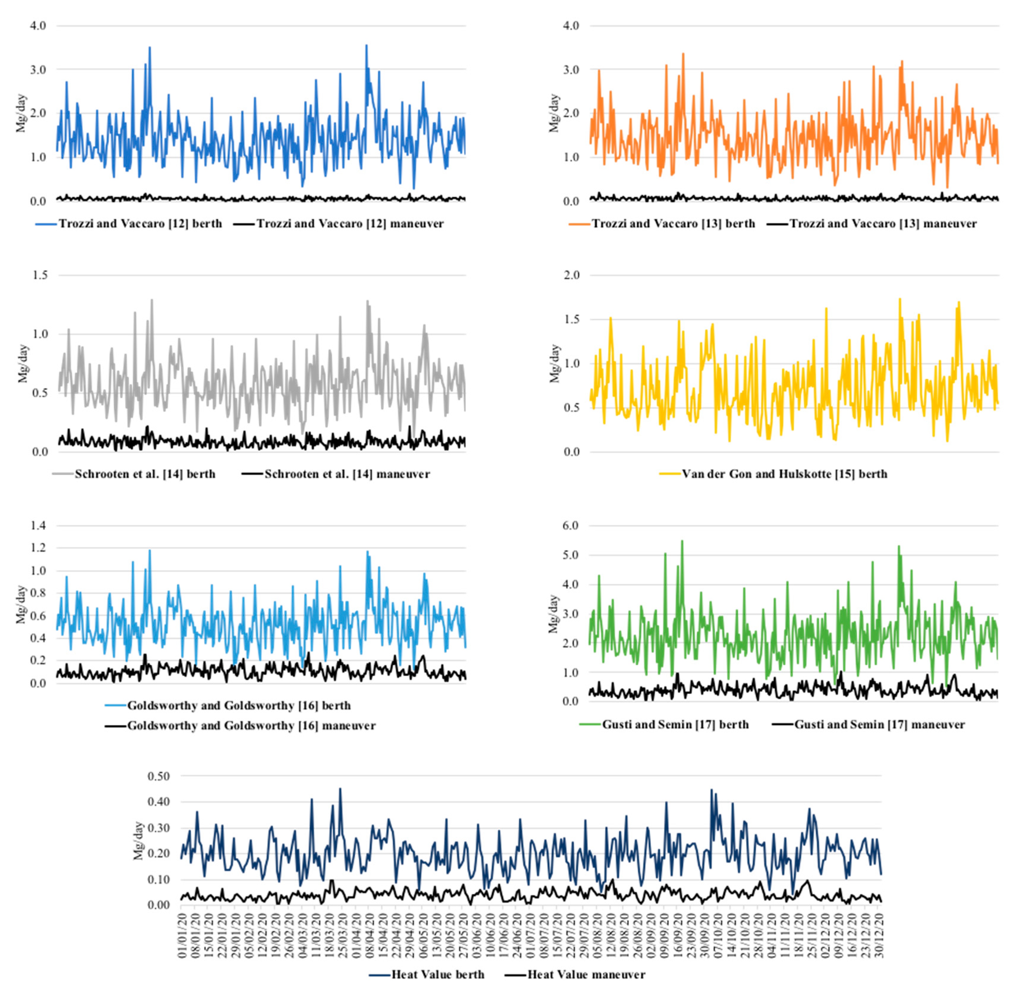
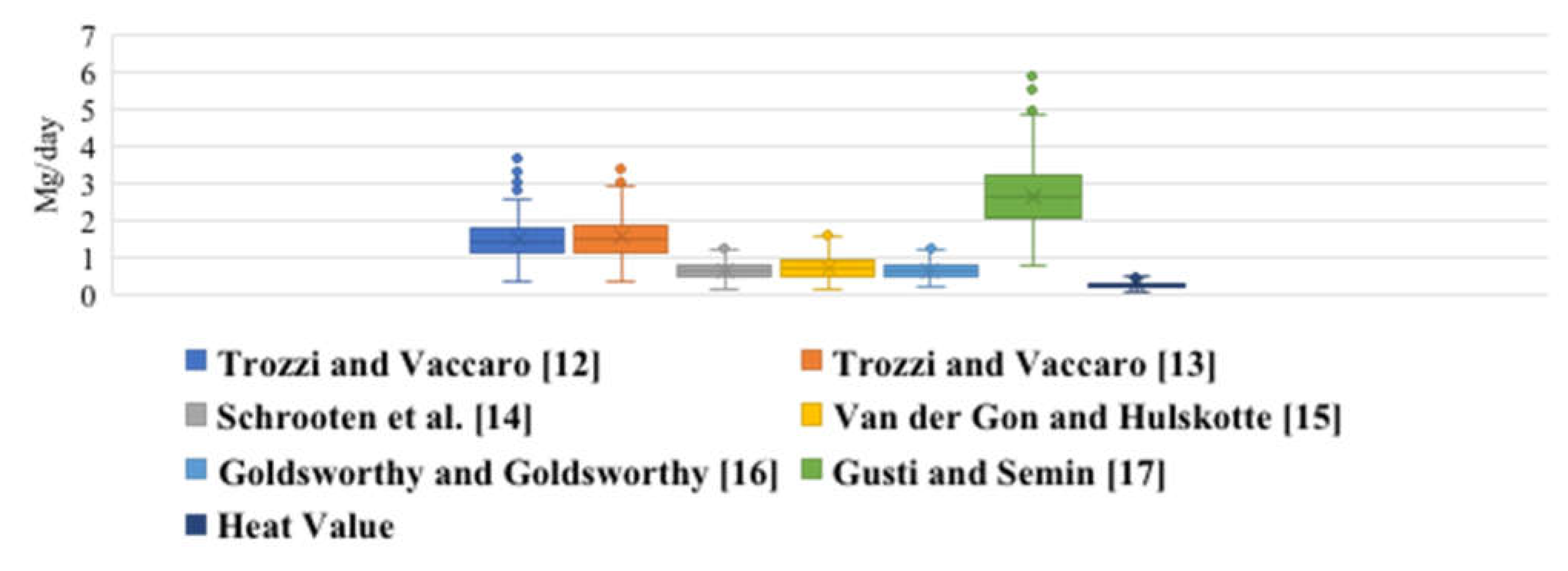
5. Results and Analysis
6. Conclusions
7. Recommendations
8. Future Work
Author Contributions
Funding
Institutional Review Board Statement
Informed Consent Statement
Data Availability Statement
Acknowledgments
Conflicts of Interest
References
- Corbett, J.J.; Koehler, H. Update emissions from ocean shipping. J. Geophys. Res. 2003, 108, 4650. [Google Scholar] [CrossRef]
- USEPA (United States for Environmental Protection Agency). Current Methodologies and Best Practices in Preparing Port Emissions Inventories; Final Report; United States for Environmental Protection Agency: Washington, DC, USA, 2006; pp. 5–44. Available online: https://ntrl.ntis.gov/NTRL/dashboard/searchResults/titleDetail/PB2006112993.xhtml (accessed on 20 February 2021).
- Browing, L.; Bailey, K. Current Methodologies and Best Practices for Preparing Port Emissions Inventories; United States for Environmental Protection Agency: Washington, DC, USA, 2006; pp. 1–20. Available online: http://citeseerx.ist.psu.edu/viewdoc/download?doi=10.1.1.493.5087&rep=rep1&type=pdf (accessed on 15 March 2021).
- Brown, I.; Aldridge, M. Power models and average ship parameter effects on marine emission inventories. J. Air Waste Manag. Assoc. 2019, 69, 752–763. [Google Scholar] [CrossRef] [PubMed]
- USEPA (United States for Environmental Protection Agency). Ports Emissions Inventory Guidance: Methodologies for Estimating Port-Related and Goods Movement Mobile Source Emissions; Final Report; United States for Environmental Protection Agency: Washington, DC, USA, 2020; pp. 5–133. Available online: https://nepis.epa.gov/Exe/ZyPDF.cgi?Dockey=P10102U0.pdf (accessed on 20 February 2021).
- Saputra, H.; Maimun, A.; Koto, J. Estimation and Distribution of Exhaust Ship Emission from Marine Traffic in the Straits of Malacca and Singapore using Automatic Identification System (AIS) Data. J. Mek. 2018, 36, 86–104. Available online: https://jurnalmekanikal.utm.my/index.php/jurnalmekanikal/article/view/58 (accessed on 13 September 2021).
- Song, S. Ship emissions inventory, social cost, and eco-efficiency in Shanghai Yangshan port. Atmos. Environ. 2014, 82, 288–297. [Google Scholar] [CrossRef]
- Knezevic, V.; Radonja, R.; Dundovic, C. Emission Inventory of Marine Traffic for the Port Zadar. Pomorstvo 2018, 32, 239–244. [Google Scholar] [CrossRef] [Green Version]
- Muriel-García, M.; Cerón-Bretón, R.; Cerón-Bretón, J. Air pollution in the Gulf of Mexico. Open J. Ecol. 2016, 6, 32–46. [Google Scholar] [CrossRef] [Green Version]
- Johansson, L.; Jalkanen, J.-P.; Kukkonen, J. Global Assessment of Shipping Emissions in 2015 on a High Spatial and Temporal Resolution. Atmos. Environ. 2017, 167, 403–415. [Google Scholar] [CrossRef]
- Toscano, D.; Murena, F. Atmospheric ship emissions in ports: A review. Correlation with data of ship traffic. Atmos. Environ. X 2019, 4, 100050. [Google Scholar] [CrossRef]
- Trozzi, C.; Vaccaro, R. Air Pollutant Emissions from Ships: High Tyrrhenian Sea Ports Case Study. In Proceedings of the First International Conference PORTS 98 Maritime Engineering and Ports, Genoa, Italy, 28–30 September 1998; pp. 1–11. Available online: https://www.researchgate.net/publication/236857601_Air_pollutant_emissions_from_ships_high_Tyrrhenian_Sea_ports_case_study (accessed on 2 November 2020).
- Trozzi, C.; Vaccaro, R. Methodologies for Estimating Air Pollutants Emissions from Ships: A 2006 Update. In Proceedings of the Environment & Transport 2nd International Scientific Symposium, Reims, France, 12–14 June 2006; pp. 1–8. Available online: https://www.researchgate.net/publication/259470337_Methodologies_for_estimating_air_pollutant_emissions_from_ships_a_2006_update (accessed on 2 November 2020).
- Schrooten, L.; De Vlieger, I.; Panis, L.I.; Styns, K.; Torfs, R. Inventory and forecasting of maritime emissions in the Belgian sea territory, an activity-based emission model. Atmos. Environ. 2008, 42, 667–676. [Google Scholar] [CrossRef]
- Van der Gon, H.D.; Hulskotte, J. Methodologies for Estimating Shipping Emissions in the Netherlands. A Documentation of Currently Used Emission Factors and Related Activity Data; Netherlands Environmental Assessment Agency: AH Bilthoven, The Netherlands, 2010; p. 54. Available online: https://www.pbl.nl/en/publications/methodologies-for-estimating-shipping-emissions-in-the-netherlands (accessed on 20 December 2020).
- Goldsworthy, L.; Goldsworthy, B. Modelling of ship engine exhaust emissions in ports and extensive coastal waters based on terrestrial AIS—An Australian case study. Environ. Model. Softw. 2015, 63, 45–60. [Google Scholar] [CrossRef]
- Gusti, A.P.; Semin, S. The Effect of Vessel Speed on Fuel Consumption and Exhaust Gas Emissions. Am. J. Appl. Sci. 2016, 9, 1046–1053. [Google Scholar] [CrossRef] [Green Version]
- Zamora, V.E. Prevención Del Deterioro Significativo Por Bióxido de Azufre Por La Operación Del Recinto Portuario de Veracruz. Master’s Thesis, Universidad Nacional Autónoma de México, Mexico City, Mexico, 2019. Available online: http://132.248.9.195/ptd2019/enero/0784057/Index.html (accessed on 15 October 2021).
- Antonio, D.R.E. Evaluación Del Impacto Potencial En La Calidad Del Aire Por Partículas Debido a La Operación Del Recinto Portuario de Veracruz. Master’s Thesis, Universidad Nacional Autónoma de México, Mexico City, Mexico, 2019. Available online: http://132.248.9.195/ptd2019/noviembre/0797593/Index.html (accessed on 15 October 2021).
- Fuentes, G.G.; Baldasano, R.J.M.; Sosa, E.R.; Granados, H.E.; Zamora, V.E.; Antonio, D.R.E.; Kahl, W.J.D. Estimation of atmospheric emissions from maritime activity in the Veracruz port, Mexico. J. Air Waste Manag. Assoc. 2021, 71, 934–948. [Google Scholar] [CrossRef]
- Fuentes, G.G.; Echeverría, R.S.; Recio, J.M.B.; Kahl, J.D.W.; Hernández, E.G.; Jímenez, A.L.A.; Durán, R.E.A. Atmospheric Emissions in Ports Due to Maritime Traffic in Mexico. J. Mar. Sci. Eng. 2021, 9, 1186. [Google Scholar] [CrossRef]
- Fuentes, G.G.; Bravo, A.H.; Sosa, E.R.; Rosas, A.S.; Magaña, R.V.; Caetano, D.E.; Vázquez, C.G. Spatial and temporal variability of atmospheric mercury concentrations emitted from a coal-fired power plant in Mexico. J. Air Waste Manag. Assoc. 2017, 67, 973–985. [Google Scholar] [CrossRef]
- Jagangiri, S.; Nikolova, N.; Tenekedjiev, K. Application of a Developed Dispersion Model to Port of Brisbane. Am. J. Environ. Sci. 2018, 14, 156–169. [Google Scholar] [CrossRef]
- Murena, F.; Mocerino, L.; Quaranta, F.; Toscano, D. Impact on air quality of cruise ship emissions in Naples, Italy. Atmos. Environ. 2018, 187, 70–83. [Google Scholar] [CrossRef]
- Bai, S.; Wen, Y.; He, L.; Liu, Y.; Zhang, Y.; Yu, Q.; Ma, W. Single-Vessel Plume Dispersion Simulation: Method and a Case Study Using CALPUFF in the Yantian Port Area, Shenzhen (China). Int. J. Environ. Res. Public Health 2020, 17, 7831. [Google Scholar] [CrossRef]
- Mocerino, L.; Murena, F.; Quaranta, F.; Toscano, D. A methodology for the design of an effective air quality monitoring network in port areas. Sci. Rep. 2020, 10, 300. [Google Scholar] [CrossRef] [Green Version]
- Pan, K.; Lim, M.Q.; Kraft, M.; Mastorakos, E. Development of a moving point source model fro shipping emission dispersion modelling in EPISODE-CityChem v1.3. Geosci. Model Dev. 2021, 14, 4509–4534. [Google Scholar] [CrossRef]
- IMO (International Maritime Organization). Cutting Sulphur Oxide Emissions. Available online: https://www.imo.org/en/MediaCentre/HotTopics/Pages/Sulphur-2020.aspx (accessed on 31 March 2021).
- UNCTAD (United Nations Conference on Trade and Development). Review of Maritime Transport; United Nation Publications: Geneva, Switzerland, 2020; p. 133. Available online: https://unctad.org/webflyer/review-maritime-transport-2020 (accessed on 25 February 2021).
- Viana, M.; Hammingh, P.; Colette, A.; Querol, X.; Degraeuwe, B.; De Vlieger, I.; Van Aardenne, J. Impact of maritime transport emissions on coastal air quality in Europe. Atmos. Environ. 2014, 90, 96–105. [Google Scholar] [CrossRef]
- Prati, M.; Costagliola, M.; Quaranta, F.; Murena, F. Assessment of air quality in the port of Naples. J. Air Waste Manag. Assoc. 2015, 65, 970–979. [Google Scholar] [CrossRef] [PubMed] [Green Version]
- Xiao, Q.; Li, M.; Liu, H.; Fu, M.; Deng, F.; Lv, Z.; Man, H.; Jin, X.; Liu, S.; He, K. Characteristics of marine shipping emissions at berth: Profiles for particulate matter and volatile organic compounds. Atmos. Chem. Phys. 2018, 18, 9527–9545. [Google Scholar] [CrossRef] [Green Version]
- Wang, X.; Shen, Y.; Pan, J.; Zhang, Y.; Louie, P.; Li, M.; Fu, Q. Atmospheric pollution from ships and its impact on local air quality at a port site in Shanghai. Atmos. Chem. Phys. 2019, 19, 6315–6330. [Google Scholar] [CrossRef] [Green Version]
- Corbett, J.; Winebrake, J.; Green, E.; Kasibhatla, P.; Eyring, V.; Lauer, A. Mortality from Ship Emissions: A Global Assessment. Environ. Sci. Technol. 2007, 41, 8512–8518. [Google Scholar] [CrossRef]
- Muller, D.; Uibel, S.; Takemura, M.; Klingelhoefer, D.; Groneberg, D. Ships, ports and particulate air pollution—An analysis of recent studies. J. Occup. Med. Toxicol. 2011, 6, 31. Available online: http://www.occup-med.com/content/6/1/31 (accessed on 20 October 2021). [CrossRef] [Green Version]
- Sofiev, M.; Winebrake, J.; Johansson, L.; Carr, E.; Prank, M.; Soares, J.; Vira, J.; Kouznetsov, R.; Jalkanen, J.-P.; Corbett, J. Cleaner fuels for ships provide public health benefits with climate tradeoffs. Nat. Commun. 2018, 9, 406. [Google Scholar] [CrossRef] [Green Version]
- Mwase, N.; Ekstrom, A.; Jonson, J.; Svensson, E.; Jalkanen, J.-P.; Wichmann, J.; Molnár, P.; Stockfelt, L. Health Impact of Air Pollution from Shipping in the Baltic Sea: Effects of Different Spatial Resolution in Sweden. Int. J. Environ. Res. Public Health 2020, 17, 7963. [Google Scholar] [CrossRef]
- ENTEC (European Commission). Directorate General Environment. Service Contract on Ship Emissions: Quantification of Ship Emissions; Final Report; ENTEC UK Limited: Newcastle Upon Tyne, UK, 2002; p. 48. Available online: https://ec.europa.eu/environment/air/pdf/chapter2_ship_emissions.pdf (accessed on 31 January 2020).
- Cooper, D.; Gustafsson, T. Methodology for calculating emissions from ships: 1. In Update of Emission Factors; Swedish Methodology for Environmental Data; SMED; Swedish Meteorological and Hydrological Institute: Norrkoping, Sweden, 2004; pp. 13–28. Available online: https://www.diva-portal.org/smash/get/diva2:1117198/FULLTEXT01.pdf (accessed on 27 March 2020).
- USEPA (United States for Environmental Protection Agency). Chapter 2: Ocean Going Vessels. In Current Methodologies in Preparing Mobile Source Port-Related Emission Inventories; Final Report; United States for Environmental Protection Agency: Washington, DC, USA, 2009; pp. 1–26. Available online: https://www.epa.gov/sites/production/files/2016-06/documents/2009-port-inventory-guidance.pdf (accessed on 28 December 2020).
- ENTEC (European Commission). Directorate General Environment. Service Contract on Ship Emissions Inventory; Final Report; ENTEC UK Limited: Newcastle, UK, 2010; pp. 1–66. Available online: https://uk-air.defra.gov.uk/assets/documents/reports/cat15/1012131459_21897_Final_Report_291110.pdf (accessed on 28 December 2020).
- EMEP/EEA (European Monitoring and Evaluation Programme/European Environment Agency). Navigation (Shipping); EMEP/EEA: Copenhagen, Denmark, 2019; pp. 1–40. Available online: https://www.eea.europa.eu/publications/emep-eea-guidebook-2019/part-b-sectoral-guidance-chapters/1-energy/1-a-combustion/1-a-3-d-navigation/view (accessed on 10 January 2020).
- Jalkanen, J.P.; Brink, A.; Kalli, J.; Pettersson, H.; Kukkonen, J.; Stipa, T. A modelling system for the exhaust emissions of marine traffic and its application in the Baltic Sea area. Atmos. Chem. Phys. Discuss. 2009, 9, 9209–9223. [Google Scholar] [CrossRef] [Green Version]
- Jalkanen, J.P.; Johansson, L.; Kukkonen, J.; Brink, A.; Kalli, J.; Stipa, T. Extension of an assessment model of ship traffic exhaust emissions for particulate matter and carbon monoxide. Atmos. Chem. Phys. 2012, 12, 2641–2659. [Google Scholar] [CrossRef] [Green Version]
- Jalkanen, J.P.; Johansson, L.; Kukkonen, J. A comprehensive inventory of the ship traffic exhaust emissions in the Baltic Sea from 2006 to 2009. Ambio 2014, 43, 311–324. [Google Scholar] [CrossRef] [Green Version]
- Trozzi, C. Emission Estimate Methodology for Maritime Navigation. In Proceedings of the 19th International Emissions Inventory Conference, USEPA, San Antonio, TX, USA, 20–30 September 2010; pp. 1–11. Available online: https://www.researchgate.net/publication/233387511_Emission_estimate_methodology_for_maritime_navigation (accessed on 20 June 2021).
- Gutiérrez, M.J.; Durán-Granados, V.; Uriondo, Z.; Ángel-Llamas, J. Emission-factor uncertainties in maritime transport in the Strait of Gibraltar, Spain. Atmos. Meas. Tech. Discuss. 2012, 5, 5953–5991. [Google Scholar] [CrossRef]
- Moreno-Gutiérrez, J.; Calderay, F.; Saborido, N.; Boile, M.; Valero, R.; Durán-Grados, V. Methodologies for estimating shipping emissions and energy consumption: A comparative analysis of current methods. Energy 2015, 86, 603–616. [Google Scholar] [CrossRef]
- USEPA (United States for Environmental Protection Agency). U. S.—Mexico Cooperation on Reducing Emissions from Ships through a Mexican Emission Control Area: Development of the First National Mexican Emission Inventories for Ships Using the Waterway Network Ship Traffic, Energy, and Environmental Model (STEEM); United States for Environmental Protection Agency: Washington, DC, USA, 2015; p. 13. Available online: https://www.epa.gov/sites/production/files/2015-07/documents/steem-report-final-s508.pdf (accessed on 25 April 2021).
- Bialystocki, N.; Konovessis, D. On the estimation of ship’s fuel consumption and speed curve: A statistical approach. J. Ocean Eng. Sci. 2016, 1, 157–166. [Google Scholar] [CrossRef] [Green Version]
- Simonsen, M.; Walnum, H.J.; Gossling, S. Model for Estimation of Fuel Consumption of Cruise Ships. Energies 2018, 11, 1059. [Google Scholar] [CrossRef] [Green Version]
- PMDP. Programa Maestro de Desarrollo Portuario del Puerto de Veracruz, 2016-2021; Secretaría de Comunicaciones y Transportes: Ciudad de Veracruz, México, 2021; p. 65. Available online: https://www.puertodeveracruz.com.mx/wordpress/quienes-somos/programa-maestro-de-desarrollo-portuario-2016-2021/ (accessed on 20 February 2021).
- APIVER (Administración Portuaria Integral de Veracruz). Resumen Mensual; APIVER: Ciudad de Veracruz, México, 2020. Available online: https://www.puertodeveracruz.com.mx/wordpress/estadisticas-2/resumen/ (accessed on 31 March 2021).
- UNCTAD (United Nations Conference on Trade and Development). Maritime Profile in Mexico; United Nation Publications: Geneva, Switzerland, 2021; Available online: https://unctadstat.unctad.org/CountryProfile/MaritimeProfile/en-GB/484/index.html (accessed on 25 February 2021).
- Baldasano, J.M.; Güereca, P.; López, E.; Gassó, S.; PJimenez-Guerrero. Development of a high-resolution (1km × 1km, 1h) emission model for Spain: The High Elective Resolution Modelling Emission System (HERMES). Atmos. Environ. 2008, 42, 7215–7233. [Google Scholar] [CrossRef]


| Type of Vessel | Ships | GT Average | Tonnage Average/Ship | Stay at Port Average/Ship, h | ||||
|---|---|---|---|---|---|---|---|---|
| 2019 | 2020 | 2019 | 2020 | 2019 | 2020 | 2019 | 2020 | |
| General Cargo | 358 | 296 | 28,979 | 30,672 | 5020 | 4487 | 87.6 | 74.7 |
| RoRo Cargo | 230 | 178 | 57,407 | 57,329 | 6800 | 6766 | 44.6 | 42.0 |
| Container No Specialized | 168 | 110 | 27,031 | 22,486 | 7509 | 6240 | 20.5 | 16.1 |
| Container Specialized | 494 | 532 | 60,435 | 59,153 | 20,031 | 16,887 | 21.1 | 17.1 |
| Bulk Agricultural | 236 | 223 | 24,589 | 25,284 | 31,482 | 31,138 | 154.6 | 158.4 |
| Bulk Mineral | 125 | 148 | 20,314 | 19,182 | 19,255 | 19,275 | 92.4 | 93.8 |
| Tanker | 208 | 188 | 28,367 | 26,839 | 12,708 | 12,489 | 88.3 | 94.0 |
| Chemical | 177 | 186 | 13,807 | 14,479 | 7206 | 9958 | 54.3 | 60.7 |
| 1996 | 1861 | 32,616.13 | 31,928.00 | 13,751.38 | 13,405.00 | 70.4 | 69.6 | |
| Method | FC by Type of Ship | GT | SFC | Power of ME (PME) and AE (PAE) | LF | Time Spent in Berthing Position | Emission Factor |
|---|---|---|---|---|---|---|---|
| Trozzi and Vaccaro [12] | Table 3 | Yes | - | - | - | Yes | Yes |
| Trozzi and Vaccaro [13] | Table 4 | Yes | - | - | - | Yes | Yes |
| Schrooten et al. [14] | Table 5 | Yes | Yes | Yes | Yes | Yes | Yes |
| Goldsworthy and Goldsworthy [16] | Yes | Yes | Yes | Yes | Yes | Yes | |
| Gusti and Semin [17] | Yes | Yes | Yes | - | Yes | Yes | |
| Van der Gon and Hulskotte [15] | Table 6 | Yes | - | - | - | Yes | Yes |
| Considering Heat Value for MDO | Table 7 | Yes | Yes | Yes | Yes | Yes | Yes |
| Type of Vessel | Adjustment of the FC | |
|---|---|---|
| General Cargo | Berthing: 0.2 Maneuvering: 0.4 | |
| RoRo Cargo | ||
| Container | ||
| Bulk Agricultural | ||
| Bulk Mineral | ||
| Tanker | ||
| Chemical |
| Type of Vessel | Adjustment of the FC | |
|---|---|---|
| General Cargo | Berthing: 0.2 Maneuvering: 0.4 | |
| RoRo Cargo | ||
| Container | ||
| Bulk Agricultural | ||
| Bulk Mineral | ||
| Tanker | ||
| Chemical |
| Type of Vessel | Schrooten et al. [14] To Obtain Divided by | |||||
| Goldsworthy and Goldsworthy [16] Gusti and Semin [17]: To Obtain Divided by | ||||||
| SFC at berth [38] | LF [38] | PME, kW [46] | Average Gross Tonne, [53] | Average Vessel Ratio [46] | PAE, kW | |
| General Cargo | 225 | 0.2 | 30,672 | 0.23 | 2745 | |
| RoRo Cargo | 227 | 0.2 | 57,329 | 0.24 | 4640 | |
| Container | 223 | 0.2 | 40,820 | 0.25 | 7639 | |
| Bulk Agricultural | 222 | 0.2 | 22,233 | 0.30 | 2118 | |
| Bulk Mineral | ||||||
| Tanker | 222 | 0.4 | 20,659 | 0.30 | 1867 | |
| Chemical | ||||||
| Type of Vessel | |
|---|---|
| General Cargo | 5.4 |
| RoRo Cargo | 6.9 |
| Container | 5.0 |
| Bulk Agricultural | 2.4 |
| Bulk Mineral | |
| Tanker | 19.3 |
| Chemical |
| Type of Vessel | ||||||
| Consumption | LF [38] | PME, kW [46] | Average GT, [53] | Average Vessel Ratio [46] | PAE, kW | |
| General Cargo | 0.2 | 30,672 | 0.23 | 2745 | ||
| RoRo Cargo | 0.2 | 57,329 | 0.24 | 4640 | ||
| Container | 0.2 | 40,820 | 0.25 | 7639 | ||
| Bulk Agricultural | 0.2 | 22,233 | 0.30 | 2118 | ||
| Bulk Mineral | ||||||
| Tanker | 0.4 | 20,659 | 0.30 | 1867 | ||
| Chemical | ||||||
| Type of Vessel | Time Spent in Berthing Position Average/Vessel, h [53] | Time Spent in Maneuver Position Average/Vessel, h [53] |
|---|---|---|
| General Cargo | 74.7 | 1.0 |
| RoRo Cargo | 42.0 | 1.0 |
| Container | 16.6 | 1.0 |
| Bulk Agricultural | 158.4 | 1.0 |
| Bulk Mineral | 93.8 | 1.0 |
| Tanker | 94.0 | 1.0 |
| Chemical | 60.7 | 1.0 |
| Method | Trozzi and Vaccaro [12] | Trozzi and Vaccaro [13] | Schrooten et al. [14] | Van der Gon and Hulskotte [15] | Goldsworthy and Goldsworthy [16] | Gusti and Semin [17] | Heat Value |
|---|---|---|---|---|---|---|---|
| Trozzi and Vaccaro [12] | 1.00000 | 0.93027 | 0.90468 | 0.55793 | 0.86807 | 0.92246 | 0.86493 |
| Trozzi and Vaccaro [13] | 0.93027 | 1.00000 | 0.89452 | 0.49810 | 0.86388 | 0.91322 | 0.86230 |
| Schrooten et al. [14] | 0.90468 | 0.89452 | 1.00000 | 0.67816 | 0.97557 | 0.92957 | 0.97518 |
| Van der Gon and Hulskotte [15] | 0.55793 | 0.49810 | 0.67816 | 1.00000 | 0.65994 | 0.47072 | 0.65812 |
| Goldsworthy and Goldsworthy [16] | 0.86807 | 0.86388 | 0.97557 | 0.65994 | 1.00000 | 0.94481 | 0.99995 |
| Gusti and Semin [17] | 0.92246 | 0.91322 | 0.92957 | 0.47072 | 0.94481 | 1.00000 | 0.94399 |
| Heat Value | 0.86493 | 0.86230 | 0.97518 | 0.65812 | 0.99995 | 0.94399 | 1.00000 |
Publisher’s Note: MDPI stays neutral with regard to jurisdictional claims in published maps and institutional affiliations. |
© 2022 by the authors. Licensee MDPI, Basel, Switzerland. This article is an open access article distributed under the terms and conditions of the Creative Commons Attribution (CC BY) license (https://creativecommons.org/licenses/by/4.0/).
Share and Cite
Fuentes García, G.; Sosa Echeverría, R.; Baldasano Recio, J.M.; W. Kahl, J.D.; Antonio Durán, R.E. Review of Top-Down Method to Determine Atmospheric Emissions in Port. Case of Study: Port of Veracruz, Mexico. J. Mar. Sci. Eng. 2022, 10, 96. https://doi.org/10.3390/jmse10010096
Fuentes García G, Sosa Echeverría R, Baldasano Recio JM, W. Kahl JD, Antonio Durán RE. Review of Top-Down Method to Determine Atmospheric Emissions in Port. Case of Study: Port of Veracruz, Mexico. Journal of Marine Science and Engineering. 2022; 10(1):96. https://doi.org/10.3390/jmse10010096
Chicago/Turabian StyleFuentes García, Gilberto, Rodolfo Sosa Echeverría, José María Baldasano Recio, Jonathan D. W. Kahl, and Rafael Esteban Antonio Durán. 2022. "Review of Top-Down Method to Determine Atmospheric Emissions in Port. Case of Study: Port of Veracruz, Mexico" Journal of Marine Science and Engineering 10, no. 1: 96. https://doi.org/10.3390/jmse10010096
APA StyleFuentes García, G., Sosa Echeverría, R., Baldasano Recio, J. M., W. Kahl, J. D., & Antonio Durán, R. E. (2022). Review of Top-Down Method to Determine Atmospheric Emissions in Port. Case of Study: Port of Veracruz, Mexico. Journal of Marine Science and Engineering, 10(1), 96. https://doi.org/10.3390/jmse10010096