
Real-Time Validation of a Novel IAOA Technique-Based Offset Hysteresis Band Current Controller for Grid-Tied Photovoltaic System

 , ,
, ,  , , ,
, , ,
Abstract
:1. Introduction
- Design of a novel IAOA optimization technique for a microgrid-connected PV system.
- Application of conventional and offset hysteresis band current controller in a PV-based microgrid.
- Realization of enhanced performance with an IAOA-based offset hysteresis band current controller.
- Establishment of the effectiveness of the proposed control algorithm in mitigating harmonics from the grid current.
- Comparative analysis of novel metaheuristic algorithm-based conventional and offset hysteresis band current controllers with MATLAB/Simulink and OPAL-RT simulator with linear and nonlinear loads.
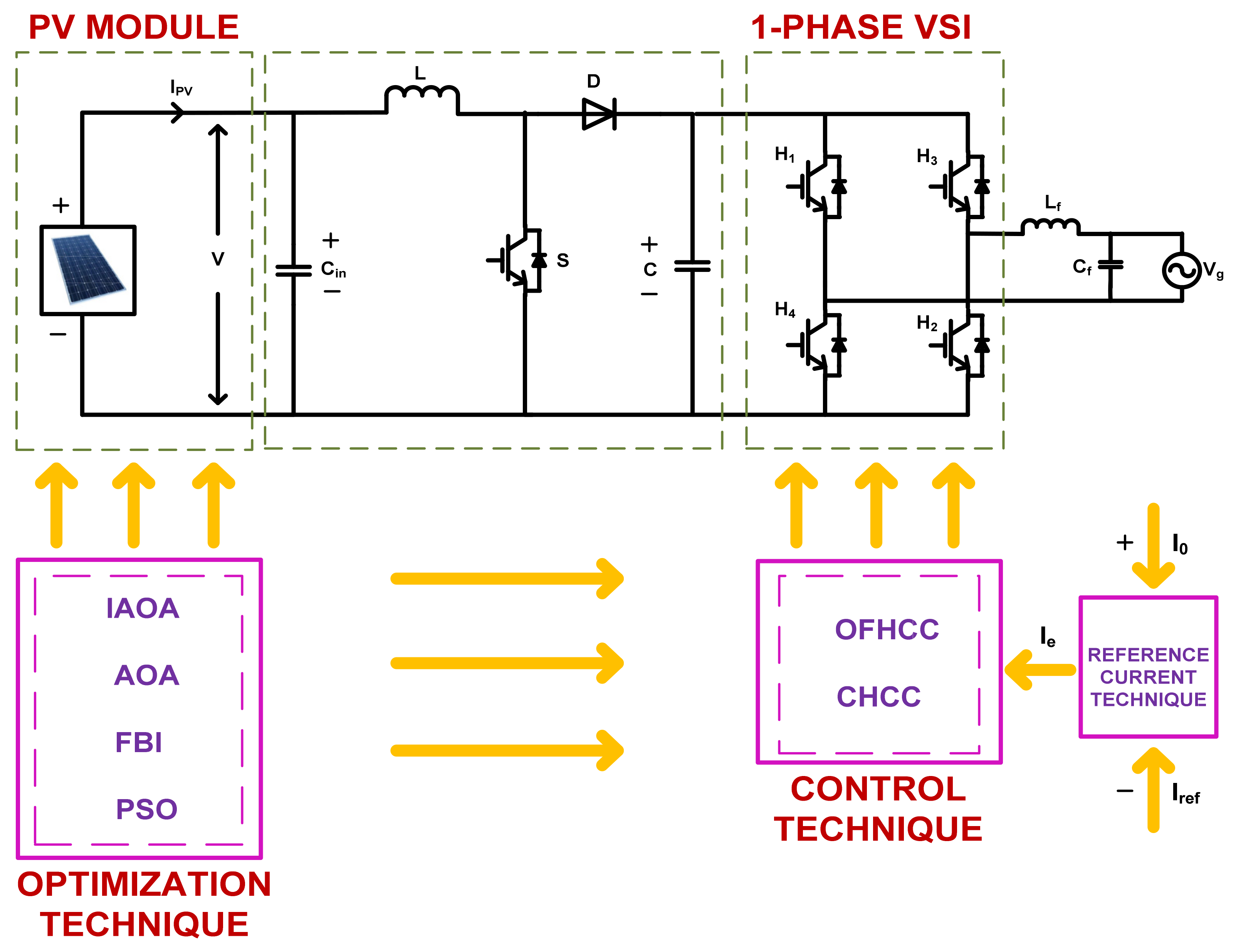
2. System Modelling
2.1. PV Module Model
2.2. Modeling of Single-Phase PWM-VSI
2.3. Proposed Methodology
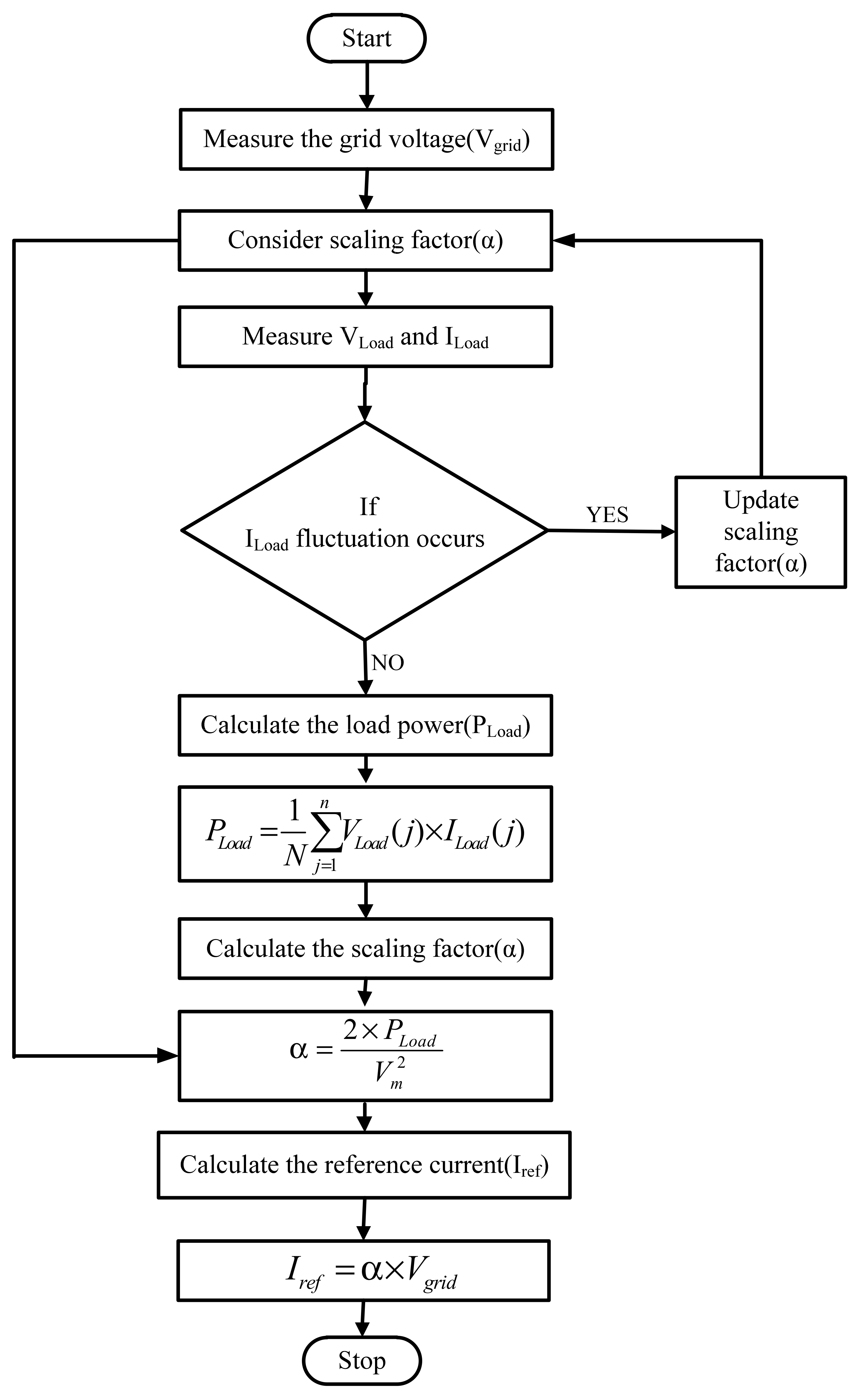
2.4. Reference Current Technique
3. Analysis of Advanced Controllers
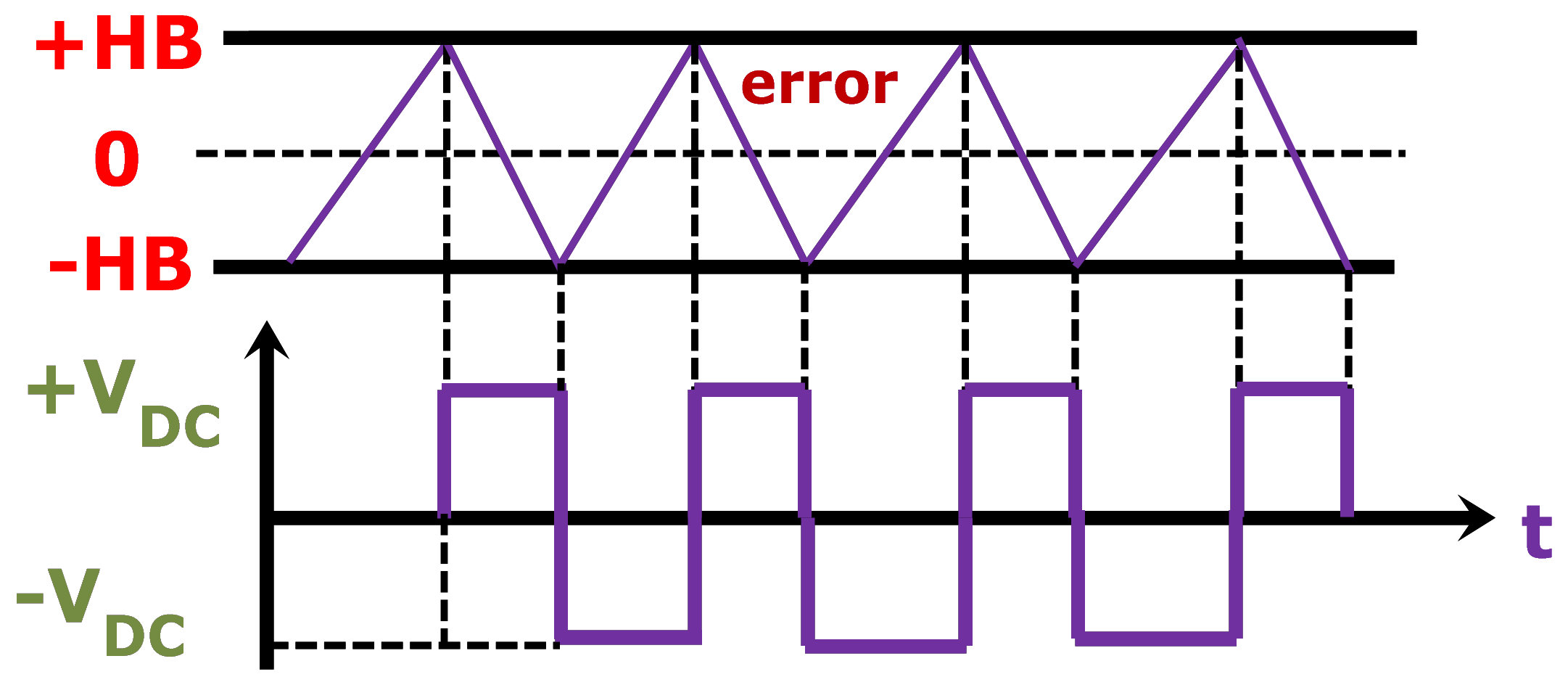
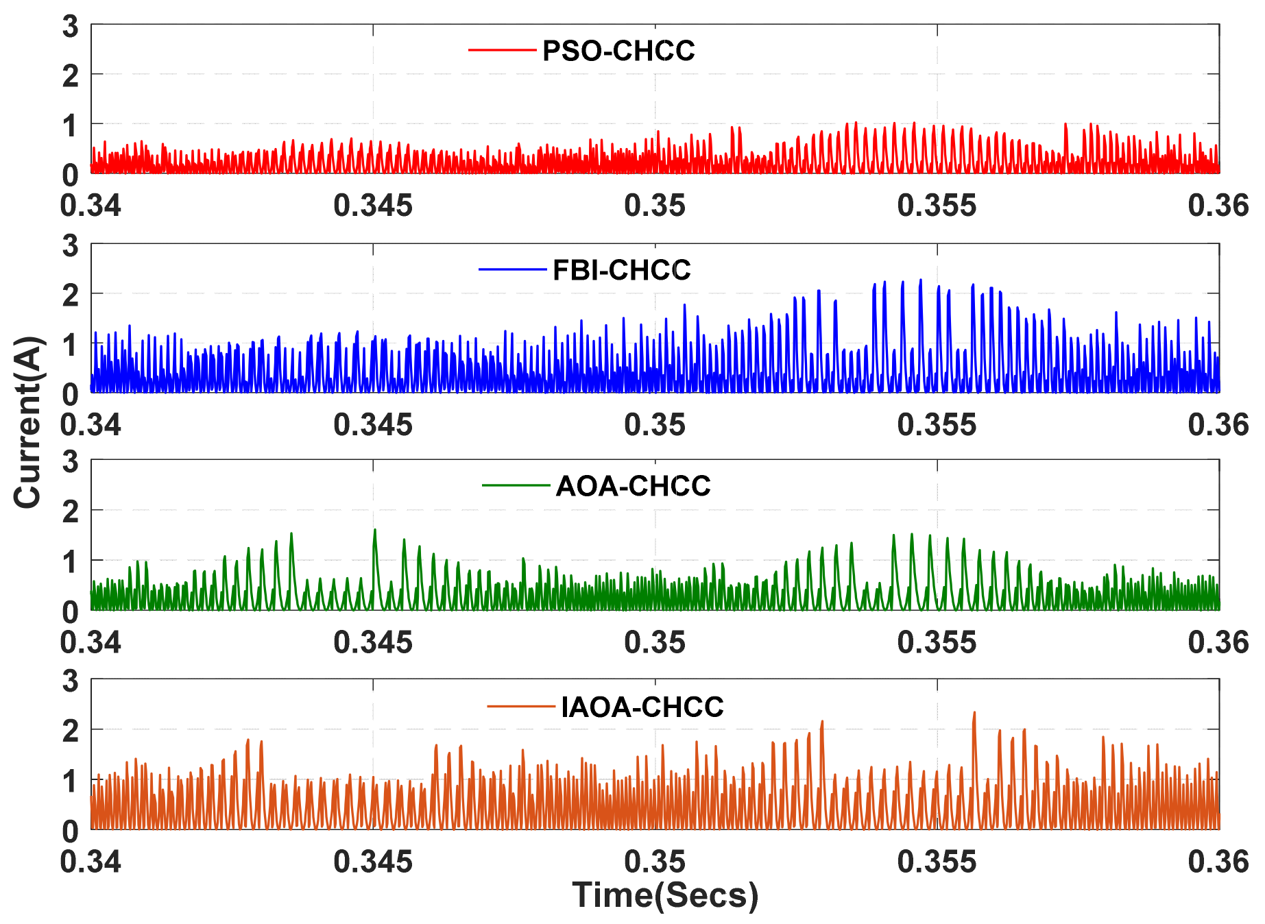
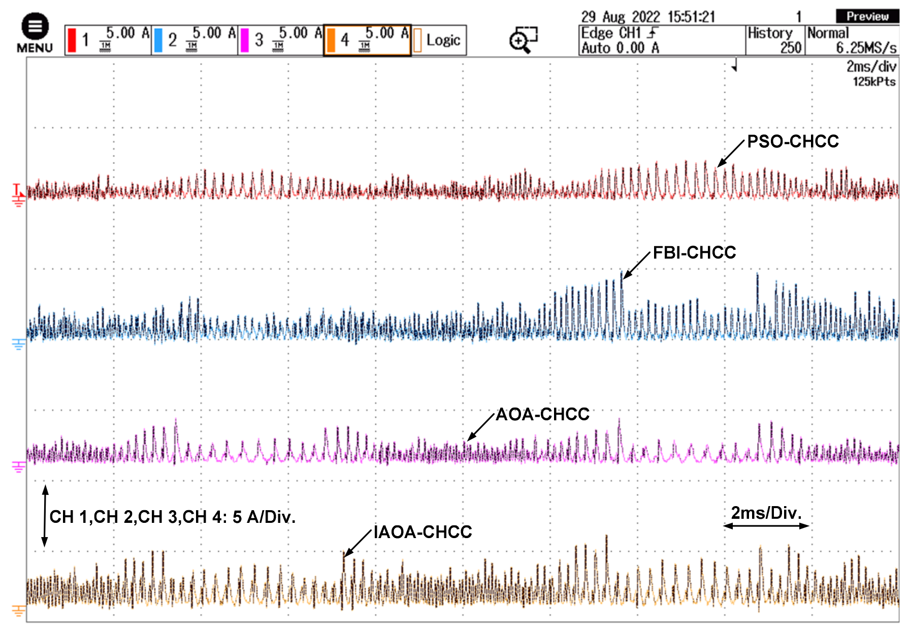
3.1. Conventional Hysteresis Band Current Controller (CHCC)
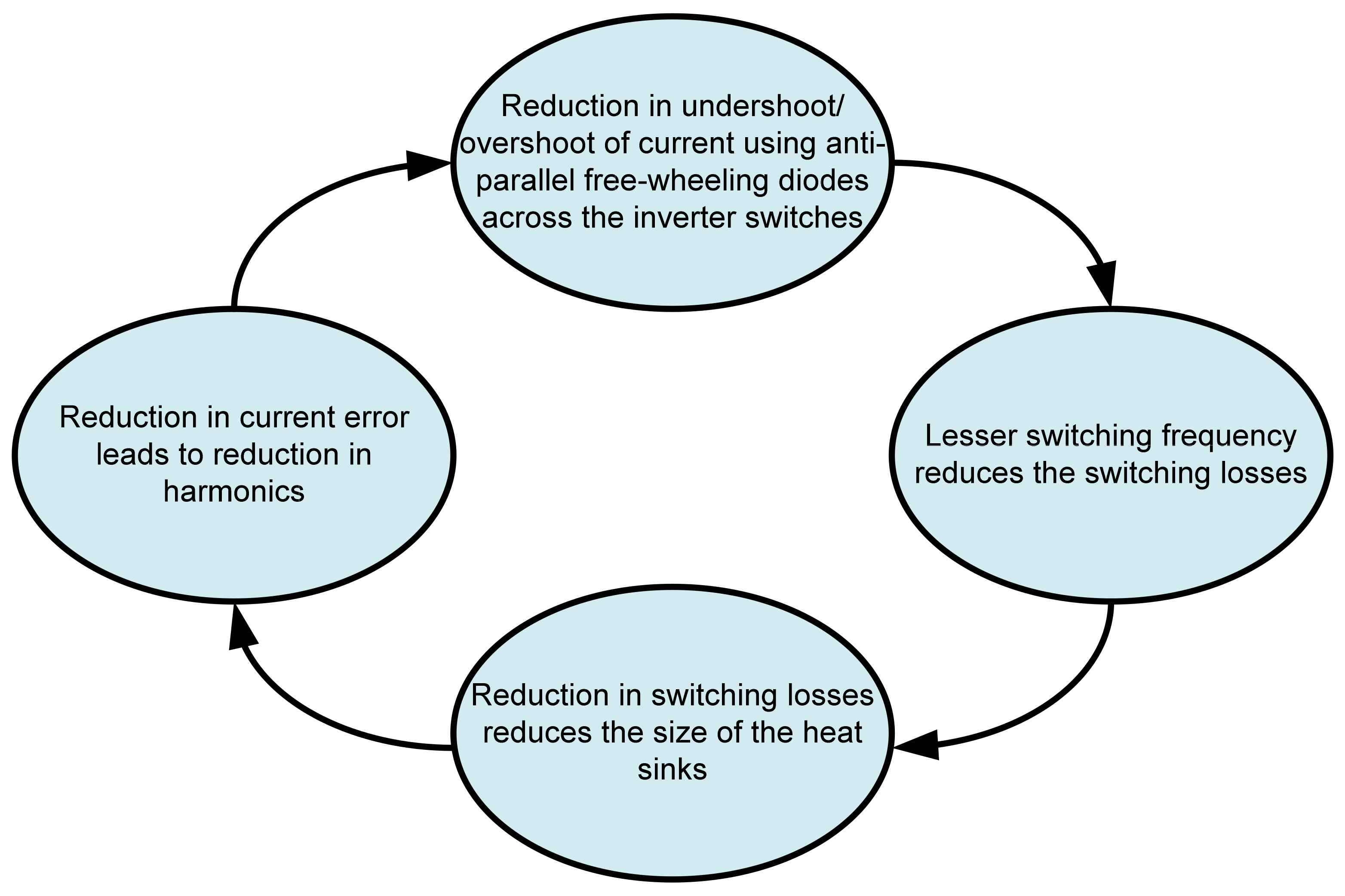
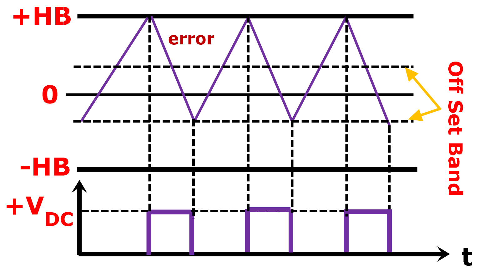
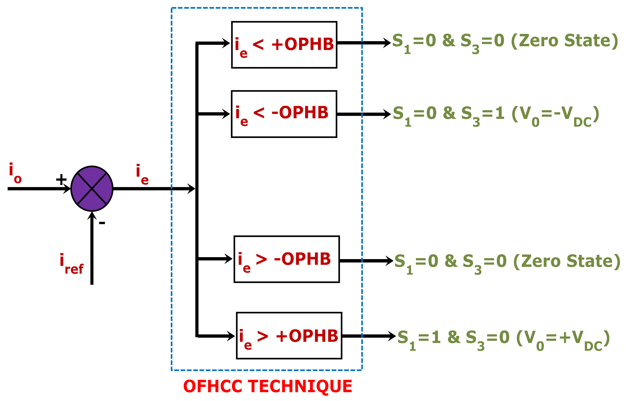
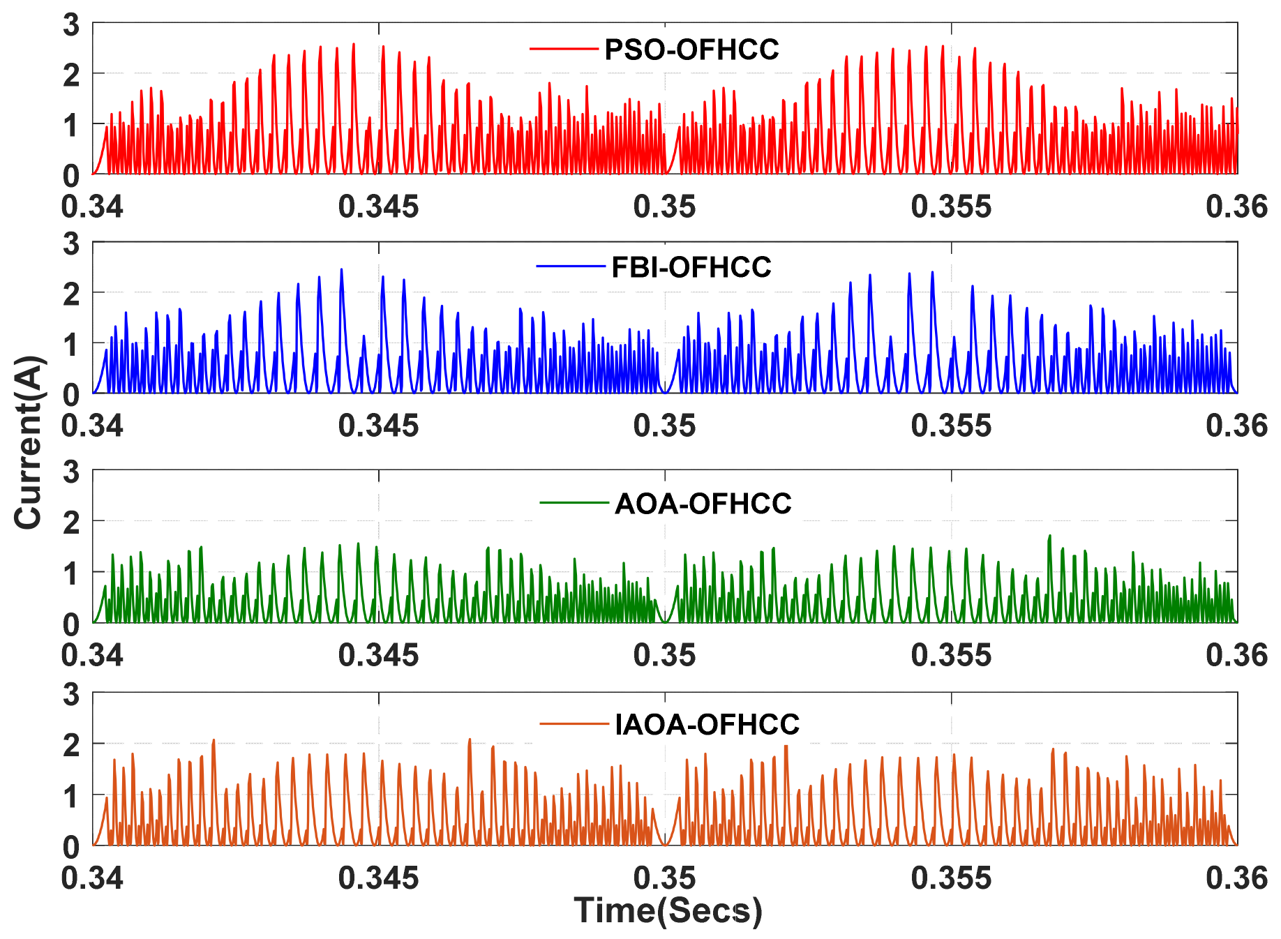
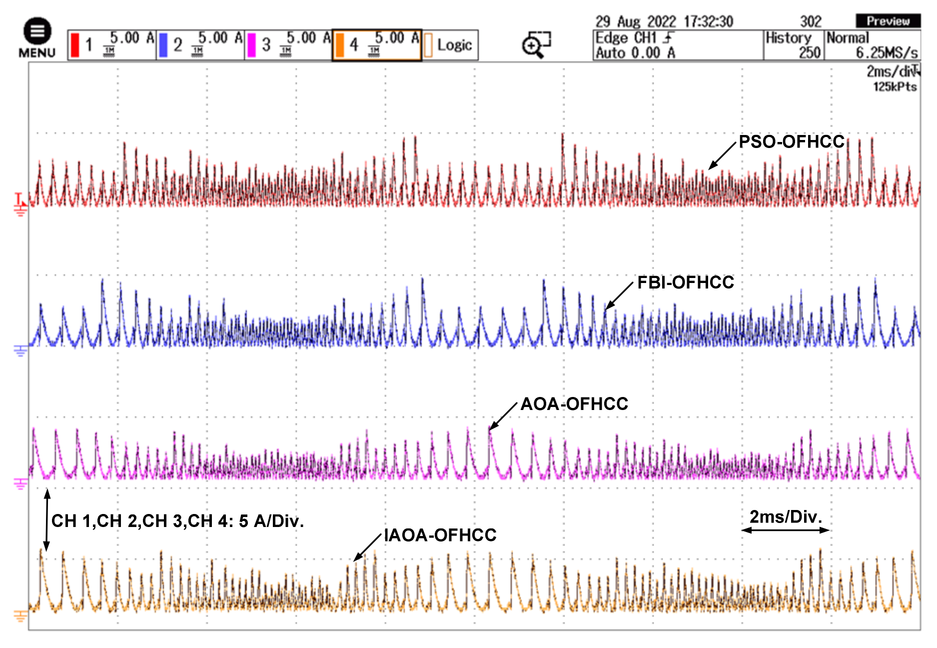
3.2. Offset Hysteresis Band Current Controller (OFHCC)
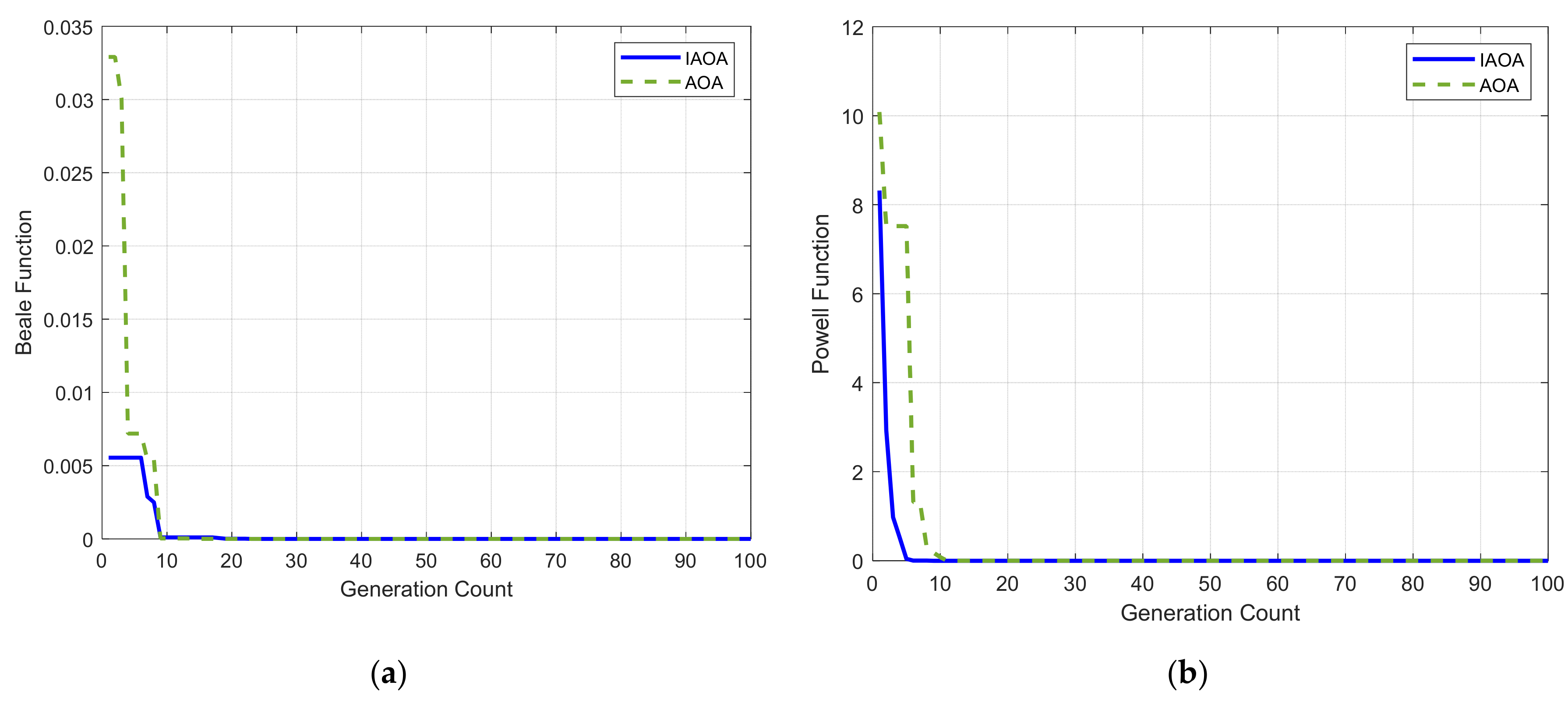
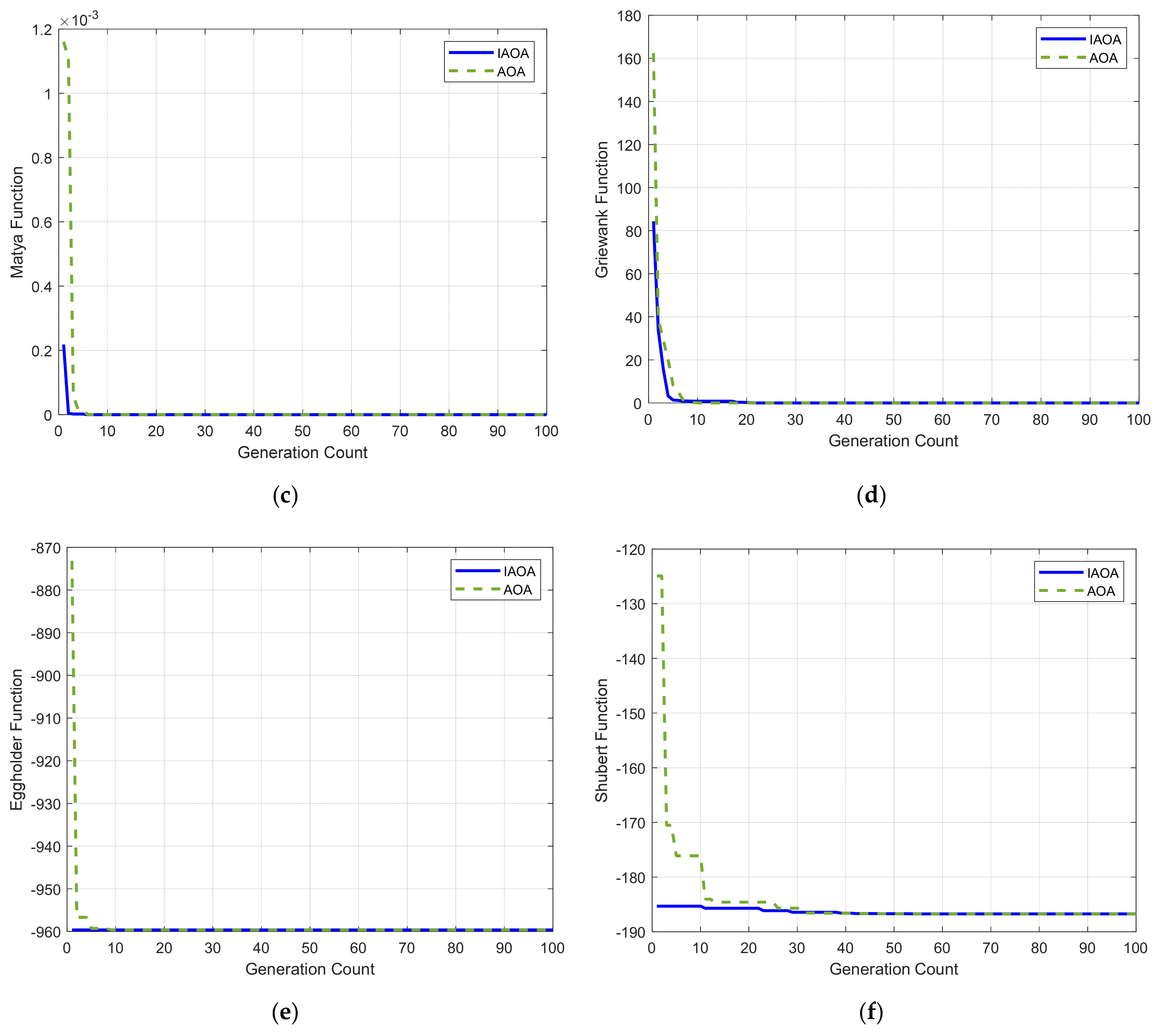
4. Common Benchmark Functions Used in the Study
5. Analysis of Algorithms
5.1. Forensic-Based Investigation (FBI) Algorithm
| = effectiveness coefficient, i.e., [−1, 1]; | lowest possibility value corresponding to the worst objective value; |
| j = 1, 2, …, D, and D is the number of dimensions; | highest possibility position corresponding to the best objective value; |
| are the numbers of individuals that affect the movement of assumed to be 2 and 3; | = possibility that the suspect is at location ; |
| d, k, h, and i are four suspected locations; {d, k, h, i} ε {1, 2, …, NP}; d, k, and h are chosen randomly; and NP is the number of suspected locations; | highest possibility position corresponding to the best solution; |
| = suspected location; | rand is a random number in the range [−1, 1]; |
| = new suspected location; | rand1, rand2, rand3, and rand4 are random numbers in the range [0, 1]. |
5.2. Particle Swarm Optimization (PSO) Algorithm
- 1.
- Initialization: Within the specific search range, the initial population and initial size velocity [NP × D] are generated. Here, ‘D’ is the dimension of the problem and ‘NP’ is the number of the population.
- 2.
- Velocity update: Equation (19) is utilized to update the velocity in this step.where ‘C1′ and ‘C2′ are acceleration constants generally taken as 2.05; pbest is the local best, i.e., the best solution so far achieved by a particle; gbest is the global best i.e., the best solution in the population; rand1 and rand2 are random numbers within the range [0, 1]; and ‘w’ is called the inertia weight, which is decreased from 0.9 to 0.4 with iterations.
- 3.
- Position update: The newly generated velocity is combined with the initial population to update the initial population.
5.3. Arithmetic Optimization Algorithm (AOA)
- 1.
- Initialization: The initial population size [NP × D] is developed randomly within the predefined search space. Equation (21) evaluates the math optimizer acceleration (MOA).where ‘iter’ and ‘itermax’ are the iteration count and the maximum number of iterations; ‘mina’ and ‘maxa’ are the minimum and maximum values of the acceleration function taken as 0.2 and 0.9, respectively.
- 2.
- Update phase: Using Equation (22), the math optimizer probability (MOP) is generated.where the solution is updated by generating three random numbers, r1, r2, and r3, and ‘α’ is taken as 5.if r1 < MOAif r2 > 0.5elseendelseif r3 < 0.5elseendwhere ‘’ and ‘’are the upper and lower limits of the variables to be designed and ‘’ is taken as 0.5.
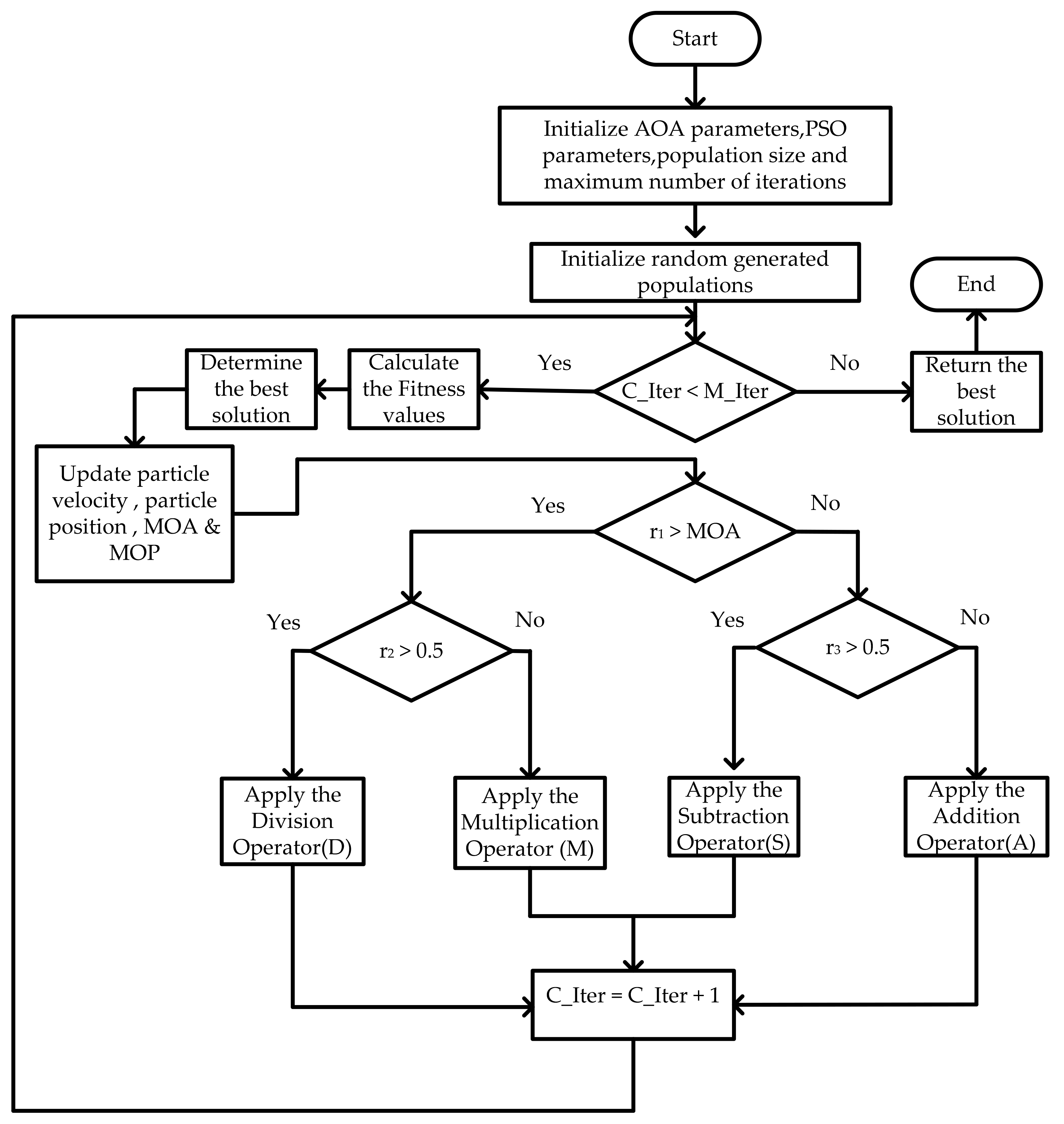
5.4. Improved Arithmetic Optimization Algorithm (IAOA)
- Generate the initial population for design variables and the constants ‘’ of the AOA technique.
- Evaluate the objective function and identify the best-performing solution (gbest).
- Update the solution with the AOA technique using Equations (21)–(26).
- Update the values of ‘’ with the PSO algorithm using Equations (19) and (20).
- Repeat the previous two steps until the stopping criterion is met.
6. Results and Discussion
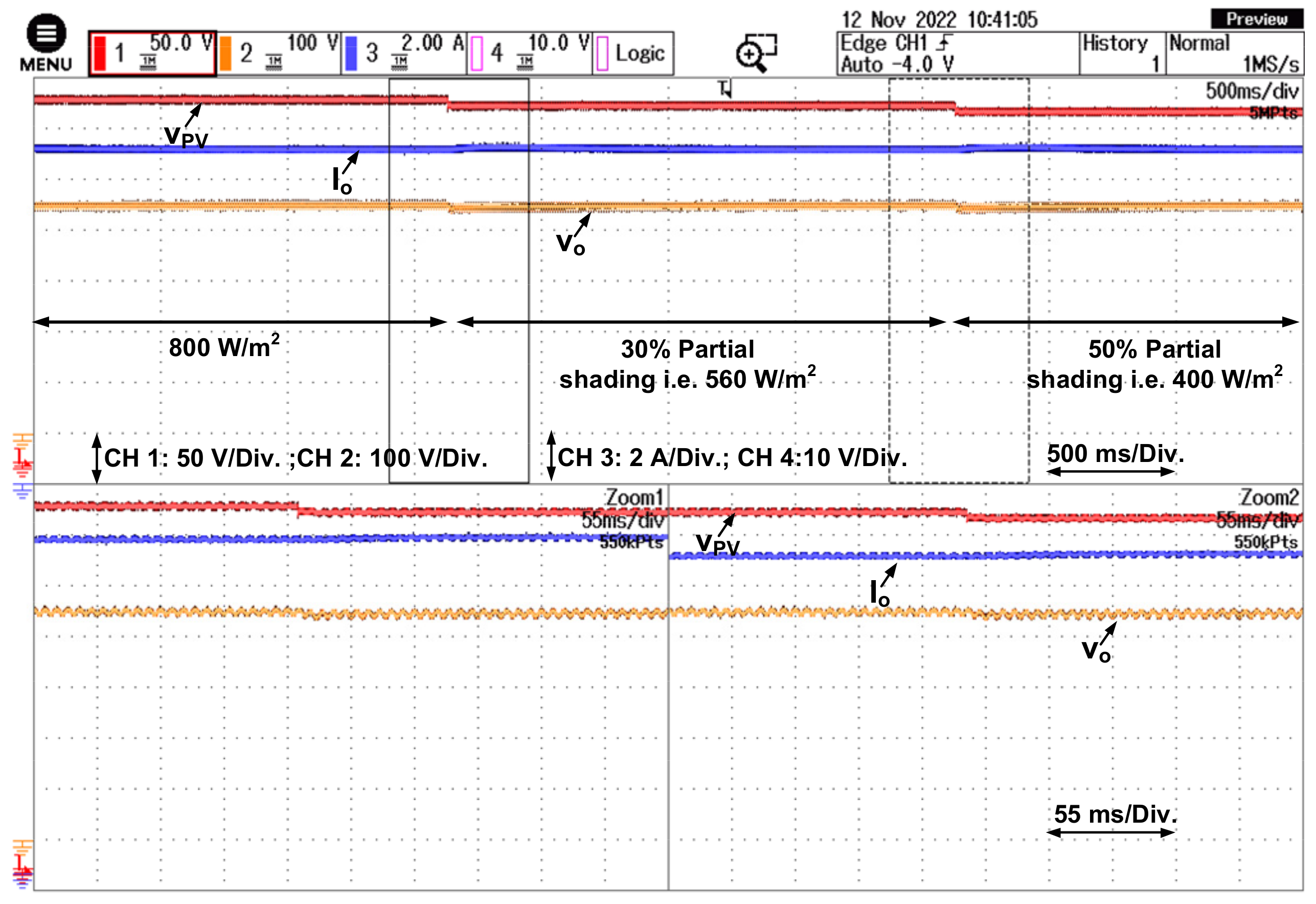
Behavior of the Proposed Control Algorithm under Partial Shading Condition
7. Conclusions
Author Contributions
Funding
Data Availability Statement
Acknowledgments
Conflicts of Interest
References
- Bastida, L.; Cohen, J.J.; Kollmann, A.; Moya, A.; Reichl, J. Exploring the role of ICT on household behavioural energy efficiency to mitigate global warming. Renew. Sustain. Energy Rev. 2019, 103, 455–462. [Google Scholar] [CrossRef] [Green Version]
- Al-Shetwi, A.Q.; Hannan, M.A.; Jern, K.P.; Mansur, M.; Mahlia, T.M. Grid-connected renewable energy sources: Review of the recent integration requirements and control methods. J. Clean. Prod. 2020, 253, 119831. [Google Scholar] [CrossRef]
- Irena, I. Renewable Power Generation Costs in 2017; Report; International Renewable Energy Agency: Abu Dhabi, United Arab Emirates, 2018. [Google Scholar]
- Bhandari, B.; Lee, K.T.; Lee, G.Y.; Cho, Y.M.; Ahn, S.H. Optimization of hybrid renewable energy power systems: A review. Int. J. Precis. Eng. Manuf.-Green Technol. 2015, 2, 99–112. [Google Scholar] [CrossRef]
- Lund, H.; Mathiesen, B.V. Energy system analysis of 100% renewable energy systems—The case of Denmark in years 2030 and 2050. Energy 2009, 34, 524–531. [Google Scholar] [CrossRef]
- Harrouz, A.; Abbes, M.; Colak, I.; Kayisli, K. Smart grid and renewable energy in Algeria. In Proceedings of the IEEE 6th International Conference on Renewable Energy Research and Applications (ICRERA), San Diego, CA, USA, 5–8 November 2017; pp. 1166–1171. [Google Scholar]
- Qazi, A.; Hussain, F.; Rahim, N.A.; Hardaker, G.; Alghazzawi, D.; Shaban, K.; Haruna, K. Towards sustainable energy: A systematic review of renewable energy sources, technologies, and public opinions. IEEE Access 2019, 7, 63837–63851. [Google Scholar] [CrossRef]
- Al Maamary, H.M.; Kazem, H.A.; Chaichan, M.T. Renewable energy and GCC States energy challenges in the 21st century: A review. Int. J. Comput. Appl. Sci. IJOCAAS 2017, 2, 11–18. [Google Scholar]
- Hannan, M.A.; Ghani, Z.A.; Hoque, M.M.; Hossain Lipu, M.S. A fuzzy-rule-based PV inverter controller to enhance the quality of solar power supply: Experimental test and validation. Electronics 2019, 8, 1335. [Google Scholar] [CrossRef] [Green Version]
- Gul, M.; Kotak, Y.; Muneer, T. Review on recent trend of solar photovoltaic technology. Energy Explor. Exploit. 2016, 34, 485–526. [Google Scholar] [CrossRef] [Green Version]
- Sathishkumar, R.; Malathi, V.; Premka, V. Optimization and design of PV-wind hybrid system for DC micro grid using NSGA II. Circuits Syst. 2016, 7, 1106. [Google Scholar] [CrossRef] [Green Version]
- Sawant, P.T.; Bhattar, C.L. Optimization of PV system using particle swarm algorithm under dynamic weather conditions. In Proceedings of the IEEE 6th International Conference on Advanced Computing (IACC), Bhimavaram, India, 27–28 February 2016; pp. 208–213. [Google Scholar]
- Ram, J.P.; Babu, T.S.; Rajasekar, N. A comprehensive review on solar PV maximum power point tracking techniques. Renew. Sustain. Energy Rev. 2017, 67, 826–847. [Google Scholar] [CrossRef]
- Zakaria, A.; Ismail, F.B.; Lipu, M.H.; Hannan, M.A. Uncertainty models for stochastic optimization in renewable energy applications. Renew. Energy 2020, 145, 1543–1571. [Google Scholar] [CrossRef]
- Hannan, M.A.; Tan, S.Y.; Al-Shetwi, A.Q.; Jern, K.P.; Begum, R.A. Optimized controller for renewable energy sources integration into micro-grid: Functions, constraints and suggestions. J. Clean. Prod. 2020, 256, 120419. [Google Scholar] [CrossRef]
- Ilas, A.; Ralon, P.; Rodriguez, A.; Taylor, M. Renewable Power Generation Costs; International Renewable Energy Agency: Abu Dhabi, United Arab Emirates, 2017. [Google Scholar]
- Gooding, P.A.; Makram, E.; Hadidi, R. Probability analysis of distributed generation for island scenarios utilizing Carolinas data. Electr. Power Syst. Res. 2014, 107, 125–132. [Google Scholar] [CrossRef]
- Blondeau, J.; Mertens, J. Impact of intermittent renewable energy production on specific CO2 and NOx emissions from large scale gas-fired combined cycles. J. Clean. Prod. 2019, 221, 261–270. [Google Scholar] [CrossRef]
- Khishe, M.; Mosavi, M.R. Chimp optimization algorithm. Expert Syst. Appl. 2020, 149, 113338. [Google Scholar] [CrossRef]
- Eberhat, R.; Kennedy, J. A new optimizer using particle swarm theory. In Proceedings of the Sixth International Symposium on Micro Machine and Human Science, Piscataway, NJ, USA, 4–6 October 1995; pp. 39–43. [Google Scholar]
- Mirjalili, S.; Mirjalili, S.M.; Lewis, A. Grey Wolf Optimizer. Adv. Eng. Softw. 2014, 69, 46–61. [Google Scholar] [CrossRef] [Green Version]
- Rao, R.V.; Savsani, V.J.; Vakharia, D.P. Teaching–learning-based optimization: A novel method for constrained mechanical design optimization problems. Comput.-Aided Des. 2011, 43, 303–315. [Google Scholar] [CrossRef]
- Xiang, W.L.; An, M.Q. An efficient and robust artificial bee colony algorithm for numerical optimization. Comput. Oper. Res. 2013, 40, 1256–1265. [Google Scholar] [CrossRef]
- Abualigah, L.; Diabat, A.; Mirjalili, S.; Abd Elaziz, M.; Gandomi, A.H. The arithmetic optimization algorithm. Comput. Methods Appl. Mech. Eng. 2021, 376, 113609. [Google Scholar] [CrossRef]
- Varaprasad, O.V.; Sarma, D.S. An improved three level Hysteresis Current Controller for single phase shunt active power filter. In Proceedings of the IEEE 6th India International Conference on Power Electronics, Kurukshetra, India, 8–10 December 2014; pp. 1–5. [Google Scholar]
- Zeb, K.; Uddin, W.; Adil Khan, M.; Ali, Z.; Umair Ali, M.; Christofides, N.; Kim, H.J. A comprehensive review on inverter topologies and control strategies for grid connected photovoltaic system. Renew. Sustain. Energy Rev. 2018, 94, 1120–1141. [Google Scholar] [CrossRef]
- Parvez, M.; Elias, M.F.M.; Rahim, N.A.; Osman, N. Current control techniques for three-phase grid interconnection of renewable power generation systems: A review. Sol. Energy 2016, 135, 29–42. [Google Scholar] [CrossRef]
- Hassan, Z.; Amir, A.; Selvaraj, J.; Rahim, N.A. A review on current injection techniques for low-voltage ride-through and grid fault conditions in grid-connected photovoltaic system. Sol. Energy 2020, 207, 851–873. [Google Scholar] [CrossRef]
- Tian, H.; Mancilla David, F.; Ellis, K.; Muljadi, E.; Jenkins, P.A. Cell-to-module-to-array detailed model for photovoltaic panels. Sol. Energy 2012, 86, 2695–2706. [Google Scholar] [CrossRef]
- Vengatesh, R.P.; Rajan, S.E. Investigation of cloudless solar radiation with PV module employing Matlab-Simulink. In Proceedings of the International Conference on Emerging Trends in Electrical and Computer Technology, Nagercoil, India, 23–24 March 2011; pp. 141–147. [Google Scholar]
- Zhang, Y.; Gao, S.; Gu, T. Prediction of IV characteristics for a PV panel by combining single diode model and explicit analytical model. Sol. Energy 2017, 144, 349–355. [Google Scholar] [CrossRef]
- Jalil, M.F.; Khatoon, S.; Nasiruddin, I.; Bansal, R.C. Review of PV array modelling, configuration and MPPT techniques. Int. J. Model. Simul. 2022, 42, 533–550. [Google Scholar] [CrossRef]
- Koutroulis, E.; Blaabjerg, F. Methodology for the optimal design of transformer less grid-connected PV inverters. IET Power Electron. 2012, 5, 1491–1499. [Google Scholar] [CrossRef] [Green Version]
- Reddak, M. An improved control strategy using RSC of the wind turbine based on DFIG for grid harmonic currents mitigation. Int. J. Renew. Energy Res. (IJRER) 2018, 8, 266–273. [Google Scholar]
- Sharma, S.; Singh, B. Control of permanent magnet synchronous generator-based stand-alone wind energy conversion system. IET Power Electron. 2012, 5, 1519–1526. [Google Scholar] [CrossRef]
- Kean, Y.W.; Ramasamy, A.; Sukumar, S.; Marsadek, M. Adaptive controllers for enhancement of stand-alone hybrid system performance. Int. J. Power Electron. Drive Syst. 2018, 9, 979. [Google Scholar] [CrossRef]
- Panda, A.; Pathak, M.K.; Srivastava, S.P. A single phase photovoltaic inverter control for grid connected system. Sadhana 2016, 41, 15–30. [Google Scholar] [CrossRef] [Green Version]
- Reddak, M.; Mesbahi, A.; Nouaiti, A.; Berdai, A. Design and implementation of nonlinear integral back stepping control strategy for single-phase grid-connected VSI. Int. J. Power Electron. Drive Syst. 2019, 10, 19. [Google Scholar]
- Dyga, Ł.; Rymarski, Z.; Bernacki, K. The wavelet-aided methods for evaluating the output signal that is designated for uninterruptible power supply systems. Przegląd Elektrotechniczny 2020, 96, 50–54. [Google Scholar] [CrossRef]
- Rymarski, Z.; Bernacki, K. Different Features of Control Systems for Single-Phase Voltage Source Inverters. Energies 2020, 13, 4100. [Google Scholar] [CrossRef]
- Torrey, D.; Al-Zamel, A. Single-phase active power filters for multiple nonlinear loads. IEEE Trans. Power Electron. 1995, 10, 263–272. [Google Scholar] [CrossRef]
- Abd Rahim, N.; Selvaraj, J. Implementation of hysteresis current control for single-phase grid connected inverter. In Proceedings of the International Conference on Power Electronics and Drive Systems, Bangkok, Thailand, 27–30 November 2007; pp. 1097–1101. [Google Scholar]
- Dahono, P.A. New hysteresis current controller for single-phase full-bridge inverters. IET Power Electron. 2009, 2, 585–594. [Google Scholar] [CrossRef]
- Yao, Z.; Xiao, L. Control of single-phase grid-connected inverters with nonlinear loads. IEEE Trans. Ind. Electron. 2011, 60, 1384–1389. [Google Scholar] [CrossRef]
- Elsaharty, M.A.; Hamad, M.S.; Ashour, H.A. Digital hysteresis current control for grid-connected converters with LCL filter. In Proceedings of the 37th Annual Conference of the IEEE Industrial Electronics Society, Melbourne, Australia, 7–10 November 2011; pp. 4685–4690. [Google Scholar]
- Ichikawa, R.; Funato, H.; Nemoto, K. Experimental verification of single phase utility interface inverter based on digital hysteresis current controller. In Proceedings of the International Conference on Electrical Machines and Systems, Beijing, China, 20–23 August 2011; pp. 1–6. [Google Scholar]
- Chatterjee, A.; Mohanty, K.B. Current control strategies for single phase grid integrated inverters for photovoltaic applications-a review. Renew. Sustain. Energy Rev. 2018, 92, 554–569. [Google Scholar] [CrossRef]
- Jena, S.; Mohapatra, B.; Panigrahi, C.K.; Mohanty, S.K. Power quality improvement of 1-φ grid integrated pulse width modulated voltage source inverter using hysteresis Current Controller with offset band. In Proceedings of the 3rd International Conference on Advanced Computing and Communication Systems (ICACCS), Coimbatore, India, 22–23 January 2016; pp. 1–7. [Google Scholar] [CrossRef]
- Karuppanan, P.; Ram, S.K.; Mahapatra, K. Three level hysteresis current controller based active power filter for harmonic compensation. In Proceedings of the International Conference on Emerging Trends in Electrical and Computer Technology, Nagercoil, India, 23–24 March 2011; pp. 407–412. [Google Scholar]
- Yang, X.S. Nature-Inspired Optimization Algorithms; Academic Press: Cambridge, MA, USA, 2020. [Google Scholar]
- Gupta, S.; Deep, K.; Mirjalili, S. An efficient equilibrium optimizer with mutation strategy for numerical optimization. Appl. Soft Comput. 2020, 96, 106542. [Google Scholar] [CrossRef]
- Chauhan, S.; Vashishtha, G. Mutation-based arithmetic optimization algorithm for global optimization. In Proceedings of the International Conference on Intelligent Technologies (CONIT), Hubli, India, 25–27 June 2021; pp. 1–6. [Google Scholar]
- Chou, J.S.; Nguyen, N.M. FBI inspired meta-optimization. Appl. Soft Comput. 2020, 93, 106339. [Google Scholar] [CrossRef]
- Salet, R. Framing in criminal investigation: How police officers (re) construct a crime. Police J. 2017, 90, 128–142. [Google Scholar] [CrossRef] [Green Version]
- Fathy, A.; Rezk, H.; Alanazi, T.M. Recent approach of forensic-based investigation algorithm for optimizing fractional order PID-based MPPT with proton exchange membrane fuel cell. IEEE Access 2021, 9, 18974–18992. [Google Scholar] [CrossRef]
- Wang, D.; Tan, D.; Liu, L. Particle swarm optimization algorithm: An overview. Soft Comput. 2018, 22, 387–408. [Google Scholar] [CrossRef]
- Hasari, S.A.; Salemnia, A.; Hamzeh, M. Applicable method for average switching loss calculation in power electronic converters. J. Power Electron. 2017, 17, 1097–1108. [Google Scholar]
- Singh, J.K.; Behera, R.K. Hysteresis current controllers for grid connected inverter: Review and experimental implementation. In Proceedings of the IEEE International Conference on Power Electronics, Drives and Energy Systems (PEDES), Chennai, India, 18–21 December 2018; pp. 1–6. [Google Scholar]


| Function | Function’s Expression | Dimension | Range |
|---|---|---|---|
| Beale (F1) | 2 | [−4.5, 4.5] | |
| Powell (F2) | 10 | [−4, 5] | |
| Matyas (F3) | 2 | [−10, 10] | |
| Griewank (F4) | 30 | [−600, 600] | |
| Eggholder (F5) | 2 | [−512, 512] | |
| Shubert (F6) | 2 | [−5.12, 5.12] |
| Algorithm | Function | Optimum Value | Minimum | Maximum | Mean | Standard Deviation | Computational Time (s) |
|---|---|---|---|---|---|---|---|
| IAOA | F1 | 0 | 3.5828 × 10⁻¹⁶ | 1.9598 × 10⁻¹³ | 4.2215 × 10⁻¹⁴ | 4.9633 × 10⁻¹⁴ | 0.0834 |
| AOA | 1.0785 × 10⁻¹⁵ | 7.7380 × 10⁻¹³ | 8.6741 × 10⁻¹⁴ | 1.7924 × 10⁻¹³ | 0.0595 | ||
| IAOA | F2 | 0 | 0 | 2.6215 × 10⁻²⁰ | 8.7385 × 10⁻²² | 4.7863 × 10⁻²¹ | 0.0766 |
| AOA | 0 | 6.5352 × 10⁻¹⁸ | 2.2641 × 10⁻¹⁹ | 1.1925 × 10⁻¹⁸ | 0.0563 | ||
| IAOA | F3 | 0 | 0 | 1.1962 × 10−63 | 3.9877 × 10−65 | 2.1840 × 10−64 | 0.0542 |
| AOA | 0 | 5.6773 × 10−63 | 1.8930 × 10−64 | 1.0365 × 10−63 | 0.0423 | ||
| IAOA | F4 | 0 | 0 | 0 | 0 | 0 | 0.6315 |
| AOA | 0 | 0 | 0 | 0 | 0.5263 | ||
| IAOA | F5 | −959.640 | −959.4607 | −959.4607 | −959.4607 | 1.0283 × 10⁻¹² | 0.0457 |
| AOA | −959.4607 | −959.4607 | −959.4607 | 2.0283 × 10⁻¹² | 0.0133 | ||
| IAOA | F6 | −186.731 | −186.7309 | −186.7309 | −186.7301 | 1.4597 × 10⁻⁹ | 0.0958 |
| AOA | −186.7309 | −186.7305 | −186.7309 | 8.2884 × 10⁻⁴ | 0.0757 |
| Parameter | Numerical Value |
|---|---|
| Grid frequency | 50 Hz |
| Line inductance | 15 mH |
| Irradiance | 500 W/m2 |
| 2.2 mJ | |
| 1.7 mJ | |
| Cell temperature | 25 °C |
| Load variation | 1000 W to 2000 W |
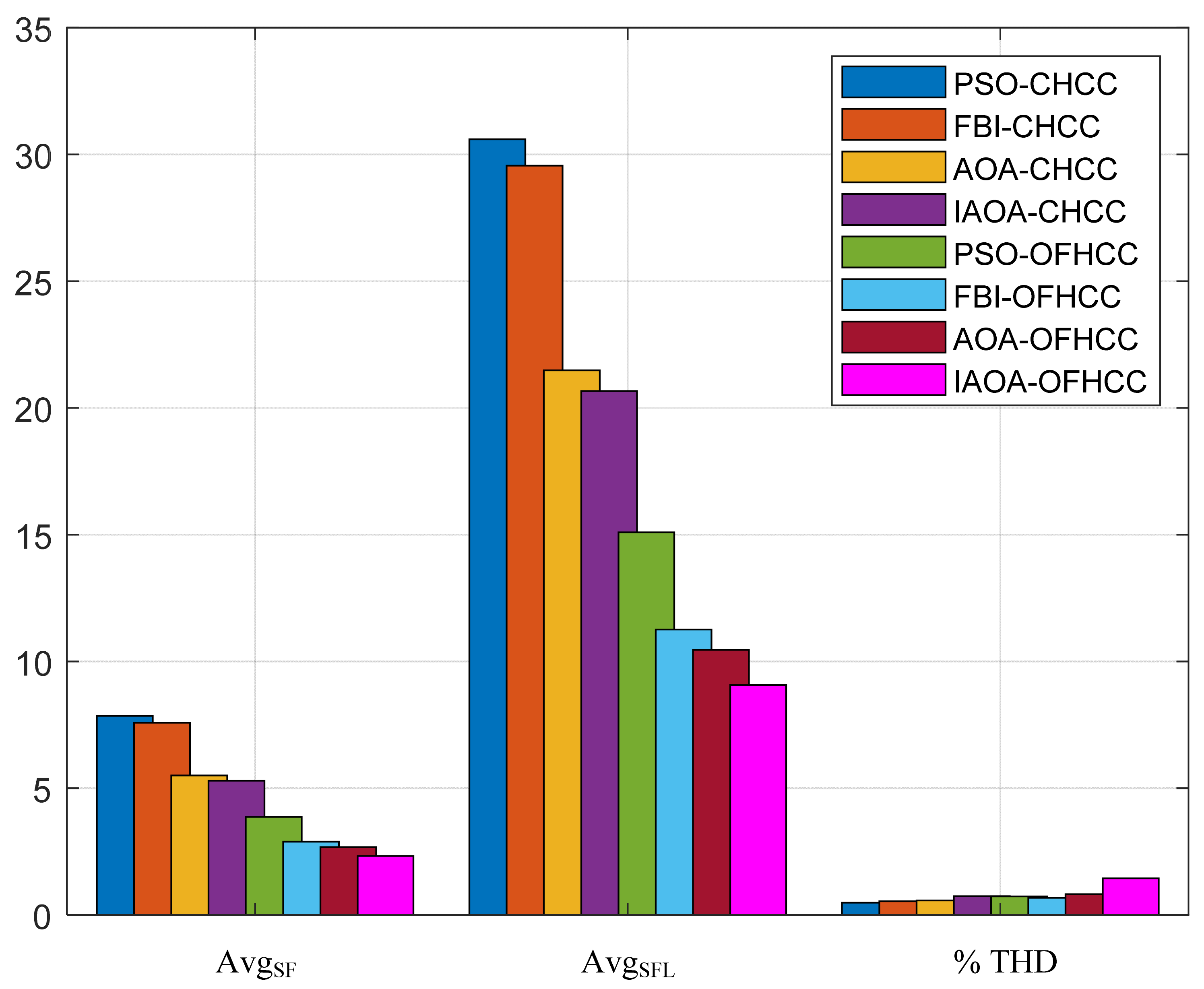
| Controller | D | HB1 | HB2 | HB3 | HB4 | MaxSF (in kHz) | MinSF (in kHz) | AvgSF (in kHz) | AvgSFL (in W) | ZSF (in kHz) | %THD |
|---|---|---|---|---|---|---|---|---|---|---|---|
| PSO-CHCC | 0.215 | 0.375 | −0.572 | - | - | 9.25 | 8.75 | 7.85 | 30.60 | 8.50 | 0.49 |
| FBI-CHCC | 0.319 | 0.462 | −0.868 | - | - | 8.75 | 6.25 | 7.58 | 29.56 | 8.00 | 0.54 |
| AOA-CHCC | 0.169 | 0.620 | −0.587 | - | - | 7.25 | 3.25 | 5.50 | 21.48 | 6.50 | 0.57 |
| IAOA-CHCC | 0.245 | 0.809 | −0.932 | - | - | 6.25 | 3.75 | 5.30 | 20.67 | 5.75 | 0.74 |
| PSO-OFHCC | 0.279 | 0.953 | −0.874 | 0.874 | −0.953 | 6 | 3.50 | 3.87 | 15.09 | 4.25 | 0.73 |
| FBI-OFHCC | 0.112 | 0.913 | −0.827 | 0.827 | −0.913 | 5.5 | 2.50 | 2.89 | 11.26 | 3.25 | 0.68 |
| AOA-OFHCC | 0.141 | 0.817 | −0.645 | 0.645 | −0.817 | 6 | 2.75 | 2.68 | 10.46 | 3.75 | 0.82 |
| IAOA-OFHCC | 0.117 | 0.964 | −0.532 | 0.532 | −0.964 | 6.25 | 2.75 | 2.33 | 9.07 | 3.50 | 1.45 |
| SBHCC [58] | - | 0.5 | −0.5 | - | - | 20 | - | - | - | - | 4.42 |
| DBHCC−1 [58] | - | 0.5 | −0.5 | - | - | 10 | - | - | - | - | 4.33 |
| DBHCC−2 [58] | - | 0.5 | −0.5 | - | - | 20 | - | - | - | - | 2.65 |
| MDBHCC [58] | - | 0.5 | −0.5 | - | - | 5.5 | - | - | - | - | 4.33 |
| VBHCC [58] | - | 0.5 | −0.5 | - | - | 15 | - | - | - | - | 4.17 |
Publisher’s Note: MDPI stays neutral with regard to jurisdictional claims in published maps and institutional affiliations. |
© 2022 by the authors. Licensee MDPI, Basel, Switzerland. This article is an open access article distributed under the terms and conditions of the Creative Commons Attribution (CC BY) license (https://creativecommons.org/licenses/by/4.0/).
Share and Cite
Mohapatra, B.; Sahu, B.K.; Pati, S.; Bajaj, M.; Blazek, V.; Prokop, L.; Misak, S.; Alharthi, M. Real-Time Validation of a Novel IAOA Technique-Based Offset Hysteresis Band Current Controller for Grid-Tied Photovoltaic System. Energies 2022, 15, 8790. https://doi.org/10.3390/en15238790
Mohapatra B, Sahu BK, Pati S, Bajaj M, Blazek V, Prokop L, Misak S, Alharthi M. Real-Time Validation of a Novel IAOA Technique-Based Offset Hysteresis Band Current Controller for Grid-Tied Photovoltaic System. Energies. 2022; 15(23):8790. https://doi.org/10.3390/en15238790
Chicago/Turabian StyleMohapatra, Bhabasis, Binod Kumar Sahu, Swagat Pati, Mohit Bajaj, Vojtech Blazek, Lukas Prokop, Stanislav Misak, and Mosleh Alharthi. 2022. "Real-Time Validation of a Novel IAOA Technique-Based Offset Hysteresis Band Current Controller for Grid-Tied Photovoltaic System" Energies 15, no. 23: 8790. https://doi.org/10.3390/en15238790
APA StyleMohapatra, B., Sahu, B. K., Pati, S., Bajaj, M., Blazek, V., Prokop, L., Misak, S., & Alharthi, M. (2022). Real-Time Validation of a Novel IAOA Technique-Based Offset Hysteresis Band Current Controller for Grid-Tied Photovoltaic System. Energies, 15(23), 8790. https://doi.org/10.3390/en15238790