
Barrier Lyapunov Function-Based Adaptive Back-Stepping Control for Electronic Throttle Control System


Abstract
1. Introduction
2. Materials and Methods
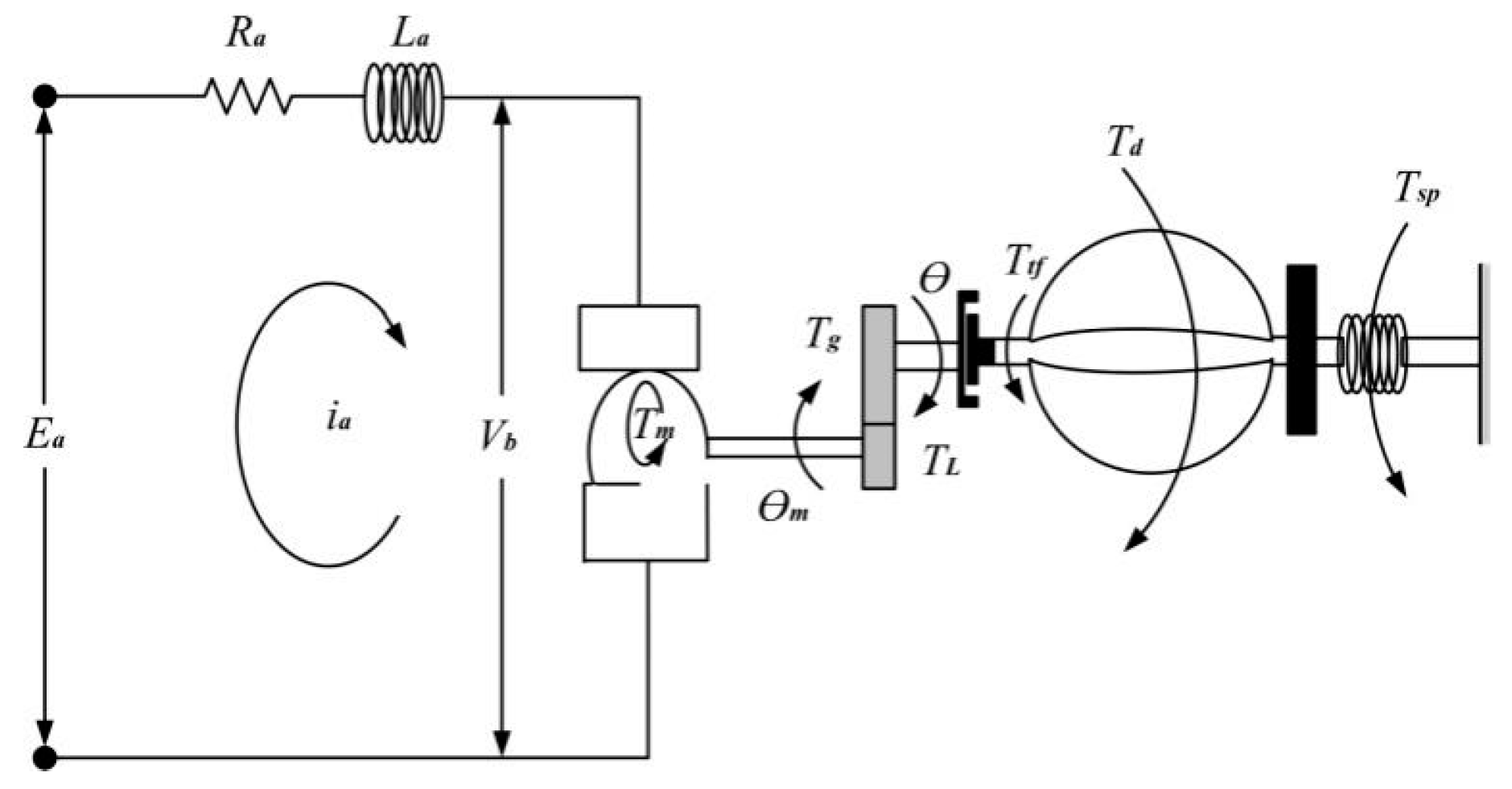
2.1. Electronic Throttle Mathematics Model
2.2. Problem Statement
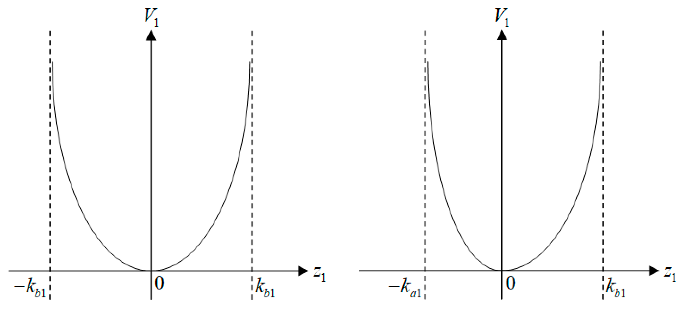
2.3. BLF Preliminaries
3. Controller Design
4. Discussion
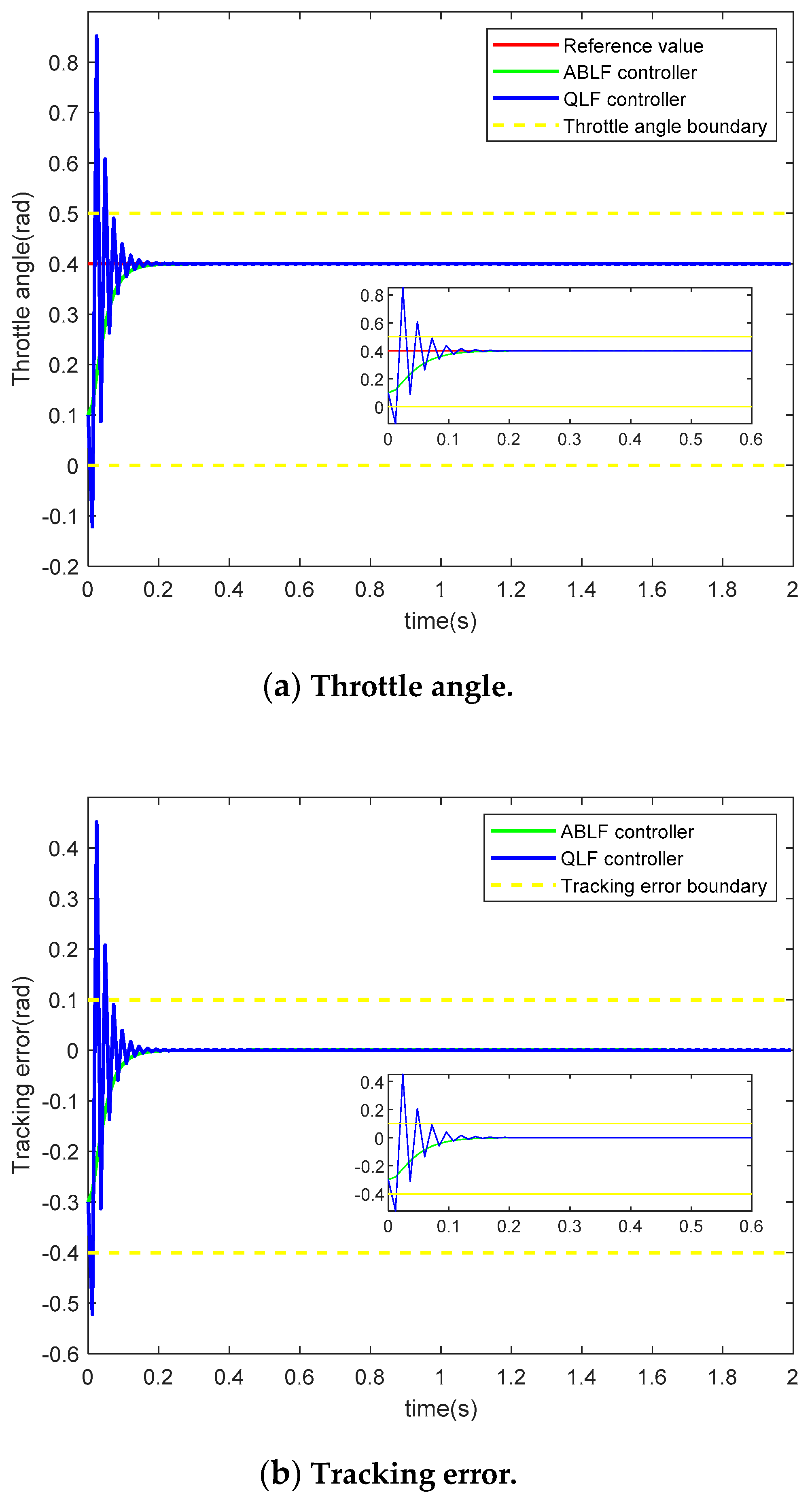
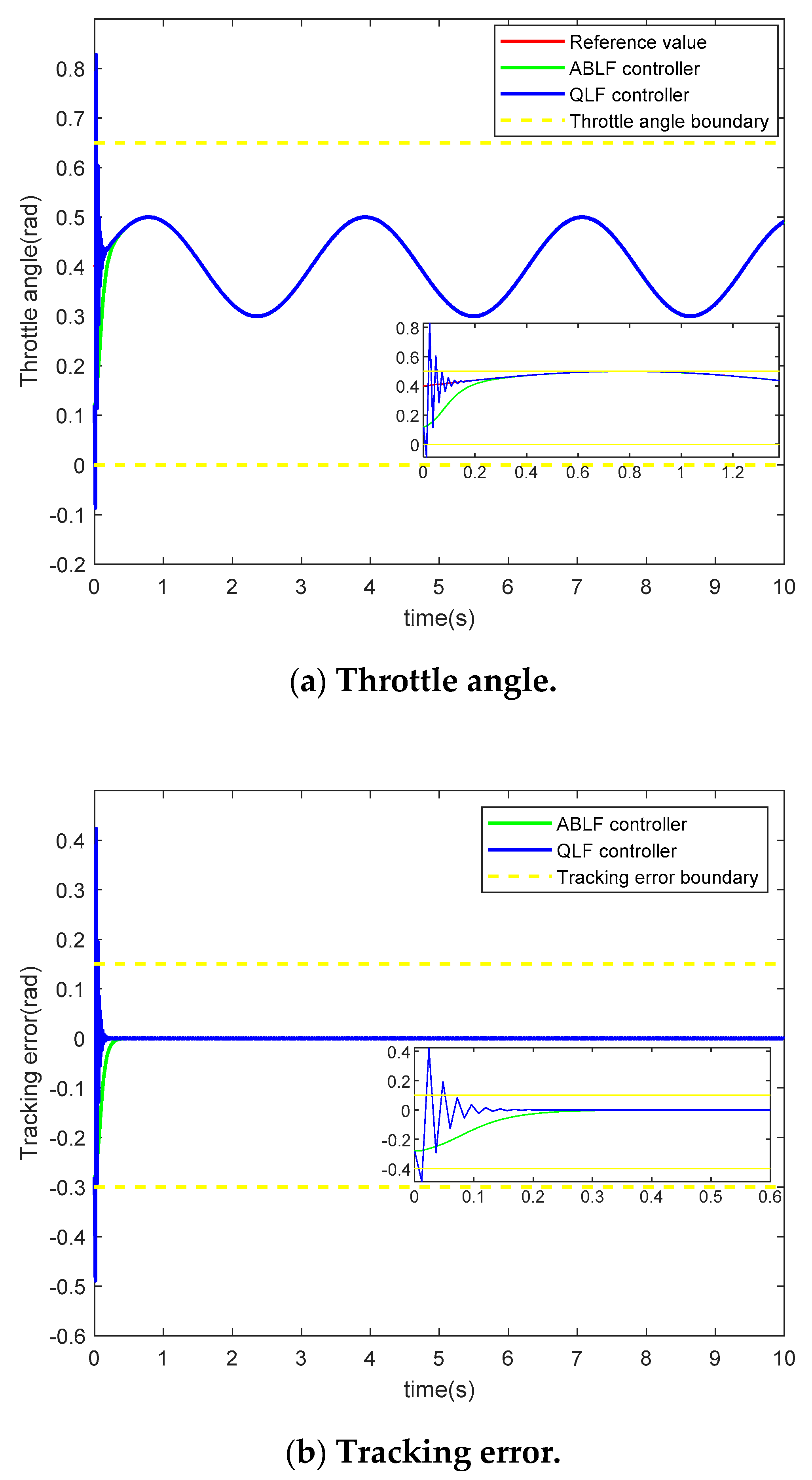
4.1. Case 1
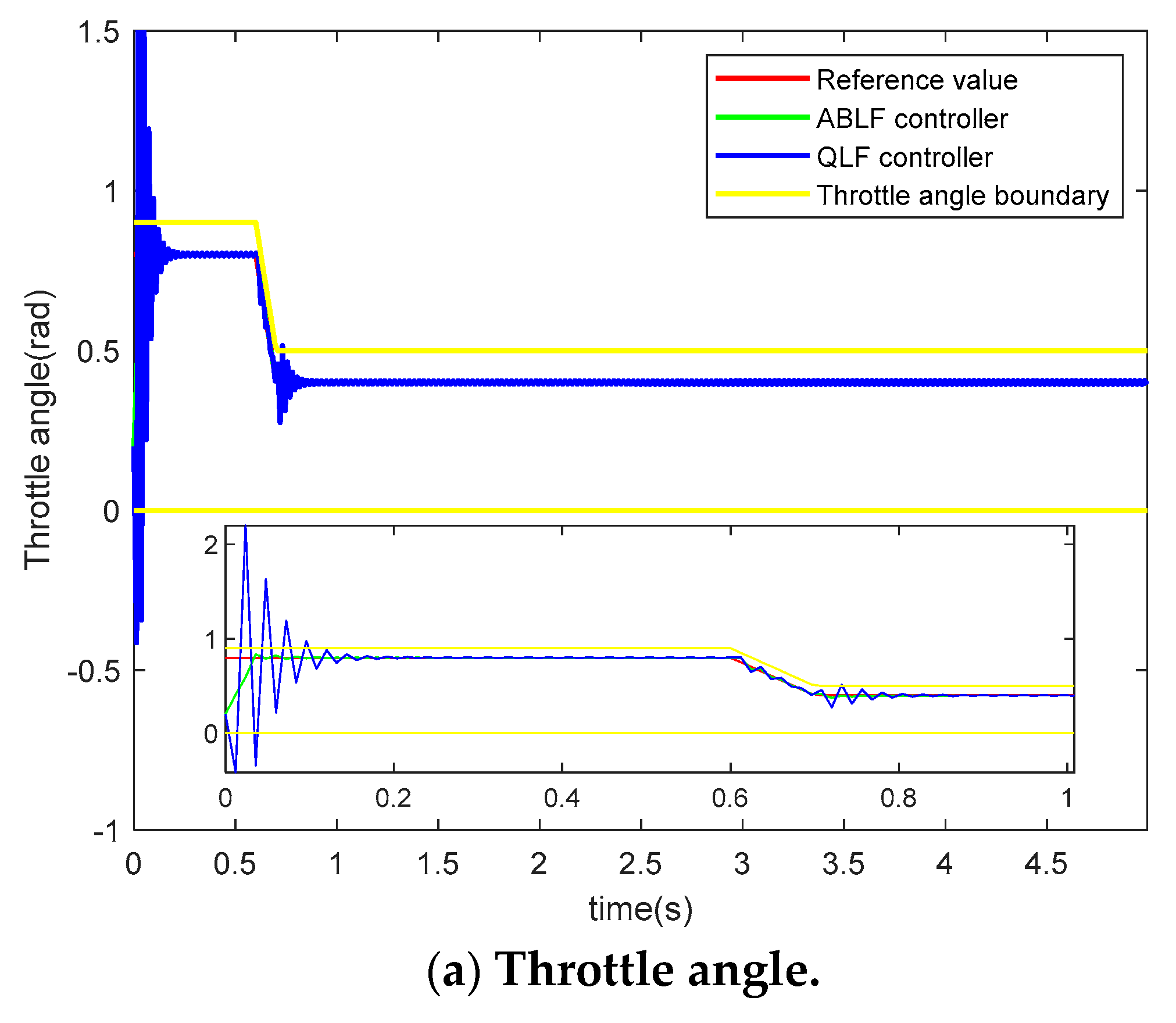
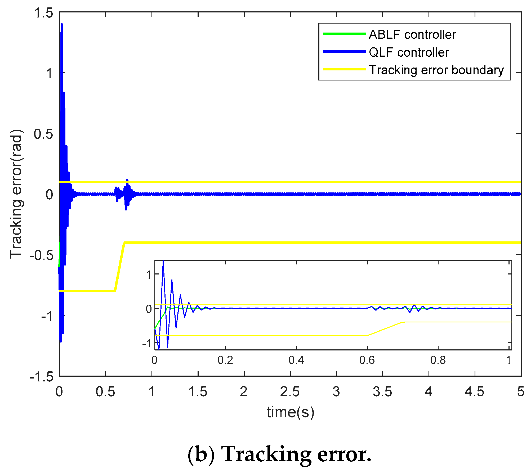
4.2. Case 2
4.3. Case 3
5. Conclusions
Author Contributions
Funding
Institutional Review Board Statement
Informed Consent Statement
Data Availability Statement
Conflicts of Interest
References
- Wang, H.; Yuan, X.; Wang, Y.; Yang, Y. Harmony search algorithm-based fuzzy-PID controller for electronic throttle valve. Neural Comput. Appl. 2013, 22, 329–336. [Google Scholar] [CrossRef]
- Li, Y.; Yang, B.; Zheng, T.; Li, Y. Extended State Observer Based Adaptive Back-Stepping Sliding Mode Control of Electronic Throttle in Transportation Cyber-Physical Systems. Math. Probl. Eng. 2015. [Google Scholar] [CrossRef]
- Ahmed, S.; Badri, A.S.; Mshari, M.H. Integral Sliding Mode Control Design for Electronic Throttle Valve. Eng. J. 2015, 11, 72–84. [Google Scholar]
- Bai, R. Adaptive Sliding-Mode Control of an Automotive Electronic Throttle in the Presence of Input Saturation Constraint. IEEE/CAA J. Autom. Sin. 2018, 5, 116–122. [Google Scholar] [CrossRef]
- Zheng, P.T.; Sun, J.M. Convergence Back-Stepping Controller Design of Electronic Throttle in Limited Time. Automob. Technol. 2018, 2018, 27–31. (In Chinese) [Google Scholar]
- Chen, H.; Hu, Y.F.; Guo, H.Z.; Song, T.-H. Control of electronic throttle based on backstepping approach. Control Theory Appl. 2011, 28, 91–496, 503. [Google Scholar]
- Nobuo, K.; Hiroyuki, Y. Adaptive Back-Stepping Control of Automotive Electronic Control Throttle. J. Softw. Eng. Appl. 2017, 10, 41–55. [Google Scholar]
- Nobuo, K. Back-Stepping Control of Automotive Electronic Throttle. In Proceedings of the SICE 2015—54th Annual Conference of the Society of Instrument and Control Engineers, Hangzhou, China, 28–30 July 2015. [Google Scholar]
- Wang, C.H.; Huang, D.Y. A New Intelligent Fuzzy Controller for Nonlinear Hysteretic Electronic Throttle in Modern Intelligent Automobiles. IEEE Trans. Ind. Electron. 2013, 60, 2332–2345. [Google Scholar] [CrossRef]
- İkbal, E.; Şahin, Y. Neural network-based fuzzy inference system for speed control of heavy duty vehicles with electronic throttle control system. Neural Comput. Appl. 2016, 28, 907–916. [Google Scholar]
- Khinchi, A.; Prasad, M.P.R. Control of electronic throttle valve using model predictive control. Int. J. Adv. Technol. Eng. Explor. 2016, 3, 118–124. [Google Scholar] [CrossRef]
- Wong, C.-K.; Lee, Y.-Y. Lane-Based Traffic Signal Simulation and Optimization for Preventing Overflow. Mathematics 2020, 8, 1368. [Google Scholar] [CrossRef]
- Paul, G.G. Embedded Software Control Design for an Electronic Throttle Body. Ph.D. Thesis, University of California, Berkekey, CA, USA, 2002. [Google Scholar]
- Ye, H.; Jiang, H.; Ma, S.; Tang, B.; Wahab, L. Linear model predictive control of automatic parking path tracking with soft constraints. Int. J. Adv. Robot. Syst. 2019, 16. [Google Scholar] [CrossRef]
- Zhang, J.; Sun, T. Disturbance observer-based sliding manifold predictive control for reentry hypersonic vehicles with multi-constraint. Proc. Inst. Mech. Eng. Part G J. Aerosp. Eng. 2016, 230, 485–495. [Google Scholar] [CrossRef]
- Hu, T.; Lin, Z.; Chen, B.M. An analysis and design method for linear systems subject to actuator saturation and disturbance. Automatica 2002, 38, 351–359. [Google Scholar] [CrossRef]
- Hu, T.; Lin, Z. Composite Quadratic Lyapunov Functions for Constrained Control Systems. IEEE Trans. Autom. Control 2003, 48, 440–450. [Google Scholar]
- Gilbert, E.; Kolmanovsky, I. Nonlinear tracking control in the presence of state and control constraints: A Generalized Reference Governor. Automatica 2002, 38, 2063–2073. [Google Scholar] [CrossRef]
- KogisoK; Hirata, K. Reference governor for constrained systems with time-varying references. Robot. Auton. Syst. 2009, 57, 289–295. [Google Scholar] [CrossRef]
- Bemporad, A.; Borrelli, F.; Morari, M. Model Predictive Control Based on Linear Programming—The Explicit Solution. IEEE Trans. Autom. Control 2002, 47, 1974–1985. [Google Scholar] [CrossRef]
- Kolmanovsky, I.V.; Druzhinina, M.; Sun, J. Speed-gradient approach to torque and air-to-fuel ratio control in DISC engines. Control Syst. Technol. IEEE Trans. 2002, 10, 671–678. [Google Scholar] [CrossRef]
- Ren, B.; Sam Ge, S.; Tee, K.P.; Lee, T.H. Adaptive Neural Control for Output Feedback Nonlinear Systems Using a Barrier Lyapunov Function. IEEE Trans. Neural Netw. 2010, 21, 1339–1345. [Google Scholar] [PubMed]
- Tee, K.P.; Ge, S.S.; Tay, E.H. Barrier Lyapunov Functions for the control of output-constrained nonlinear systems. Automatica 2009, 45, 918–927. [Google Scholar] [CrossRef]
- Niu, B.; Zhao, J. Barrier Lyapunov functions for the output tracking control of constrained nonlinear switched systems. Syst. Control Lett. 2013, 62, 963–971. [Google Scholar] [CrossRef]
- Tee, K.P.; Ren, B.; Sam Ge, S. Control of nonlinear system with time-varying output constraints. Automatica 2011, 47, 2511–2516. [Google Scholar] [CrossRef]
- Ma, L.; Li, D. Adaptive Neural Networks Control Using Barrier Lyapunov Functions for DC Motor System with Time-Varying State Constraints. Complexity 2018. [Google Scholar] [CrossRef]
- Han, S.I.; Cheong, J.Y.; Lee, J.M. Barrier Lyapunov Function-Based Sliding Mode Control for Guaranteed Tracking Performance of Robot Manipulator. Math. Probl. Eng. 2013, 2013, 633–654. [Google Scholar] [CrossRef][Green Version]
- He, Y.G.; Lu, C.D.; Shen, J.; Yuan, C. Design and analysis of output feedback constraint control for antilock braking system with time-varying slip ratio. Math. Probl. Eng. 2019. [Google Scholar] [CrossRef]
- He, Y.G.; Lu, C.D.; Shen, J.; Yuan, C. Design and analysis of output feedback constraint control for antilock braking system based on Burckhardt’s model. Assem. Autom. 2019, 39, 497–513. [Google Scholar] [CrossRef]
- Kim, W.; Shin, D.; Lee, Y. Nonlinear Position Control Using Only Position Feedback under Position Errors and Yaw Constraints for Air Bearing Planar Motors. Mathematics 2020, 8, 1354. [Google Scholar] [CrossRef]
- Fang, L.; Ma, L.; Ding, S.; Zhao, D. Robust finite-time stabilization of a class of high-order stochastic nonlinear systems subject to output constraint and disturbances. Int. J. Robust Nonlinear Control 2019, 29, 5550–5573. [Google Scholar] [CrossRef]
- Slotine, J.; Li, W. Applied Nonlinear Control, 1st ed.; Prentice Hall: Englewood Cliff, NJ, USA, 1991; pp. 41–96. [Google Scholar]


| Description | Symbol |
|---|---|
| Coefficient of sliding friction | |
| Static friction coefficient | |
| Spring modulus | |
| The default opening of the throttle | |
| Air flow load torque | |
| Transmission ratio | |
| Motor counter emf constant | |
| Electrical resistance | |
| Motor torque constant | |
| Motor input voltage | |
| Motor moment of inertia | |
| Throttle plate moment of inertia throttle | |
| Equivalent moment of inertia | |
| Throttle angle rotation | |
| Motor shaft damping coefficient | |
| Reset spring preload torque coefficient |
| Description | Symbol | Value |
|---|---|---|
| Coefficient of sliding friction | ||
| Static friction coefficient | ||
| Spring modulus | ||
| The default opening of the throttle | ||
| Air flow load torque | ||
| Transmission ratio | ||
| Motor counter emf constant | ||
| Electrical resistance | ||
| Motor torque constant | ||
| Equivalent moment of inertia | ||
| Motor shaft damping coefficient | ||
| Reset spring preload torque coefficient |
| Case | Strategy | Adjustment Time | Over-Adjustment | Adjustment Error |
|---|---|---|---|---|
| 1 | QLF | 0.17 | 115% | 0.44 |
| BLF | 0.16 | 0 | 0.3 | |
| 2 | QLF | 0.18 | 87.5% | 1.4 |
| BLF | 0.02 | 5% | 0.6 | |
| 3 | QLF | 0.18 | 97.6% | 0.43 |
| BLF | 0.3 | 0 | 0.3 |
Publisher’s Note: MDPI stays neutral with regard to jurisdictional claims in published maps and institutional affiliations. |
© 2021 by the authors. Licensee MDPI, Basel, Switzerland. This article is an open access article distributed under the terms and conditions of the Creative Commons Attribution (CC BY) license (http://creativecommons.org/licenses/by/4.0/).
Share and Cite
Wang, D.; Liu, S.; He, Y.; Shen, J. Barrier Lyapunov Function-Based Adaptive Back-Stepping Control for Electronic Throttle Control System. Mathematics 2021, 9, 326. https://doi.org/10.3390/math9040326
Wang D, Liu S, He Y, Shen J. Barrier Lyapunov Function-Based Adaptive Back-Stepping Control for Electronic Throttle Control System. Mathematics. 2021; 9(4):326. https://doi.org/10.3390/math9040326
Chicago/Turabian StyleWang, Dapeng, Shaogang Liu, Youguo He, and Jie Shen. 2021. "Barrier Lyapunov Function-Based Adaptive Back-Stepping Control for Electronic Throttle Control System" Mathematics 9, no. 4: 326. https://doi.org/10.3390/math9040326
APA StyleWang, D., Liu, S., He, Y., & Shen, J. (2021). Barrier Lyapunov Function-Based Adaptive Back-Stepping Control for Electronic Throttle Control System. Mathematics, 9(4), 326. https://doi.org/10.3390/math9040326