Abstract
Learning systems have been focused on creating models capable of obtaining the best results in error metrics. Recently, the focus has shifted to improvement in the interpretation and explanation of the results. The need for interpretation is greater when these models are used to support decision making. In some areas, this becomes an indispensable requirement, such as in medicine. The goal of this study was to define a simple process to construct a system that could be easily interpreted based on two principles: (1) reduction of attributes without degrading the performance of the prediction systems and (2) selecting a technique to interpret the final prediction system. To describe this process, we selected a problem, predicting cardiovascular disease, by analyzing the well-known Statlog (Heart) data set from the University of California’s Automated Learning Repository. We analyzed the cost of making predictions easier to interpret by reducing the number of features that explain the classification of health status versus the cost in accuracy. We performed an analysis on a large set of classification techniques and performance metrics, demonstrating that it is possible to construct explainable and reliable models that provide high quality predictive performance.
1. Introduction
Applications of machine learning (ML) techniques to problem solving in a wide range of fields have been increasing. One of them is medicine, where it is proved that it can increase in the help to medical diagnostics. The field of medicine is unique feature as it requires user confidence in the predictions and classifications of ML techniques; in other fields in which ML techniques are applied, it is sufficient to assess certain metrics such as accuracy or area under the curve (AUC). In recent years, explanations of artificial intelligence (AI) techniques are being emphasized [1]. In the application of these techniques to medicine, the reason behind the prediction or classification of a problem must be known. The method presented in this paper tries to solve this dichotomy between performance metrics and the explanation of the final solution. A simple and explainable solution is the best solution if it performs well. We follow two ideas in this paper: the first one is the fewer the attributes, the more explainable the system, and the second one is the most explainable systems are based on rules. The combination of these two ideas gives us a powerful prediction tool: a rule system with short rules that are easy to understand. The problem is determining the number of attributes we need and if a set of simple rules produces sufficiently accurate performance. In this paper, we outline the steps needed to obtain this construct of system: first, a list of attributes ordered by the relevance for prediction; second, a selection of attributes following this list; third, a complete comparison of techniques to analyze method performance; and finally, the selection of a system that performs well using simple rules. These steps allowed us to construct an explainable system with a good performance. In the present work, we focused on a specific problem in medicine: the prediction of cardiovascular diseases (CVDs). CVDs are a group of conditions in the heart and blood vessels of the human body, known for their frequency in patients, and include the following: arterial hypertension, coronary heart disease, peripheral vascular and vascular brain diseases, heart failure, rheumatic and congenital heart disease, and cardiomyopathies. Cardiovascular diseases top the list of causes of death worldwide. In 2015, a total of 17.7 million people died related to CVDs, representing 31% of deaths worldwide [2]. Symptoms and behaviors in people are are used to identify diseases and prevent them. Of heart attacks, 90% are associated with known classic risk factors, such as hypertension, high cholesterol levels, smoking, diabetes, or obesity. In this reality, most of these factors are modifiable and therefore preventable. Predictions of various cardiovascular diseases vary depending on the population [3]. Many investigations in the field of data science (e.g., [4,5,6,7]) approximate the work done in this study, since they used the relatively small cardiovascular disease data set composed of 14 features and 303 patient records and aimed to recognize patterns or make diagnoses based on clinical test results established for each population (i.e., data) to explain symptoms present in patients. It is possible to diagnose risk factors based on the analysis of data from patients who may or may not suffer from diseases (e.g., liver, diabetes mellitus, heart attacks, cancer, dengue, among other infectious diseases) that can be treated or even cured through early detection through machine learning techniques [8,9,10,11]. These data are consolidated as a whole, which are then used to create models that allow classifying or predicting diseases.
Another approach is that of [12], who proposed a model to predict heart disease from a set of private data, reducing the amount of features from 14 to 6 using a genetic algorithm that allows the selection of categorical features. They subsequently used traditional classifiers for the prediction and diagnosis of heart disease, obtaining a classification percentage of 99.2% using the decision tree technique and 96.5% using the naïve Bayes technique. Liu et al. [13] presented a classification model of heart disease using the Statlog data set. This is composed of two systems: the first system uses the RelieF algorithm to extract the superior characteristics, discarding the features that offer less information, then the Rough Set theory (RS) reduction heuristic for feature elimination. Then the new data set is trained with the reduced features to perform tests with the different traditional classifiers, obtaining better results using the C4.5 technique: a classification percentage of 92.59% with the seven features that presented the strongest qualities in distinction.
Efforts have been made to comply with the regulatory framework proposed by the European Commission [14] as a strategy for the future, which is based on building confidence in artificial intelligence and how it focuses on the human being. The reliability of these systems will depend on three main components: it must be in accordance with the law, it must respect the basic principles, and it must be solid. Similarly, and complying with the requirements derived from AI’s necessary components set out above (i.e., human intervention and supervision, technical soundness and security, privacy and data management, transparency, diversity, non-discrimination and equity, social and environmental welfare, and accountability), our proposed methodology addresses the known concerns, specifically in Europe, where they are concerned that the results of AI are not reliable. Our method focuses on the strength, safety, and transparency of techniques, meaning the decisions must be correct and reflect the correct reproducibility of the results from the documentation of the decisions taken, in addition to allowing the interpretation of a system with few related features as an explanatory mechanism in decision making.
In the field of healthcare, the problem of interpretability plays a crucial role, since it is not possible to make a decision if it cannot be directly described in understandable terms. The doctor cannot trust a decision that they cannot explain, and the patient will not be able to trust an expert who bases their decisions on the result of a computational method. For this reason, some lines of research have sought simpler and more interpretable models, such as semantic representations [15,16] or attention mechanisms [17,18,19]. However, medical reasoning is compatible with rule-based representations [20] and, in this sense, one of the most interpretable models is the decision tree [21,22].
This research arose from an interest in investigating the multi-objective nature of the problem of improving the accuracy of classification versus the interpretability of a model obtained. We focused on the estimation of cardiovascular diseases. The results will assist cardiologists to enrich the quality of life of patients who may or may not suffer from cardiovascular diseases by examining and verifying the results obtained in an agile and efficient manner, generating knowledge and expectations for doctors about how to increase the precision of diagnoses prediction, to help control or prevent the risk factors of CVDs using an interpretable system. For this purpose, data from the free repository of the University of California (UCI) were used [23], more specifically from the Statlog Heart Disease data set, since it is the most used and has the most articles about the application of machine learning (ML) techniques, which enables the classification of any type of cardiac anomaly from the analysis of this data set.
The interpretation of the results after applying ML techniques to a data set with many features is often complicated, although the techniques used are theoretically interpretable. This is the case with decision trees; in particular, the use of so many features and the many divisions of data complicate the interpretation of the results, so we here propose a methodology that allows reducing the characteristics (i.e., the variables) to find information that can be learned. The relationships, which can be understood or interpreted based on the features, improve the prediction of the proposed methodology or at least provide results similar to existing methodologies in terms of classification tests, precision, sensitivity, and specificity, with a smaller number of features. The reported methodology can be used directly on other medical data sets, so that the knowledge extracted from the data set can be used in any data set regardless of its field and the procedure can be applied to other medical data sets, providing a better approach to disease prediction and, at some point, provide another focus to traditional ML techniques to provide information on the structure of these types of medical data sets.
2. Related Works
Currently, in the field of ML, predictions about various types of diseases are performed using different methods. One of the most widely used methods is based on decision trees. In [24], the performance in terms of precision, sensitivity, specificity, and accuracy of the tests was compared to the free Heart Disease dataset of the University of California, which is composed of 13 features. In this study, the data mining algorithms C5.0, II.2., support vector machine (SVM), k-nearest neighbors (KNN), and neural network (NN) were used to build a model to predict heart disease. C5.0 built the model with the highest accuracy, at 93.02%; KNN, SVM, and NN achieved accuracies of 88.37%, 86.05%, and 80.23%, respectively. El-Bialy et al. [25] applied an integration of the results of the machine learning analysis to different data sets aimed at Coronary Artery Disease (CAD). This avoids missing, incorrect, and inconsistent data problems that may appear in data collection. The fast decision tree and the pruned C4.5 tree were applied and the resulting trees were extracted from different data sets and compared. The common characteristics among these data sets were extracted and used in the subsequent analysis of the same disease in any data set. The results showed that the classification accuracy of the collected data set was 78.06%, which was higher than the average classification accuracy of all separate data sets, which was 75.48%. Naushad et al. [26] proposed a model to predict coronary artery disease, applying multifactor dimensionality reduction (MDR) and recursive partition (RP). The ensemble machine learning algorithm (EMLA) was tested on a set of 648 records consisting of 364 cases of CAD and 284 healthy records, showing outstanding performance compared to other models for cataloging the disease with 89.3%, and a stenosis prediction accuracy of 82.5%. Chaurasia et al. [27] compared prediction and classification techniques such as naïve Bayes, decision trees J48, and the bagging algorithm through the evaluation of the precision with which the model was constructed. Subsequently, a cross-validation of 10 iteration data must be performed to estimate the unbiased accuracy of the model. The model with the highest classification accuracy was bagging, with 85%, compared to naïve Bayes with 83% and J48 with 84%.
Some of the most widely used methods in this area are those based on SVM. In [28], liver diseases were predicted using classification algorithms. The algorithms used in this work were naïve Bayes and SVM. These classification algorithms were compared according to performance factors, that is, the accuracy of the classification and the execution time. From the experimental results, SVM was found to be highly accuracy with 76.6%, compared to the 59% of naïve Bayes. SVM was found to be superior for predicting liver diseases. Zhao et al. [29] used SVM to construct the classifier and compared it with logistic regression (LR) using demographic, clinical, and magnetic resonance tomography (MRI) data obtained in years one and two to predict multiple sclerosis (MS) disease at five years of follow-up. By adhering to clinical and brain data in the short term, using corrective measures of class imbalance, and considering classification costs to the SVM, SVM showed promise in predicting the course of MS disease and in the selection of suitable patients for more aggressive treatment regimens. The use of non-uniform misclassification costs in the SVM model increased sensitivity, with prediction accuracies of up to 86%.
Related to models based on neural networks, we can highlight the work of [30]. They proposed a hybrid method between artificial neural network (ANN) and fuzzy analytical hierarchy process (AHP) for the prediction of the risk of heart failure, obtaining better results in prediction tests, cross entropy, and receiver operating characteristic (ROC) graphs compared to the conventional ANN. Jin et al. [31] proposed an architecture based on the long short-term memory (LSTM) architecture that was effective and robust for predicting heart failure. Its main contribution is predicting heart failure through a neural network from electronic medical data of patients divided into two data sets: A, with 5000 records diagnosed with heart disease, and B, with 15,000 undiagnosed records extracted for 4 years, using the basic principles of a long-term memory network model. This architecture was compared with popular methods such as random forest (RF) and AdaBoost, showing superior performance in predicting the diagnosis of heart failure.
Others used fuzzy models for disease prediction. In [32], the authors propose a system of diagnosis of heart diseases that reduces features based on approximate sets and a system of interval fuzzy logic type 2 (IT2FLS). IT2FLS uses a hybrid learning process that includes a fuzzy c-means clustering algorithm and parameter tuning by firefly chaos and genetic hybrid algorithms. Attribute reduction based on approximate sets using the chaos firefly algorithm was investigated to find an optimal reduction that reduces computational load and increases IT2FLS performance. The results of the experiment demonstrated the significant superiority of the proposed system with four features, with an accuracy of 86% compared to other machine learning methods, such as naïve Bayes (83.3%), SVM (75.9%), and ANN (77.8%). It also obtained a superior result in sensitivity tests with 87.1% and a specificity of 90%.
As verified by the previously described investigations, several works have been looking for ML methods provide more accurate predictions. However, in the field of healthcare, models are required that provide an explanation of the reasoning that has led to a given classification, although the accuracy values may be slightly decreased. These methods are known as explainable AI (XAI) methods [33].
In recent years, we can find works in healthcare and interpretable ML [34,35,36]. Explainable ML models benefit stakeholders interested in healthcare. These models help increase transparency by indicating the reasoning that has been used to reach a specific decision and help explain the relevant factors that affect the prediction of the results. Therefore, the aim of this work was to construct a methodology using these models of explainable ML algorithms.
3. Interpretability Analysis in the Prediction of Cardiovascular Diseases
This section to find an interpretable system for the early detection of cardiovascular diseases, seeking the maximization of the percentage of successes with the minimum number of features for prediction.
We followed a methodology based on two different concepts: attribute relevance and explainability of the final system. These two concepts are far from a unique definition, and there is no way to define a mathematical formulation to assign a value to represent the problem. Our general idea was not to define these concepts but to try to obtain some valuable information for making the final decision: how many attributes are needed to obtain a useful prediction system that could be explainable? Explainability is relevant in medical-biological problems; from this problem, a deeply studied problem is the analysis of the Statlog (Heart) data set from the UCI’s Automated Learning Repository. In Section 2, we reviewed the algorithms used for the prediction of different chronic noncommunicable diseases, considering that the accuracies of the techniques and methodologies in the literature serve as an assessment of the success rates of the techniques, allowing us to select the best, considering the interpretability of the results.
In this sense, the methodology defines the steps and the decisions that should be taken, but not how to mathematically evaluate these two concepts. The proposed method follows several procedures to analyze the importance of the attributes and examining the similarity results of the learned systems, considering that trees are more explainable than other methods. No numerical evaluation is defined for similarity results or explainable, but the methodology considers that the developer analyzes results and makes decisions using known metrics for classification and analyzing the final trees.
The first step was the estimation of how the attributes are related to the output. Several importance metrics are considered: Chi2, information gain ratio (GainR), 1-R classifier (One-R), symmetric uncertainty (SU), information gain (IG), relief (Rel), Kruskal–Wallis test (KT), conditional variable importance (PCF), impurity importance (Rimp), permutation importance (Rper), Random Forest importance (RFi), Area under the ROC curve (AUC), and ANOVA. In this paper, the average of these values is considered as the final important value, and the attributes are ranked using this average.
In the second step, based on the previous ranking of attributes, we compared several classifier performance considering all attributes, two-thirds of the attributes, and one-third of the attributes. For each classifier and each combination of attributes, several performance metrics were evaluated: accuracy, precision, specificity, sensitivity, Matthews Correlation Coefficient (MCC), Kappa, and AUC.
Third, when the results of the previous experiments were similar, we selected techniques that generated a result that easy to understand. In this proposal, trees were considered the easiest way to represent the final solution of the machine learning technique.
Finally, trees obtained using recursive partitioning and regression trees (RPART) [37] and conditional inference trees (Ctree) [38] algorithms, and different configurations of attributes, were analyzed to determine the more explainable tree that is able to provide performance similar to other methods.
As shown below, if a measure of explainability can be defined, the final results will be a Pareto front with two objectives: attribute importance value and explainable index. In this case, we used the average of several performance measures as the attribute importance value and the tree depth as the explainable index.
3.1. Heart Disease Dataset (Statlog)
This section presents the dataset used for the experiments, which belongs to the open repository of the University of California and is called Heart Disease. It is composed of 76 features, 303 instances, and two classes (presence and absence of heart disease). Each instance is the diagnosis of a patient’s heart disease along with the information regarding some physical and biochemical constants commonly used to make the medical diagnosis.
Notably, this is one of the most-used open data sets in machine learning publications applied in the medical field [4]. For this investigation, we only selected 14 features including the class attribute, whose distribution was as follows: the absent class was composed of 150 instances corresponding to 55.5% and the present class, which was composed of 120 instances, corresponded to 44.5% of the data set, as shown in Table 1.

Table 1.
Features of the Heart Disease data set (Statlog).
Figure 1 shows the mosaic plot of Statlog’s categorical features. The values for categorical or discrete features are shown on the horizontal axis, where the number indicates the number of people with that attribute value. Height is the proportion, for a given value of a feature, of people with and without heart disease. For some features, there seemed to be a clear relationship between them and heart disease. For example, for sex, the risk in women was higher than in men and there was a clear relationship with heart disease when the slope was type 2.
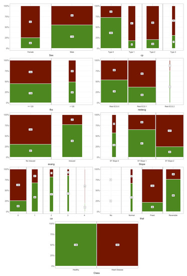
Figure 1.
Mosaic plots of categorical features.
To display the relationship between the numerical features and heart disease, the density function is represented by differentiating the values according to it (Figure 2).
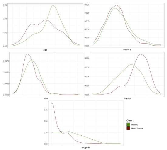
Figure 2.
Density plots of numerical features.
The plots show that there may be a correlation between age, maximum heart rate reached during the exercise test (thalach), and depression induced by exercise in relation to rest (oldpeak) with or without heart disease. These first hypotheses that could be made by visual inspection will be corroborated or refuted in the following sections where the importance of features in predicting heart disease is addressed.
3.2. Features Selection
An important point to consider is the quantity and quality of the features used. The current trend in applying machine learning techniques is to incorporate all available features. This is due to the available computing capacity and many techniques incorporating regularization mechanisms that avoid overfitting and simplify the models automatically. Reducing the independent features reduces the dimensionality, suppresses noise sources in the data that can produce biases, and improves the interpretability of the models.
There are many approaches to determining the importance of features and thus selecting features. As the goal of this work was to show the balance between the interpretability and predictive ability of the model, we will show different metrics that measure the importance of the features in order to train the classifier with different amounts of features. The accuracy and area under the ROC curve (AUC) results were compared. A total of 13 importance metrics were used based on statistical tests: ANOVA, Kruskal–Wallis test (KT), and chi-square test (Chi2); based on entropy: information gain (IG), information gain ratio (GainR), and symmetric uncertainty (SU); on measurements of models obtained with random forest: impurity (Rimp), permutation (Rper); and random forest importance (Rfi); based on decision tree models: one rule (OneR), conditional variable importance (PCF), and the importance given by the relief algorithm (Rel). All these measures were obtained with the implementation in the mlr library of R [39].
Table 2 shows the ranking value for each measure. The features are ordered by mean value (mean) of all their positions. The final value (rank) represents the order according to the mean. The proportional value between the features was not considered—only the position in the ranking is used to facilitate comparison.
Table 2.
Importance metrics.
Table 2 shows that the features for most of the metrics are in similar positions; only the Relief measure changes the positions of the features. The rank value was used to group the features into tertiles. That is, accuracy and AUC were measured using decision trees with all features, then with those in the first and second tertile, and finally only with those in the first third. This allowed us to compare the loss in accuracy versus the gain in interpretability using different amounts of features.
3.3. Performance Evaluation Methods
To measure the balance between performance and interpretability, the set of classification techniques was compared using a different number of features. A total of 100 runs were carried out for each classifier. Each run was a 4-fold cross-validation process that measured the average performance of the algorithms when they had all the features. Then, each was run with 66% of the best features (cp, thal, ca, oldpeak, thalach, exang, slope, and sex) according to the rank value in Table 2 and finally with 33% of the best features (cp, thal, ca, and oldpeak). The performance of the algorithms was compared when different amounts of attributes were used. Figure 3 shows a diagram of the process. Remember that we were not looking for the best classifier, we wanted to compare the effect of using different amounts of features on the accuracy and interpretability of the models.
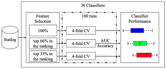
Figure 3.
Diagram of the training and testing process.
Figure 4 and Figure 5 are shown boxplots: in blue and labeled as 100 the results when all features were used, in green when 66% and red when 33% of the most important features were used. Accuracy and AUC were selected as quality measures. We compared 36 classifiers, most of which were implementations of the R caret library [40] and a few belong to the RWeka library [41]. In the final list of acronyms, we distinguish the implementations of each of the algorithms; if not specified, they correspond to the caret library.
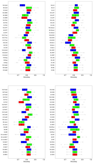
Figure 4.
Comparison of classifier performance (accuracy). Blue, all features; green, best 66% of features; red, best 33% of features.
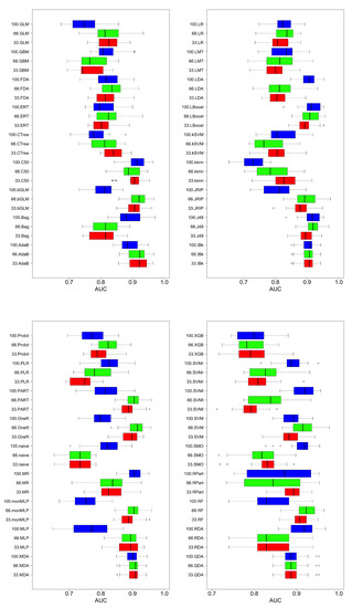
Figure 5.
Comparison of classifier performance (AUC). Blue, all features; green, best 66% of features; red, best 33% of features.
Regardless of the measure of quality, accuracy, or AUC metrics, in general, better results were obtained when using more features, although there were exceptions. For example, for discriminant analysis techniques (LDA—linear discriminant analysis—and FDA—Factorial Discriminant Analysis) or SVM, better results were obtained with fewer features than using all of them; this may be due to the characteristics of the classification algorithms. They tried to partition the classification space using hyperplanes to make the decision. With more features, without a mechanism that can filter or weigh them, it introduced noise when performing the partitioning of the classification space. There are algorithms that can perform progressive refinements of the model until the limit where overfitting occurs. Examples of this type are those that use boosting or bagging (Random Forest is characteristic of this behavior), where using more features produces better results because the model can be adjusted in a more complex way: the decision space is subdivided into hyper-rectangles. The disadvantage of these techniques is that they produce better results at the cost of increased difficulty of interpreting the model that guides its decisions. The decision trees are in an intermediate position: they do not produce the performance of the boosting techniques but they improve the classifiers based on hyperplane partitions, maintaining a high understanding of their models. This is why they are used in the following discussion of the behavior of complexity versus the quality of the solution.
To visualize the effect of the number of features on the complexity of the results and their associated quality, we examined how AUC varied according to the depth of the tree. The AUC results of trees obtained with RPART [37] and Ctree [38] were reported. A total of 100 executions of the algorithms were performed using hold-out (70–30%) representing the mean value and the confidence interval at 95% of the AUC over the test set in Figure 6.
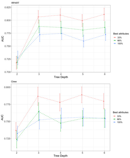
Figure 6.
Variation in the performance (AUC) with the tree depth and the percentage of features used. Up, recursive partitioning and regression trees (RPART); Down, conditional inference trees (Ctree).
RPART is an R implementation of the classification and regression trees (CART) algorithm. The algorithm is well-known and applied in two stages. In the first step, the data are divided by rules using the attribute that best separates the data according to the values of the target attribute. This process continues until the data are completely split. It uses the GINI index as a splitting criterion. The rules can be expressed in the form of a tree, which is the most common method to represent the result obtained by RPART. In the second stage, to avoid overfitting, the algorithm performs a pruning of the tree considering a complexity regularization factor. RPART has some known limitations, such as attribute selection being biased to allow more cutpoints [42]. This means that attributes with a larger value range or more categories are selected. Ctree is a decision tree creation algorithm that does not have this drawback. It is based on a statistical inference framework and selects the attributes by applying a statistical test to select the best attribute with which to split the data.
Both algorithms behaved similarly, like linear partitioning algorithms: adding features did not improve the quality of the solutions. The curve corresponding to the use of all features always appeared below the curves with fewer features. The one with the highest value was the one with the least number of features. If relevant features in the nodes were chosen poorly, then the mistake was propagated to the decision of the class. This finding supports the importance of correctly choosing features to be used when solving a classification task.
The behavior with the depth level of the best classification tree was expected. As the depth of the tree increased, i.e., its complexity, its behavior improved. The level of complexity was inversely associated with the ability to interpret the model: the more complex the model, the less interpretable. In Figure 6 when the depth of the tree increased, the AUC grew to a maximum level; although the complexity continued growing, it no longer improved the performance. An interesting result was the Pareto front structure that appeared between complexity and performance, regardless of the number of features used. If it is assumed that complexity makes the classification model less interpretable, then a design decision must always be made between them. In this case, for the problem of classifying cardiovascular diseases, the price was small and the saturation of complexity occurred when a depth of three was reached. For problems with many more instances, a Pareto front with a smoother curve with depth saturation was to be expected. Depending on the problem and the technique, the curves corresponding to the amount of features were reversed. In Figure 7, Figure 8 and Figure 9, the variation in AUC was 0.06 for RPART when increasing the tree depth from two to three, and had a lower value, approximately 0.05 for Ctree. The expert analyst must determine if they want to have a more precise or more interpretable model. This is a design decision similar to finding the elbow point in a clustering problem in which precision must be balanced with the number of clusters obtained. The figure below shows the trees’ best accuracy corresponding to RPART with different numbers of features for a maximum depth of six.
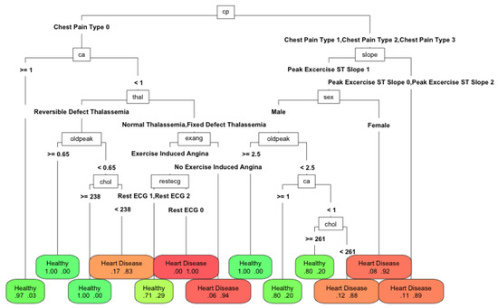
Figure 7.
Performance of RPART with 100% of features with a maximum tree depth of 6.
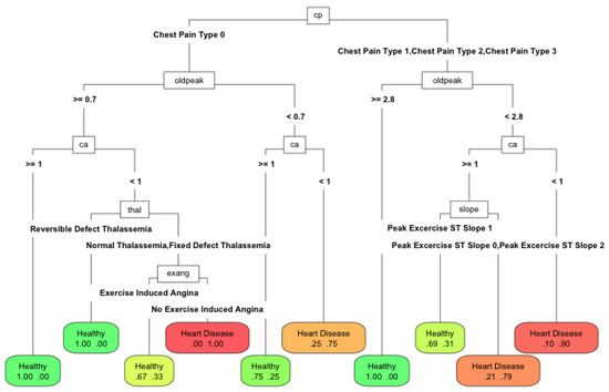
Figure 8.
Performance of RPART using 66% of features with a maximum tree depth of 6.
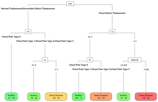
Figure 9.
Performance of RPART using 33% of features with a maximum tree depth of 6.
The differences between the methods were minimal: in accuracy, it was about 0.07. With 100% and 66% of the features, the depth of the tree increased (25 and 19 nodes and nine and six features, respectively). The algorithm tries to exploit all the available information. However, with 33% of the best features (13 nodes and four features), the depth reduced, since it could no longer use the available features to improve the solution. Therefore, it was more appropriate to reduce the number of available features. In this case, the number of features was a proxy variable for maximum depth and therefore the complexity. The Pareto front obtained using the depth was similar to that which would be obtained by modifying the amount of available features. Therefore, the compromise was the number of features used to make a model explainable. In this work, we wanted to highlight the importance of the choice of features to perform machine learning tasks. Their number will determine the quality of the solution and the ease of interpretation of the obtained models. This is an issue that is currently being neglected in the era of big data. The computational capacity has grown so much that the algorithms are applied without meticulously reducing the input features. However, the need to make the algorithm’s decisions more interpretable has become another factor to consider when applying automatic learning techniques. This paper demonstrated the relationship between interpretability and the features used and how it is an additional factor for data scientists to consider.
4. Conclusions
In this work, the multi-objective nature of the problem of improving the accuracy of classification versus the interpretability of the obtained model was analysed. We proposed a methodology composed of several steps: ranking of features, selecting the set of features for a prediction problem, testing using several ML techniques, and, finally, deciding how many features are needed to be used in a rule system to produce similar performance to any other ML technique. This methodology is based in two ideas: selecting few features and using a rule system to generate predictive explainable systems (if the performance is similar to other techniques). We showed how to develop these ideas in a real problem using the Statlog data set, following the steps of a data analysis process. First, the most relevant features were characterized, applying a ranking that incorporates the importance of these features according to different metrics. Then, different classification algorithms were compared by applying different quality metrics with different numbers of features. For most techniques, as expected, we found that better results are obtained using a larger number of features. Classification algorithms based on rules and trees behave similarly, but somewhat worse than algorithms that use a boosting processes. However, they provide a simple explanation of the underlying model. Finally, we showed that for two tree-based algorithms, the reduction in the number of input features not only improves the interpretability of the results but also improves the quality of the solutions, although a compromise is required between the complexity that can be achieved with the features and the accuracy of the classification obtained. These results are promising and, in future work, are expected to be applied to other, more comprehensive data sets of a different nature.
Author Contributions
Conceptualization, M.A.P., A.B., and J.M.M.; Formal analysis, A.B. and R.P.; Software, A.B. and R.P.; Supervision, J.M.M. and M.A.P.; Writing—original draft, R.P., A.B., M.A.P. and J.M.M.; Writing—review and editing, R.P., A.B., M.A.P. and J.M.M. All authors have read and agreed to the published version of the manuscript.
Funding
This work was funded by public research projects of Spanish Ministry of Economy and Competitivity (MINECO) (MINECO), references TEC2017-88048-C2-2-R, RTC-2016-5595-2, RTC-2016-5191-8, and RTC-2016-5059-8.
Conflicts of Interest
The funders had no role in the design of the study; in the collection, analyses, or interpretation of data; in the writing of the manuscript, or in the decision to publish the results.
Abbreviations
The following abbreviations are used in this manuscript:
| AdaB | AdaBoost classification trees |
| AUC | Area under the ROC curve |
| Bag | Bagging (Weka implementation) |
| bGLM | Boosting for generalized linear models |
| C50 | C5.0 classification trees |
| CAD | Coronary artery disease |
| CART | Classification and regression trees |
| Chi2 | Chi-square test |
| Ctree | Conditional inference trees |
| EMLA | Ensemble machine learning algorithm |
| ERT | Extremely randomized trees |
| FDA | Flexible discriminant analysis |
| GainR | Information gain ratio |
| GBM | Gradient boosting machine |
| GLM | Generalized linear models |
| IG | Information gain |
| J48 | C4.5 Classification trees |
| JRIP | Propositional rule learner |
| kknn | k-nearest neighbours (caret implementation) |
| kSVM | Kernel support vector machine |
| KT | Kruskal–Wallis test |
| IBk | k-nearest neighbours (Weka implementation) |
| LBoost | Boosted logistic regression |
| LDA | Linear discriminant analysis |
| LMT | Logistic model trees |
| LR | Logistic regression |
| naive | Naïve Bayes |
| MDA | Mixture discriminant analysis |
| MLP | Multi-layer perceptron |
| monMLP | Monotone multi-layer perceptron |
| MR | Multinomial regression |
| OneR | 1-R classifier |
| PART | PART decision lists |
| PCF | Conditional variable importance |
| PLR | Logistic regression with a L2 penalty |
| Probit | Probit regression |
| QDA | Quadratic discriminant analysis |
| RDA | Regularized discriminant analysis |
| Rel | Relief |
| RF | Random forest |
| RFi | Random forest importance |
| Rimp | Impurity importance |
| RPART | Recursive partitioning and regression trees |
| Rper | Permutation importance |
| SMO | Support vector machine (Weka implementation) |
| SU | Symmetric uncertainty |
| SVM | Support vector machine (caret implementation) |
| SVMr | Regression support vector machine |
| SVMl | Least squares support vector machine |
| XGB | Extreme gradient boosting |
References
- Carvalho, D.V.; Pereira, E.M.; Cardoso, J.S. Machine learning interpretability: A survey on methods and metrics. Electronics 2019, 8, 832. [Google Scholar] [CrossRef]
- World Health Organization. Fact Sheet: Cardiovascular Diseases (CVDs); World Health Organization: Geneva, Switzerland, 2017. [Google Scholar]
- Fagard, R.H. Predicting risk of fatal cardiovascular disease and sudden death in hypertension. J. Hypertens. 2017, 35, 2165–2167. [Google Scholar] [CrossRef]
- King, R.D.; Feng, C.; Sutherland, A. Statlog: Comparison of classification algorithms on large real-world problems. Appl. Artif. Intell. 1995, 9. [Google Scholar] [CrossRef]
- Ansari, M.F.; AlankarKaur, B.; Kaur, H. A prediction of heart disease using machine learning algorithms. Adv. Intell. Syst. Comput. 2021, 1200. [Google Scholar] [CrossRef]
- Turki, T.; Wei, Z. Boosting support vector machines for cancer discrimination tasks. Comput. Biol. Med. 2018, 101. [Google Scholar] [CrossRef] [PubMed]
- Nilashi, M.; Bin Ibrahim, O.; Mardani, A.; Ahani, A.; Jusoh, A. A soft computing approach for diabetes disease classification. Health Inform. J. 2018, 24. [Google Scholar] [CrossRef] [PubMed]
- Leslie, H.H.; Zhou, X.; Spiegelman, D.; Kruk, M.E. Health system measurement: Harnessing machine learning to advance global health. PLoS ONE 2018, 13, e0204958. [Google Scholar] [CrossRef]
- Almustafa, K.M. Prediction of heart disease and classifiers’ sensitivity analysis. BMC Bioinform. 2020, 21. [Google Scholar] [CrossRef]
- Fatima, M.; Pasha, M. Survey of Machine Learning Algorithms for Disease Diagnostic. J. Intell. Learn. Syst. Appl. 2017, 9. [Google Scholar] [CrossRef]
- El Houby, E.M. A survey on applying machine learning techniques for management of diseases. J. Appl. Biomed. 2018, 16, 165–174. [Google Scholar] [CrossRef]
- Bahadur, S. Predict the Diagnosis of Heart Disease Patients Using Classification Mining Techniques. IOSR J. Agric. Vet. Sci. 2013, 4, 60–64. [Google Scholar] [CrossRef]
- Liu, X.; Wang, X.; Su, Q.; Zhang, M.; Zhu, Y.; Wang, Q.; Wang, Q. A Hybrid Classification System for Heart Disease Diagnosis Based on the RFRS Method. Comput. Math. Methods Med. 2017, 2017. [Google Scholar] [CrossRef] [PubMed]
- Digital Single Market. Draft Ethics Guidelines for Trustworthy AI | Digital Single Market. 2019. Available online: https://ec.europa.eu/digital-single-market/en/news/ethics-guidelines-trustworthy-ai. (accessed on 15 December 2020).
- Zhang, Z.; Xie, Y.; Xing, F.; McGough, M.; Yang, L. MDNet: A semantically and visually interpretable medical image diagnosis network. In Proceedings of the 30th IEEE Conference on Computer Vision and Pattern Recognition, CVPR 2017, Seattle, WA, USA, 21–23 June 2017. [Google Scholar] [CrossRef]
- Hicks, S.A.; Eskeland, S.; Lux, M.; Lange, T.D.; Randel, K.R.; Pogorelov, K.; Jeppsson, M.; Riegler, M.; Halvorsen, P. Mimir: An automatic reporting and reasoning system for deep learning based analysis in the medical domain. In Proceedings of the 9th ACM Multimedia Systems Conference, MMSys 2018, Amsterdam, The Netherlands, 12–15 June 2018. [Google Scholar] [CrossRef]
- Choi, E.; Bahadori, M.T.; Kulas, J.A.; Schuetz, A.; Stewart, W.F.; Sun, J. RETAIN: An interpretable predictive model for healthcare using reverse time attention mechanism. arXiv 2016, arXiv:1608.05745. [Google Scholar]
- Ma, F.; Chitta, R.; Zhou, J.; You, Q.; Sun, T.; Gao, J. Dipole: Diagnosis prediction in healthcare via attention-based bidirectional recurrent neural networks. In Proceedings of the ACM SIGKDD International Conference on Knowledge Discovery and Data Mining, Halifax, NS, Canada, 13–17 August 2017. [Google Scholar] [CrossRef]
- Sha, Y.; Wang, M.D. Interpretable predictions of clinical outcomes with an attention-based recurrent neural network. In Proceedings of the 8th ACM International Conference on Bioinformatics, Computational Biology, and Health Informatics, Boston, MA, USA, 20–23 August 2017. [Google Scholar] [CrossRef]
- Rögnvaldsson, T.; Etchells, T.A.; You, L.; Garwicz, D.; Jarman, I.; Lisboa, P.J. How to find simple and accurate rules for viral protease cleavage specificities. BMC Bioinform. 2009, 10. [Google Scholar] [CrossRef]
- Che, Z.; Purushotham, S.; Khemani, R.; Liu, Y. Interpretable Deep Models for ICU Outcome Prediction. AMIA Annu. Symp. Proc. 2016, 2016, 371. [Google Scholar]
- Wu, M.; Hughes, M.C.; Parbhoo, S.; Zazzi, M.; Roth, V.; Doshi-Velez, F. Beyond sparsity: Tree regularization of deep models for interpretability. In Proceedings of the 32nd AAAI Conference on Artificial Intelligence, AAAI 2018, New Orleans, LA, USA, 2–7 February 2018. [Google Scholar]
- Dua, D.; Graff, C. UCI Machine Learning Repository. 2017. Available online: https://archive.ics.uci.edu/ml/index.php (accessed on 29 September 2020).
- Abdar, M.; Kalhori, S.R.; Sutikno, T.; Subroto, I.M.I.; Arji, G. Comparing performance of data mining algorithms in prediction heart diseses. Int. J. Electr. Comput. Eng. 2015, 5. [Google Scholar] [CrossRef]
- El-Bialy, R.; Salamay, M.A.; Karam, O.H.; Khalifa, M.E. Feature Analysis of Coronary Artery Heart Disease Data Sets. Procedia Comput. Sci. 2015, 65. [Google Scholar] [CrossRef]
- Naushad, S.M.; Hussain, T.; Indumathi, B.; Samreen, K.; Alrokayan, S.A.; Kutala, V.K. Machine learning algorithm-based risk prediction model of coronary artery disease. Mol. Biol. Rep. 2018, 45. [Google Scholar] [CrossRef]
- Chaurasia, V.; Pal, S. Data Mining Approach to Detect Heart Diseases. Int. J. Adv. Comput. Sci. Inf. Technol. 2013, 2, 56–66. [Google Scholar]
- Dhayanand, S.; Vijayarani1, M. Liver Disease Prediction using SVM and Naïve Bayes Algorithms. Int. J. Sci. Eng. Technol. Res. 2015, 4, 816–820. [Google Scholar]
- Zhao, Y.; Healy, B.C.; Rotstein, D.; Guttmann, C.R.; Bakshi, R.; Weiner, H.L.; Brodley, C.E.; Chitnis, T. Exploration of machine learning techniques in predicting multiple sclerosis disease course. PLoS ONE 2017, 12, e0174866. [Google Scholar] [CrossRef] [PubMed]
- Samuel, O.W.; Asogbon, G.M.; Sangaiah, A.K.; Fang, P.; Li, G. An integrated decision support system based on ANN and Fuzzy_AHP for heart failure risk prediction. Expert Syst. Appl. 2017, 68. [Google Scholar] [CrossRef]
- Jin, B.; Che, C.; Liu, Z.; Zhang, S.; Yin, X.; Wei, X. Predicting the Risk of Heart Failure with EHR Sequential Data Modeling. IEEE Access 2018, 6. [Google Scholar] [CrossRef]
- Long, N.C.; Meesad, P.; Unger, H. A highly accurate firefly based algorithm for heart disease prediction. Expert Syst. Appl. 2015, 42. [Google Scholar] [CrossRef]
- Pawar, U.; O’Shea, D.; Rea, S.; O’Reilly, R. Explainable AI in Healthcare. In Proceedings of the 2020 International Conference on Cyber Situational Awareness, Data Analytics and Assessment, Dublin, Ireland, 15–19 June 2020. [Google Scholar] [CrossRef]
- Ahmad, M.A.; Teredesai, A.; Eckert, C. Interpretable machine learning in healthcare. In Proceedings of the 2018 IEEE International Conference on Healthcare Informatics, ICHI 2018, New York, NY, USA, 4–7 June 2018. [Google Scholar] [CrossRef]
- Rudin, C. Please Stop Explaining Black Box Models for High Stakes Decisions. arXiv 2018, arXiv:1811.10154. [Google Scholar]
- Towards Trustable Machine Learning. 2018. Available online: https://doi.org/10.1038/s41551-018-0315-x (accessed on 21 November 2020).
- Breiman, L.; Friedman, J.H.; Olshen, R.A.; Stone, C.J. Classification and Regression Trees; Chapman and Hall/CRC: London, UK, 2017. [Google Scholar] [CrossRef]
- Hothorn, T.; Hornik, K.; Zeileis, A. Unbiased recursive partitioning: A conditional inference framework. J. Comput. Graph. Stat. 2006, 15. [Google Scholar] [CrossRef]
- Bischl, B.; Lang, M.; Kotthoff, L.; Schiffner, J.; Richter, J.; Studerus, E.; Casalicchio, G.; Jones, Z.M. Mlr: Machine learning in R. J. Mach. Learn. Res. 2016, 17, 5938–5942. [Google Scholar]
- Max, K. Building Predictive Models in R Using the caret Package. J. Stat. Softw. 2008, 28, 1–26. [Google Scholar]
- Hornik, K.; Buchta, C.; Zeileis, A. Open-source machine learning: R meets Weka. Comput. Stat. 2009, 24. [Google Scholar] [CrossRef]
- Loh, W.Y. Fifty years of classification and regression trees. Int. Stat. Rev. 2014, 82. [Google Scholar] [CrossRef]
Publisher’s Note: MDPI stays neutral with regard to jurisdictional claims in published maps and institutional affiliations. |
© 2021 by the authors. Licensee MDPI, Basel, Switzerland. This article is an open access article distributed under the terms and conditions of the Creative Commons Attribution (CC BY) license (http://creativecommons.org/licenses/by/4.0/).