Article

The Lie Algebraic Approach for Determining Pricing for Trade Account Options

1
Department of Industrial Management, National Taiwan University of Science and Technology, 43 Sec. 4 Keelung Road, Daan District, Taipei 106335, Taiwan
2
Institute of Industrial Management, National Central University, 300 Zhongda Road, Zhongli District, Taoyuan City 32001, Taiwan
3
Minastir Asset Management AB, Quantitative Developer, Gottakrav. 28, 236 41 Hollviken, Sweden
*
Author to whom correspondence should be addressed.
Mathematics 2021, 9(3), 279; https://doi.org/10.3390/math9030279
Submission received: 8 January 2021 / Revised: 27 January 2021 / Accepted: 28 January 2021 / Published: 30 January 2021
(This article belongs to the Special Issue Mathematical and Statistical Methods Applications in Finance)

Abstract

:
In recent years, many advanced techniques have been applied to financial problems; however, very few scholars have used the Lie theory. The purpose of this study was to examine the options for a trade account through Lie symmetry analysis. According to our results, it is effective for determining analytical solutions for pricing issues and solving other partial differential equations. The proposed solution can be used by further researchers or practitioners in option pricing problems for better performance compared with the classical Black–Scholes model.

1. Introduction

Both researchers and practitioners have studied option pricing for over a century [1,2,3]. Many theoretical models have been proposed to help investors decide how to buy and sell an asset within a specified period [1,2,4,5,6,7], such as option pricing, which is affected by financial aspects including stock prices, interest rates and exchange rates [8]. In particular, Black and Scholes [4] presented a general equilibrium of option pricing utilizing stochastic differential equations. Their model assumes that a price dynamic follows a continuous timeline, the short-term interest rate is known and constant and the stock returns are log-normal. Merton [1] extended the Black–Scholes model to analyze rational option pricing and Cox, Ross and Rubinstein [5] examined this process utilizing arbitrage methods in a simple discrete timeline. Later, Hyer, Lipton-Lifschitz and Pugachevsky [6] introduced the passport option based on the partial differential equation (PDE) method and solved it by using the Hamilton–Jacobi–Bellman (HJB) equation. Their model was later extended by [9], who utilized both continuous and discrete switching. In addition, Shreve and Večeř [2] developed a model, which can be used for both discrete and continuous partial differential equations to ascertain general analytic solutions and determine the most effective options for a trade account (OTA).
In general, the most effective strategy regarding option pricing can be found by solving a PDE using the Lie symmetry theory. Although it has been widely adopted in physics and engineering, Gazizov and Ibragimov [10] were one of the first to apply it to the field of finance and transform the Black–Scholes equation into a classical heat equation. Later, Guillaume [11] extended this transformation into an n-dimensional equation ideal for analyzing multi-asset options. First, Taylor and Glasgow [12] established a general Lie symmetry analysis of a simple Asian option with arbitrary constants. Caister et al. [13] expanded this work by determining a more systematic and analytic version of the Asian option, which they demonstrated to be much easier than the Laplace transformation approach [14]. In a recent paper, Sinkala [15] applied Lie symmetry analysis to invariant solutions of arbitrage-free stock prices. Furthermore, Jagannathan [16] applied the diffusion process model to investigate the option pricing with three factors of the exchange rate as stochastic volatility, domestic interest rate, and return process. In addition, Paliathanasis et al. [17] investigated the stochastic volatility of European options. They argued that if the volatility function and option pricing are based on the second Brownian motion, the evolution PDEs will not be reduced to the Black–Scholes–Merton equation.
To the best of our knowledge, there is a lack of research on the Lie theory approach with regard to pricing options for trade accounts. Similarly, Vecer, Kampen and Navratil [3] derived the passport options for options on a traded account with symmetry analysis under two underlying assets. Their optimal solution is effective for option pricing of the portfolios with largest volatility, but the passport options have not been popular like European options. In this study, the European options for a traded account are examined with the Lie theory approach. Thus, the purpose of this study was to utilize this technique to achieve this goal. This paper is organized as follows: Section 2 describes the symmetry reduction method and how to group invariant solution intuitively. Section 3 presents the best options for a trade account. Section 4 illustrates how to utilize symmetry analysis to determine the most effective options in this context. The conclusion and recommendations for future studies are found in Section 5.

2. Symmetry Analysis

Symmetry analysis is one of the most powerful analytical techniques for systematically solving PDEs through transformation. According to Lie [18], differential equations can be integrated or reduced to lower-order terms based on synthesis symmetry. Specifically, Baumann [19] found that two independent variables x , t , and one dependent variable v can be solved using the equation below:
Δ ( v , x , t , v x , v t , 2 v x 2 , 2 v t 2 , 2 v x t ) = 0
which illustrates one parameter of the Lie group of transformations.
x ˜ = T x ( x , t , v ; ϵ ) t ˜ = T t ( x , t , v ; ϵ ) v ˜ =   T v ( x , t , v ; ϵ )
If we assume the solution to Equation (1) is v =   θ ( x , t ) , the transformations can be expressed as follows:
x ˜ = T x ( x , t , θ ( x , t ) ; ϵ ) t ˜ = T t ( x , t , θ ( x , t ) ; ϵ ) v ˜ = T v ( x , t , θ ( x , t ) ; ϵ )
Therefore, v ˜ is the solution to the transformations. This unique problem can be solved by using the functional equation:
θ = ( T x ( x , t , θ ( x , t ) ; ϵ ) ,   T t ( x , t , θ ( x , t ) ; ϵ ) ) = v ˜
By replacing the transformations in Equation (3) with infinitesimal representations, we obtain the following new equations:
x ˜ = x + ϵ ξ 1 ( x , t , v ; ϵ ) t ˜ = t + ϵ ξ 2 ( x , t , v ; ϵ ) v ˜ = v + ϵ 1 ( x , t , v ; ϵ )
Then, Equation (4) can be simplified with the infinitesimal representations with ϵ as the group parameter shown below:
θ + ϵ 1 ( x , t , θ ; ϵ ) = θ ( x + ϵ ξ 1 ( x , t , θ ; ϵ ) , t + ϵ ξ 2 ( x , t , θ ; ϵ ) )  
According to the Taylor expansion, we can subtract the left-hand side from the right-hand side of Equation (6) to yield ϵ = 0 as shown:
ξ 1 θ x + ξ 2 θ t 1 = 0
Thus, the invariant surface condition of the first-order PDE can be determined as follows:
v · F ( x , t , v ) = ξ 1 F x + ξ 2 F t 1 F v = 0
where the tangent vector v is calculated in the equation as shown:
v = ξ 1 x + ξ 2 t + 1 v
We can solve the invariant condition of first-order PDEs with the unit vectors ξ 1 , ξ 2 , and 1 by using the following characteristics of differential equations:
d x ˜ d ϵ = ξ 1 ( x ˜ , t ˜ , v ˜ ) d t ˜ d ϵ = ξ 2 ( x ˜ , t ˜ , v ˜ ) d v ˜ d ϵ = 1 ( x ˜ , t ˜ , v ˜ )
where the initial conditions are as follows:
d x ˜ d ϵ | = 0 = x ,   d t ˜ d ϵ | = 0 = t ,   d v ˜ d ϵ | = 0 = v
After reducing Equation (1), the PDEs can be solved analytically via the characteristic curves. Further analysis of the characteristic differential equations can be found in [20].

3. Options for a Trade Account

This allows the holder to switch among their trade portfolios, such as stocks [2,3], when the equity accumulation is equal to profit/loss values during the entire trading period. In the early studies of options for trade accounts, Shreve and Večeř [2] explored vacation call and put options with regard to the boundaries of the strategy holder. They argued that these elements provide more possibilities than traditional call and put in the American stock market. In this study, we employed the risk-neutral measure of stock price S t in the stochastic differential equation below:
d S t S t = r d t + σ d W t
where r, σ, and W t are the interest rate, the volatility of the stock and a one-dimensional standard Brownian motion. According to [2], the option holder strategy can be expressed in the following equation:
d X t q = q t d S t + μ ( X t q   q t S t ) d t
The option holder’s trading strategy with the number of shares held at time t is q t , while he or she might hold either α t or β t shares at any given time for q t [ α t ,   β t ] and α t β t . The goal of the option holder, to a maximum of the expected value of all possible strategies q u , can be achieved using the equation shown below:
V [ α , β ] ( t , S t , X t ) =   max q u [ α , β ] e r ( T t ) E [ ( X T q ) + | F t , ]   for   t [ 0 , T ]
where X T q is the payoff to the holder at time T . The objective function V [ α , β ] ( t , S t , X t ) can be displayed in the Hamilton–Jacobi–Bellman (HJB) equation to determine the boundary condition V ( T , s , x ) = x + as:
V t + r s V s r V + max q [ α , β ] [ ( μ x + q ( r μ ) ) V x + 1 2 σ 2 s 2 ( V s s + 2 q V s x + q 2 V x x ) ] = 0
By changing the variable Z t q = X t q S t , we can reduce the dimensionality of Equation (13) and correspondingly reduce the HJB equation with the boundary condition u ( T , z ) = z + as follows:
u t + max q [ α , β ] [ ( r μ ) ( q z ) u z + 1 2 σ 2 ( q z ) 2 u z z ] = 0
The relationship between V and u is shown as:
V ( t , s , x ) = s · u ( t , x s )
The option holder can prioritize in the case of European options when α t = β t . If both shares are equal to 1, the problem is reduced to the European call. However, it can be reduced to the European put when α t = β t = 1 . In the passport option, when α t = 0 and β t = 1 , the problem can be expressed as a vacation call and a put if α t = 1 and β t = 0 .

4. Utilizing Symmetry Analysis for the Pricing Problem

In this section, we apply symmetry analysis to determine the optimal strategy with regard to the pricing problem. We utilize the HJB Equation (16) to obtain the European option equation shown below:
u t + ( r   μ ) ( q z ) u z +   1 2 σ 2 ( q z ) 2 u z z = 0
Following the prolongation formula discussed by Olver [21], we can obtain the characteristic differentials associated with Equation (18), which is written as follows:
4 ξ 1   ( q z ) ( 4 ( ξ 1 ) z + 2 ( ξ 2 ) t + ( q z ) ( 2 ( r   μ ) ( ξ 2 ) z + ( q z ) σ 2 ( ξ 2 ) z z ) ) = 0
( q z ) ( 2 ( r   μ ) ( ξ 1 ) z + 2 ( r   μ ) ( ξ 2 ) t + ( q z ) ( 2 ( r   μ ) 2 ( ξ 2 ) z )                                                               σ 2 ( ( ξ 1 ) z z ( q z ) ( r   μ ) ( ξ 2 ) z z ) 2 ( 1 ) z u ) ) )                                                             2 ( ( r   μ ) ξ 1 + ( ξ 1 ) t ) =   0
2 ( 1 ) t + ( q z ) ( 2 ( r   μ ) ( 1 ) z + ( q z ) 2 σ 2 ( 1 ) z z ) =   0
2 ( ξ 1 ) u ( q z ) 2 σ 2 ( ξ 2 ) z u = 0
2 ( ξ 1 ) z u 2 ( r μ ) ( q z ) ( ξ 2 ) z u ( 1 ) u u = 0
( ξ 1 ) u u ( r   μ ) ( q z ) ( ξ 2 ) u u = 0
( ξ 2 ) z = ( ξ 2 ) u u = ( ξ 2 ) u = 0
The solutions are illustrated in the equations below:
ξ 1 =   1 4 ( ( q z ) ( 4 a 4 + 2 a 2 t ( r   μ ) + ( a 2 4 a 5 ) t σ 2 )                                                                 + 2 ( z q ) ( a 2 + 16 a 3 t σ 2 ( 2 r 2 μ +   σ 2 ) 2 ln ( z   q ) )
ξ 2 =   a 1 + t ( a 2 +   8 a 3 t σ 2 ( 2 r 2 μ +   σ 2 ) 2 )
1 = u ( a 6 +   a 3 t 2 + a 5 ln ( z q ) +   4 a 3 ( ln ( z q ) ) 2 ( 2 r 2 μ +   σ 2 ) 2 + t 8 a 3 σ 2 + ( 2 r 2 μ +   σ 2 ) ( a 5 ( 2 r 2 μ +   σ 2 ) 2 + 8 a 3 ln ( z q ) ) 2 ( 2 r 2 μ +   σ 2 ) 2 )
where a i for i from 1–6 become the arbitrary constants. They also provide the infinite-dimensional vector space for the infinitesimal symmetries of Equation (18), including the following operators:
V 1 =   t
V 2 = t t +   k 2 z +   k 3 z z +   k 4 ln ( z q ) z +   k 5 ln ( z q ) z z
V 3 =   1 k 1 ( k 6 t 2 t +   k 7 u u + k 8 ln ( z q ) z + k 9 ln ( z q ) z z )
V 4 =   k 10 z
V 5 =   k 11 u u +   k 12 z +   k 13 z z
V 6 = u u
where k i for i from 1–6 are defined by r, μ, σ, q, t. Also, the symmetry algebra is calculated using Equations (29)–(34) to establish an invariant solution for Equation (18). If v = F ( η ,   t ) , in this scenario, we have:
v =   1 ( x ,   t ,   v ;   ϵ ) | ϵ 0
By assuming the value of a 1 a 6 and c 1 and c 2 ( a 2 =   a 3 =   a 5 = 0 ,   a 1 =   c 1 ,   a 4 =   c 2   and   a 6 = 1 ) , Equations (26)–(28) can be determined.
ξ 1 =   c 2 ( q z ) ,         ξ 2 =   c 1 ,         1 = u
After finding the relationship between variables z and t, the invariant under the symmetry group of Equations (29)–(34) can be calculated using the following equation:
i n v =   c 2 t c 1 ln ( q z )   for   c 1 ,   c 2     0
Because of ζ = t   c 1 c 2 ln ( q z ) and the group invariant solution of the PDE (18), we have:
σ 2   c 2 ( 2 ( r   μ ) +   σ 2 ) ) F ( ζ ) + ( 2 c 2 ( c 2 +   c 1 ( r μ ) ) + ( 2 c 2 ( c 2 +   c 1 ( r u ) ) +   c 1 ( c 2 2 ) σ 2 ) F ( ζ ) +   c 1 2 σ 2 F ( ζ ) = 0
where
F ( ζ ) = ( q z ) 1 c 2 u ( z , t )
The F ( ζ ) is the function with the arbitrary constants w 1 and w 2 :
F ( ζ ) =   w 1 e g 1 ζ + w 2 e g 2 ζ
where
g 1 = 2 c 2 ( c 2 + c 1 ( r μ ) ) +   c 1 ( c 2 2 ) σ 2 2 c 1 2 σ 2 + c 2 2 ( 4 ( c 2 + c 1 ( r μ ) ) 2 + 4 c 1 ( c 2 2 + c 1 ( r μ ) σ 2 +   c 1 2 σ 4 ) ) 2 c 1 2 σ 2
g 2 = 2 c 2 ( c 2 + c 1 ( r μ ) ) +   c 1 ( c 2 2 ) σ 2 2 c 1 2 σ 2 c 2 2 ( 4 ( c 2 + c 1 ( r μ ) ) 2 + 4 c 1 ( c 2 2 + c 1 ( r μ ) σ 2 +   c 1 2 σ 4 ) ) 2 c 1 2 σ 2
The invariant solution is shown in the following equation:
u ( z , t ) = w 1 ( q z ) 1 c 1 g 1 c 2 e g 1 t + w 2 ( q z ) 1 c 1 g 2 c 2 e g 2 t
The relationship between V and u can be determined by utilizing Equation (17),
V ( s , x , t ) = w 1 s c 1 g 1 + c 2 1 c 2 ( q s x ) 1 c 1 g 1 c 2 e g 1 t + w 2 s c 1 g 2 + c 2 1 c 2 ( q s x ) 1 c 1 g 2 c 2 e g 2 t

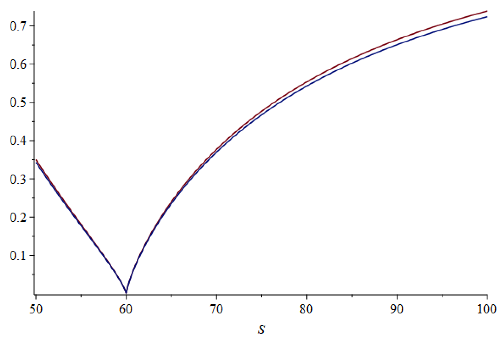
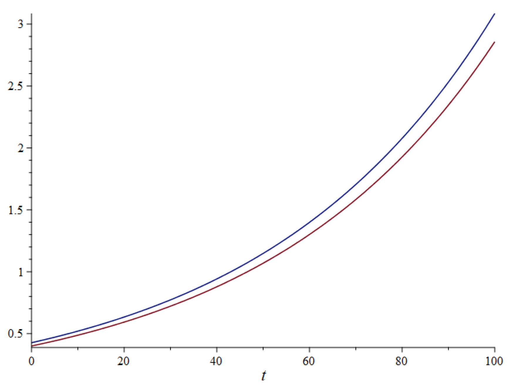
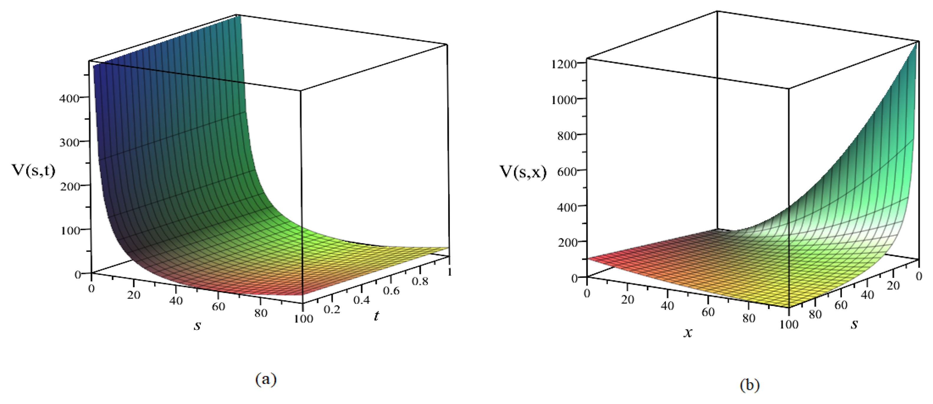
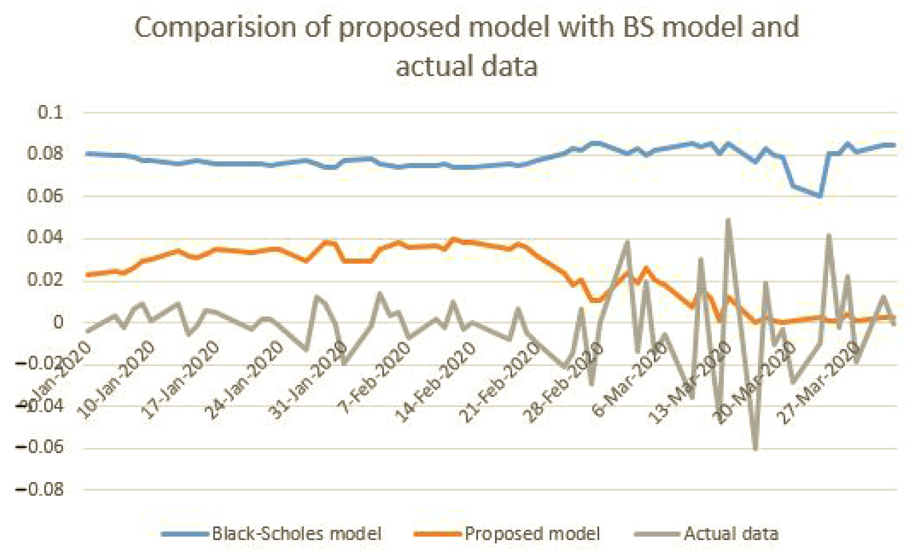
5. Numerical Example

In this section, the numerical example below is used to quantify the observed changes in option pricing due to the effect of time t and underlying asset s. Figure 1 illustrates the plotting of option pricing v(s, x, t) under time t and the underlying asset s. The following equation can be used to obtain the value of the claim parameter:
1 c 1 g 1 c 2 = 1 c 1 g 2 c 2 = 2
where r = 0.01 ,     μ = 0.005 ,     σ =   0.3 ,   T = 1 , x = 60 , q = 1 , w 1 = 1 , w 2 = 0.005 , and the values of c 1 and c 2 are determined.
According to Figure 1a, if the underlying asset is at 60, the option pricing is convex at the lowest point. The value of option pricing is linearly decreased when the time is increased from 0 to 1. Also, the two highest points of option pricing are approximately over 400 if the time and underlying asset are near 0. Figure 1b shows that the optimal solution seems to slightly decrease when we increase the value of x and s. Comparing the two plots in Figure 1, we can easily recognize that the sensitivity of strike price x is larger than time t with the underlying assets, especially when s is below 60.
In Figure 2, the dataset of the Apple stock price from 3 January 2020 to 31 March 2020 is used for comparing the performance of the proposed model with the Black–Scholes model with log returns. The proposed model line (orange color) more closely resembles the actual dataset (gray color) than the classical Black–Scholes model (blue color). Especially, when the stock price was hardly fluctuating during March 2020, the proposed model was decreasing to near zero points rather than still keeping the stable line from the Black–Scholes model, which indicates that our proposed model outperforms the Black–Scholes model of option pricing problem. Also, the sensitivity of the option price is conducted for testing the effect of stock price when t = 0 and t = 1 with underlying assets in Figure 3. Moreover, the sensitivity of the option of theta is shown in Figure 4. The difference of option sensitivity between two underlying assets s = 30 (red line) and s = 100 for (blue line) is linearly increasing t in the range of 0–100.

6. Conclusions

In this study, we utilized Lie symmetry analysis to determine pricing options for a trade account problem. Although the Lie theory requires a massive number of algebraic calculations, we have demonstrated that symmetry analysis is a powerful technique for analyzing systemic problems in the field of finance. The proposed model also shows that it outperforms the classical Black–Scholes model in the actual dataset. In the future, other techniques can be studied to find the solution of options for a trade account such as Monte Carlo simulation [22] or the jump-diffusion model [23,24]. The probabilistic approach is another effective way to find the optimal solution to the option pricing problem [25]. The real option of R&D expenditure did not garner enough attention by researchers, but the impact of R&D financial information has significant influence on the optimal solution of financial markets [26,27]. To evaluate the pricing through perceived value [28] of current stock price rather than to consider cost-related price traditionally only can reduce the gap of cost–value. Besides, sustainability, corporate governance and Corporate Social Responsibility (CSR) are among the emerging research topics, not only in marketing and industrial management, but also in finance, such as real options [29,30,31]. For sustainable finance, real CSR options and corporate governance factors should be considered for options for a trade account in further studies. Also, the sentiment factor cannot be ignored in the performance of the financial research [32].

Author Contributions

Conceptualization, S.-H.T., T.S.N. and R.-C.W.; formal analysis, S.-H.T., T.S.N. and R.-C.W.; investigation, S.-H.T., T.S.N. and R.-C.W.; methodology, S.-H.T., T.S.N. and R.-C.W.; supervision, S.-H.T. and R.-C.W.; validation, S.-H.T., T.S.N. and R.-C.W.; visualization, S.-H.T., T.S.N. and R.-C.W.; writing—original draft, T.S.N. and R.-C.W.; writing—review and editing, S.-H.T. and T.S.N. All authors have read and agreed to the published version of the manuscript.

Funding

This research received no external funding.

Institutional Review Board Statement

Not applicable.

Informed Consent Statement

Not applicable.

Data Availability Statement

Stock dataset. Available online: https://finance.yahoo.com/quote/AAPL/options/ (accessed on 20 January 2020).

Conflicts of Interest

The authors declare no conflict of interest.

References

  1. Merton, R.C. Theory of rational option pricing. Bell J. Econ. Manag. Sci. 1973, 4, 141–183. [Google Scholar] [CrossRef] [Green Version]
  2. Shreve, S.E.; Večeř, J. Options on a traded account: Vacation calls, vacation puts and passport options. Financ. Stoch. 2000, 4, 255–274. [Google Scholar] [CrossRef]
  3. Vecer, J.; Kampen, J.; Navratil, R. Options on a traded account: Symmetric treatment of the underlying assets. Quant. Financ. 2020, 20, 37–47. [Google Scholar] [CrossRef]
  4. Black, F.; Scholes, M. The pricing of options and corporate liabilities. J. Political Econ. 1973, 81, 637–654. [Google Scholar] [CrossRef] [Green Version]
  5. Cox, J.C.; Ross, S.A.; Rubinstein, M. Option pricing: A simplified approach. J. Financ. Econ. 1979, 7, 229–263. [Google Scholar] [CrossRef]
  6. Hyer, T.; Lipton-Lifschitz, A.; Pugachevsky, D. Passport to success: Unveiling a new class of options that offer principal protection to actively managed funds. Risk Lond. Risk Mag. Ltd. 1997, 10, 127–132. [Google Scholar]
  7. Vecer, J. A new PDE approach for pricing arithmetic average Asian options. J. Comput. Financ. 2001, 4, 105–113. [Google Scholar] [CrossRef] [Green Version]
  8. Malloch, H., Jr. The Valuation of Options on Traded Accounts: Continuous and Discrete Time Models. Ph.D. Thesis, University of Sydney, Sydney, Australia, 1 August 2010. [Google Scholar]
  9. Andersen, L.; Andreasen, J.; Brotherton-Ratcliffe, R. The passport option. J. Comput. Financ. 1998, 1, 15–36. [Google Scholar] [CrossRef]
  10. Gazizov, R.K.; Ibragimov, N.H. Lie symmetry analysis of differential equations in finance. Nonlinear Dyn. 1998, 17, 387–407. [Google Scholar] [CrossRef]
  11. Guillaume, T. On the multidimensional Black–Scholes partial differential equation. Ann. Oper. Res. 2019, 281, 229–251. [Google Scholar] [CrossRef]
  12. Taylor, S.; Glasgow, S. A novel reduction of the simple Asian option and Lie-group invariant solutions. Int. J. Theor. Appl. Financ. 2009, 12, 1197–1212. [Google Scholar] [CrossRef] [Green Version]
  13. Caister, N.C.; O’hara, J.G.; Govinder, K.S. Solving the Asian option PDE using Lie symmetry methods. Int. J. Theor. Appl. Financ. 2010, 13, 1265–1277. [Google Scholar] [CrossRef]
  14. Geman, H.; Yor, M. Bessel processes, Asian options, and perpetuities. Math. Financ. 1993, 3, 349–375. [Google Scholar] [CrossRef]
  15. Sinkala, W. On the generation of arbitrage-free stock price models using Lie symmetry analysis. Comput. Math. Appl. 2016, 72, 1386–1393. [Google Scholar] [CrossRef] [Green Version]
  16. Jagannathan, R. A Linear Regression Approach for Determining Option Pricing for Currency-Rate Diffusion Model with Dependent Stochastic Volatility, Stochastic Interest Rate, and Return Processes. J. Math. Financ. 2018, 8, 161–177. [Google Scholar] [CrossRef] [Green Version]
  17. Paliathanasis, A.; Krishnakumar, K.; Tamizhmani, K.; Leach, P.G. Lie symmetry analysis of the Black-Scholes-Merton Model for European options with stochastic volatility. Mathematics 2016, 4, 28. [Google Scholar] [CrossRef] [Green Version]
  18. Lie, S. On integration of a class of linear partial differential equations by means of definite integrals. Crc Handb. Lie Group Anal. Differ. Equ. 1881, 2, 473–508. [Google Scholar]
  19. Baumann, G. MathLie a program of doing symmetry analysis. Math. Comput. Simul. 1998, 48, 205–223. [Google Scholar] [CrossRef]
  20. Ovsjannikov, L.V. Group Properties of Differential Equations; Siberian Section of the Academy of Science of USSR: Novosibirsk, Russia, 1962. [Google Scholar]
  21. Olver, P.J. Applications of Lie Groups to Differential Equations; Springer Science & Business Media: Berlin/Heidelberg, Germany, 2000; Volume 107. [Google Scholar]
  22. Charnes, J.M. Using simulation for option pricing. In Proceedings of the 2000 Winter Simulation Conference Proceedings (Cat. No. 00CH37165), Orlando, FL, USA, 10–13 December 2000; pp. 151–157. [Google Scholar]
  23. Kou, S.G. A jump-diffusion model for option pricing. Manag. Sci. 2002, 48, 1086–1101. [Google Scholar] [CrossRef] [Green Version]
  24. Kou, S.G.; Wang, H. Option pricing under a double exponential jump diffusion model. Manag. Sci. 2004, 50, 1178–1192. [Google Scholar] [CrossRef] [Green Version]
  25. Chalikias, M.; Lalou, P.; Skordoulis, M. Customer Exposure to Sellers, Probabilistic Optimization and Profit Research. Mathematics 2019, 7, 621. [Google Scholar] [CrossRef] [Green Version]
  26. Newton, D.P.; Paxson, D.A.; Widdicks, M. Real R&D options 1. Int. J. Manag. Rev. 2004, 5, 113–130. [Google Scholar]
  27. Kalantonis, P.; Schoina, S.; Missiakoulis, S.; Zopounidis, C. The impact of the disclosed R & D expenditure on the value relevance of the accounting information: Evidence from Greek listed firms. Mathematics 2020, 8, 730. [Google Scholar]
  28. Kortge, G.D.; Okonkwo, P.A. Perceived value approach to pricing. Ind. Mark. Manag. 1993, 22, 133–140. [Google Scholar] [CrossRef]
  29. Husted, B.W. Risk management, real options, corporate social responsibility. J. Bus. Ethics 2005, 60, 175–183. [Google Scholar] [CrossRef]
  30. Popescu, C.R.G.; Popescu, G.N. An exploratory study based on a questionnaire concerning green and sustainable finance, corporate social responsibility, and performance: Evidence from the Romanian business environment. J. Risk Financ. Manag. 2019, 12, 162. [Google Scholar] [CrossRef] [Green Version]
  31. Li, X.; Li, W.; Zhang, Y. Family Control, Political Connection, and Corporate Green Governance. Sustainability 2020, 12, 7068. [Google Scholar] [CrossRef]
  32. Mamais, K.; Karvelas, K. Feeling good, as a guide to performance: The impact of economic sentiment in financial market performance for Germany. Appl. Econ. 2020, 52, 4529–4541. [Google Scholar] [CrossRef]
Figure 1. The value of v ( s , x , t ) under s and t (a) and under s and x when t = 1 (b).
Mathematics 09 00279 g001
Figure 2. Comparison of the proposed model with the Black–Scholes model and actual data.
Mathematics 09 00279 g002
Figure 3. The option sensitivities of the proposed model to stock price for t = 0 (blue line) and t = 1 (red line) under derivation of delta.
Mathematics 09 00279 g003
Figure 4. The option sensitivities of the proposed model to time t for s = 30 (red line) and s = 100 for (blue line) under derivation of theta.
Mathematics 09 00279 g004
Publisher’s Note: MDPI stays neutral with regard to jurisdictional claims in published maps and institutional affiliations.

