A Transfer Learning Method for Meteorological Visibility Estimation Based on Feature Fusion Method

Featured Application

The method in this paper aims to select effective subregions, reduce the amount of calculation and maintain the accuracy of visibility estimation.

Abstract

Meteorological visibility is an important meteorological observation indicator to measure the weather transparency which is important for the transport safety. It is a challenging problem to estimate the visibilities accurately from the image characteristics. This paper proposes a transfer learning method for the meteorological visibility estimation based on image feature fusion. Different from the existing methods, the proposed method estimates the visibility based on the data processing and features’ extraction in the selected subregions of the whole image and therefore it had less computation load and higher efficiency. All the database images were gray-averaged firstly for the selection of effective subregions and features extraction. Effective subregions are extracted for static landmark objects which can provide useful information for visibility estimation. Four different feature extraction methods (Densest, ResNet50, Vgg16, and Vgg19) were used for the feature extraction of the subregions. The features extracted by the neural network were then imported into the proposed support vector regression (SVR) regression model, which derives the estimated visibilities of the subregions. Finally, based on the weight fusion of the visibility estimates from the subregion models, an overall comprehensive visibility was estimated for the whole image. Experimental results show that the visibility estimation accuracy is more than 90%. This method can estimate the visibility of the image, with high robustness and effectiveness.

1. Introduction

Meteorological visibility is an important parameter for measuring the atmospheric quality, and it has a significant impact on the transport safety [1]. However, the measurement and evaluation of visibility is a very complicated and challenging task, which is subjected to the errors caused by external factors such as suspended particles in the air [2]. Traditional visibility estimation methods mainly include the manual evaluation method and the visibility meter method [3]. The manual evaluation method refers to the approach of visual observation of the largest visible distance by a well-trained meteorological observer, while the visibility meter method estimates the visible distance by measuring the atmospheric transmittance or extinction coefficient [4]. In the manual evaluation method, the meteorological observer generally uses the targets at different distances as references, and ignores errors caused by other environmental factors and determines the meteorological optical range (MOR) [5]. However, this method has great limitations, and the result of this method depends on the number of available targets at different distances in the environment to be measured and the personal subjective judgement of the weather observer [6]. Furthermore, this method is inefficient and irreproducible, and the observation of visibility is also limited by the time between the observations and the environmental changes. The visibility meter approach includes the forward scattering method and the back-scattering method [7]. In general, based on the cost and performance considerations, most of visibility meters use the forward scattering method. However, accurate forward scattering equipment is very expensive and requires specialized installation and calibration skills. Furthermore, it can only measure the visibilities accurately within a relatively short visible range.

In recent years, due to the continuous advancement of computers and digital cameras, the digital images obtained by web cameras could be used for computer vision and obtaining accurate scene information. Many past researches have been done on visibility estimation and visibility restoration under low visibility conditions by studying the blurred and degrade images obtained by digital camera.

In 2016, Huang S C et al. [8] presented a new approach with three modules, depth estimation, color analysis, and visibility restoration to solve the problem of visibility restoration of outdoor digital images in presence of haze, fog, and sandstorms. This method could simplify the complex image restoration problem. Compared with other methods, this method can be applied to images in different weather conditions, it is quick and efficient for images restoration with the removal of fog. Farhan Hussain [9] proposed a novel deep neural networks approach for the visibility enhancement under low visibility in foggy conditions. They proposed a generalized model, with an approximate model generated by the deep learning neural network for the fog in the scene, to restore the image quality of the scene. This method could restore the scene of the image in real time without other prerequisite information. Zhigang Ling [10] proposed a deep network that can recognize the local patch and the three-color channels information to enhance the image quality by dehazing process.

In 2017, Mingye Ju [11] proposed a method for visibility restoration based on the fast single image defogging technique and a more robust atmospheric scattering model (ASM) which can overcome the problems of illumination nonuniformity and multiple scattering. Lei Zhu [12] proposed a regression prediction model for the visibility forecast in the Urumqi International Airport. This regression prediction model was based on multi-factor, and its prediction result was very stable. When the visibility was higher than 1500 m, the average absolute error was better than 2000 m, and the prediction effect was less than 1000 m. Shengyan Li [13] proposed an intelligent digital method to estimate the visibility by using the webcam weather images and the generalized regression neural network (GRNN). This proposed method uses a convolutional neural networks (CNN) network to estimate the visibility value of the webcam image through the pre-trained AlexNet. In the proposed model, the convolutional neural networks (CNN) network is used to extract image features, and the designed generalized regression neural network (GRNN) is used to approximate the visibility function with image features as input. However, the model visibility evaluation range is relatively limited (0–35 km), the training rate is 77.9%, and the test accuracy is about 61.8% only. Bohao Chen [14] proposed a novel radial basis function (RBF) neural network method for haze elimination. One of the advantages of this method is that it can retain the edge of the visible structure and the brightness of image with the haze eliminated. This method can distinguish the haze component from the real-world haze images, and it can learn edge features according to the scene structure in the hidden layer of the radial basis function (RBF) network. This method can restore blurred images efficiently.

In 2018, Hazar Chaabani [15] proposed a novel deep learning method which involves feature extraction and uses of support vector machine (SVM) that can achieve safer driving conditions under foggy weather. This proposed method could be integrated into the next-generation variable information signs and the advanced driver assistance systems (ADAS) to alert the driver of the visibility range and recommend the appropriate speed, thereby helping to achieve safer driving in foggy condition. Palvanov Akmaljon Alijon [16] proposed a novel deep hybrid convolutional neural network (DHCNN) method for visibility estimation under heavy foggy conditions. The proposed method used the Laplacian of the Gaussian filter to estimate the visibility of the image under low visibility (foggy) conditions. This method could replace high-cost visibility measuring instruments. The proposed method can estimate the visibility and collecting images through closed-circuit television in real time. Yang You [17] propose a deep learning method for estimating the relative atmospheric visibility from the digital images. The proposed method uses a shortcut connection to bridge a CNN module, which captures global view of an image, with a RNN coarse-to-fine module, which captures the farthest discerned local region. Although the evaluation capability of this CNN-RNN model was only 300–800 m, its accuracy could reach 90.3% accuracy. Youngjin Choi [18] proposed a novel method with the uses of Closed-circuit television (CCTV), to estimate the visibilities from digital images with sea fog. Due to the lack of effective information from the CCTV images over a long distance, the accuracy of this method is about 70%. In addition, the optical sensor is 4.5 km away from the installation point of the CCTV and this will cause some noise errors.

In 2019, Wenqi Ren [19] proposed a multi-scale convolutional neural networks method for single-image dehazing. Zhenyu Lu [20] proposed a method with hierarchical sparse representations to estimate the image visibility. The proposed method used the Fuzzy C-means algorithm (FCM) to build a historical database of 5000 samples, and uses a hierarchical sparse representation to predict the visibility of new inputs. This hierarchical sparse representation method is easy to expand, which could improve accuracy, reduce absolute errors, and provide convenience for other meteorological analysis. Qian Li [21] proposed a novel deep convolutional neural networks (DCNN) method for visibility estimation under the condition of insufficient visibility labeled data. This proposed method divided each image into several sub-regions, used a neural network without reference image to extract features from the image. Then the extracted features were imported into support vector regression for training, and the visibility evaluation of each sub-region were obtained. The final visibility evaluation was obtained according to the fusion weight of the regression model. The results of the proposed method showed that the accuracy of visibility estimation can be more than 90%. Fatma Outay [22] proposed a novel method based on “learning features” to estimate the visibility under foggy weather, in which AlexNet deep convolutional neural networks (DCNN) was used for feature extraction, and support vector machine (SVM) classifier was used for visibility estimation. Chuang Zhang [23] presented a visibility prediction method based on the multimodal fusion. The proposer method established the numerical prediction model with XGBoost, LightGBM, and emission detection algorithms. Akmaljon Palvanov [24] gave a detailed overview of the latest research results on visibility estimation under various weather conditions. He proposed a novel deep integrated convolutional neural networks (VisNet) method to estimate images visibility by using webcam weather images and three deeply integrated convolutional neural network streams are connected in parallel in the VisNet. Compared with other methods, the proposed VisNet network had more advantages in versatility. However, the proposed method involves quite heavy computation and extensive data processing.

In 2020, Lo [25] proposed a novel multiple support vector regression (MSVR) model for visibility estimation. This proposed method extracted different subregion areas from the weather images according to the prescribed landmarks’ information and used the VGG16 network to extract image features. According to different visibility ranges, the images are divided into different classes and their features were imported into the Support Vector Machine (SVM) for regression analysis and visibility estimation. However, the method only uses a single subregion for visibility estimation and the overall accuracy of this method was about 87% only. The comparisons of some proposed methods are summarized in

Table 1. Comparisons of some proposed methods.

Methods	Evaluation Range (m)	Advantages	Disadvantages
The pre-trained Convolutional Neural Networks (CNN) model (AlexNet) was used to perform feature extraction on the image, and the proposed Generalized Regression Neural Network (GRNN) is used for the evaluation of image visibility. Finally, visibility of webcam weather images was classified [13].	0–35,000	Visibility evaluation range of the image data set was larger than other methods. Visibility evaluation was performed with actual images in real life instead of synthetic simulated images. Training speed is faster due to the use of cropped input images.	Uses a relatively small practical dataset with uneven distribution; Test accuracy is very low (61.8%); Reveals too high prediction error (±3 km); Reference objects are required for accurate classification;
Quickly bridge Convolutional Neural Network (CNN) and Recurrent Neural Network (RNN). Use CNN-RNN for visibility learning, and relative Support Vector Machine (SVR) for regression analysis [17].	300–800	Relative model could be effectively adapted in a small practical dataset scenario where absolute visibility data are typically sparsely available. Framework of model was scalable to include more data.	Computationally costly and consumes long time to train. Uses manual annotations instead of more reliable sensors. The visibility assessment range is relatively small.
Using a novel deep integrated convolutional neural networks (VisNet) method to estimate images visibility by using webcam weather images. Three deeply integrated convolutional neural network streams were connected in parallel in the VisNet. Evaluate the model’s performance, by using three different datasets of images, each with different visibility ranges and a different number of classes [24].	0 to 20,000 (FOVI long range) 0 to 1000 (FOVI short range) 0 to >250 (FROSI short range)	Proposed VisNet was more robust and could be used as a universal visibility estimator. Integrated multiple deep Convolutional Neural Networks (CNN) streams had a better classification effect than a network with a single stream. Both large and small image datasets can be processed by simply adjusting the iterative steps.	Relatively long calculation time. Network had a preprocessing stage and several integrated Convolutional Neural Networks CNN layers, network training is quite time-consuming. Proposed model could only be applied to day-time images, it cannot be applied to night-time images, different methods are needed to solve this problem.
Using a feature encoding visibility detection network (FE-V network) without reference image to extract features from the image. Using deep convolutional neural networks (DCNN) for transfer learning. Using Support Vector Regression (SVR) and fusion to estimate visibility [21].	0–20,000	Proposed method did not require to define a precise physical model Large-scale visibility-annotated set is not required. Pre-trained neural network has been fine-tuned, which reduces the complexity of training.	Computationally costly and consumes long time to train. Sub-regions were divided equally without consideration of the object content and effectiveness of the available regions, resulting in partial overlap of the regions for feature extraction. Difficult to fine-tune the network.
Using a novel Multiple Support Vector Regression (MSVR) model based on deep learning method for predicting weather visibility for different ranges. Extracting different subregions according to prescribed landmarks information from the whole images. Uses the VGG16 network to extract features. Subregions images were divided into different classes according to visibility range. Features are imported into different SVM for visibility estimation [25].	0–50,000	The predicted visibility range is wider as compared to other methods in Table 1. Extracting landmark subregions help reducing the calculation time of the model. Use of actual and practical weather images dataset for training and it is more suitable for practical applications.	The proposed method is based on a dataset with about 1000 images and the subregions are selected based on human judgement of landmark objects. Some important image information or area may be ignored. Features of the extracted landmark sub-regions were not fused, and only a single sub-region was used for regression analysis and visibility estimation, which leads to some error in estimation results.

.

At present, deep neural networks had been widely used in the visibility estimation and restoration of weather images. Past research used various forms of neural networks to extract features from digital images, and used the extracted features as input data for classification and evaluation. Some methods focused on network optimization, network performances and shortening the computation time [12,13], while some methods focused on the improving the accuracy of the visibility estimation., Some of these past researches focused on better accuracy in smaller estimation range but these methods increase the computation load [17]. Past research work has been done for improving the efficiency of the algorithm by using fusion methods so as to increase the adaptability of the extracted features [21]. However, as some of the extracted features were reductant, these features would affect the training efficiency and the accuracy of the estimation results. From the perspective of features extraction, this paper looked for effective features extraction and reducing reductant image information for meteorological visibility estimation.

Instead of selecting the image subregions by using prerequisite landmark objects information and human judgement as proposed in [25], this paper proposed a novel method for the meteorological visibility estimation based on image feature fusion, which can be able to find the effective image subregions through image pre-processing and gray-level averaging. This proposed method used deep learning neural network to extract features and established visibility evaluation models for each subregion through support vector machine (SVM). According to the results of the fusion analysis, the visibility estimates of subregions were fused together to obtain the final image visibility. Since effective subregions coordinates were already obtained by the preprocessing method, this method only performed feature extraction on the selected subregions, which would reduce the calculation time and increased the efficiency of visibility evaluation.

A visibility estimation method with intelligent subregions selection, feature extraction and feature fusion is proposed in this paper. The step by step procedures of the proposed method are briefly described as follows. Firstly, the proposed algorithm performed the gray-weighted averaging or the image pre-processing on all the images in the database. Coordinates of the effective subregions were determined. After extracting the effective subregions, feature extraction was performed on the subregions. Deep learning neural network (VGG-16 network, VGG-19 network, DenseNet network, and ResNet_50 network) were then used to extract the subregions’ features. Regression analysis model of each subregions was established through the support vector machine (SVM) and visibility estimates of subregions can be obtained. According to the results of fusion weight analysis, the visibility fusion was performed on all the subregions so as to obtain the final estimate of the visibility.

2. Methodology

2.1. Database Construction

This paper uses the image database provided by the Hong Kong Observatory and the images were collected at Central Pier Automatic Weather Station. The image database composes of the digital images collected by the webcam at the weather station from 6 a.m. to 6 p.m. with fixed viewing angle, December 2019 to January 2020. The visibilities provided by Hong Kong Observatory are based on hourly visual observations by a trained meteorological observer and measurement by the visibility meter. The database consists of a total number of 4841 images.

2.2. Method Overview

In this paper, 4841 images with fixed viewing angle were used as the experimental database. Due to the interference from the moving objects (e.g., hull and clouds in the sky) in the image, the images need to be preprocessed to obtain the effective subregions of the image for subsequent feature extraction. Feature extraction was performed on the effective subregions, and the feature parameters were then imported into the Support Vector Regression models for training and evaluation. After finding the Support Vector Regression Models of the subregions, error weight analysis is used for the final evaluation. The proposed method for the visibility estimation is shown in Figure 1. Compared with the approach in [25], the proposed method in this paper can give more robust and accurate visibility estimation by fusing the estimated results of each subregion through error weight analysis.

2.2.1. Image Preprocessing

Due to the interference from the moving objects such as hull and the clouds in the sky during the process of digital image collection with fixed viewing angle, the moving objects will change their shapes and positions in the images. Therefore, these images need to be preprocessed to obtain the effective subregions before subsequent feature extraction. First, all the images in the database were averaged in gray scale (gray weighted average) to obtain a comprehensive image. Then, Gaussian blurred algorithm [26] was applied on the image to find the gray level distribution of the comprehensive image. After designing the threshold value, the images in the database were adaptively segmented to obtain the subregion images. The steps of image preprocessing were shown in Figure 2.

Sample images in the database were shown in Figure 3. The viewing angle of the camera for collecting the images was fixed while the background objects in the image (e.g., hull and clouds) changed with time. The background information would interfere the final visibility evaluation results and caused errors. To accurately assess the visibility of the image, it was necessary to eliminate these interferences and background objects for visibility evaluation. It was preferable to extract the effective subregions from the image for subsequent processing and visibility estimation.

In Figure 3, the main components of the images were the sky, buildings, and the hulls in the water area. However, only buildings and fixed objects were relevant to the visibility estimation while the water area and sky cannot provide much information for the visibility estimation. Buildings and fixed objects can be considered as static objects in the image while moving hull or clouds in the sky are dynamics objects in the image. Visibility measurement can be considered as the largest distance that could be observed from the viewing point. As the dynamic objects (e.g., sky, water and hull) are changing in positions or shape with time, they should not be used as reference for accurate visibility assessment. Therefore, we should filter out dynamic objects and extract the effective subregions with static objects that can provide useful image features for visibility estimation. The effective subregion covers the buildings or fixed structure (e.g., island) at different landmark distances from the viewing point. In this paper, we have considered to locate the effective subregions by using two information. The first one is the gray average weighted image of the database and the second one is the gray mean square error of the image database.

The gray-level average weighted image of the image database was obtained by applying the gray-level weighted average to each data point of the images in the database. Image with 1080 × 1920 pixels were used in this paper. The gray-level weighted averaging was performed on each pixel to obtain the average value of the pixels in the database. Then according to the coordinates of the pixels in the original image, the comprehensive gray average image was formed. An example of the comprehensive gray average image was shown in Figure 4. The images in the database were from 8:00 a.m. to 18:00 p.m. during the collection period. The images are sorted according to their collecting time. These sequences of image can provide the moving trajectories of the dynamic objects. After extensive simulations, it has been found that dynamic objects could be filtered out if we perform the gray-level averaging for these sequences of images. Fixed or static objects will be remained in the comprehensive gray weighted average image. After locating the effective subregions, image features in the effective subregions with static objects could be extracted for visibility estimation.

By performing gray-level average processing on the images in the entire database, the overall gray-level average image could be obtained. The Gaussian blur method was used to find the gray-level distribution range of the static and dynamic objects (e.g., building structure, sky and water) on the image It has been found that the objects have similar gray level distribution. Gaussian blur method has been widely used in past research to reduce image noise and detail levels of images [27]. After Gaussian blur processing, the gray level distributions of objects in the image could be clearly distinguished. After analyzing the Gaussian blurred image, we find that the information of the building structure is concentrated in the range of 50 to 100. An image example with a gray level between 50 and 100 is shown in Figure 5.

In the database, each image has a total number of 2,073,600 pixels. We calculated the mean square error of the gray value for the same point in all images so as to obtain the gray image as shown in Figure 6. In Figure 6, it could be seen that the sky area, which was not useful for visibility evaluation, has been filtered out. However, the gray mean square error method cannot be used to remove the water background interference in the image. Therefore, we have chosen gray-level weighted averaging to remove the background (i.e., water area) interference.

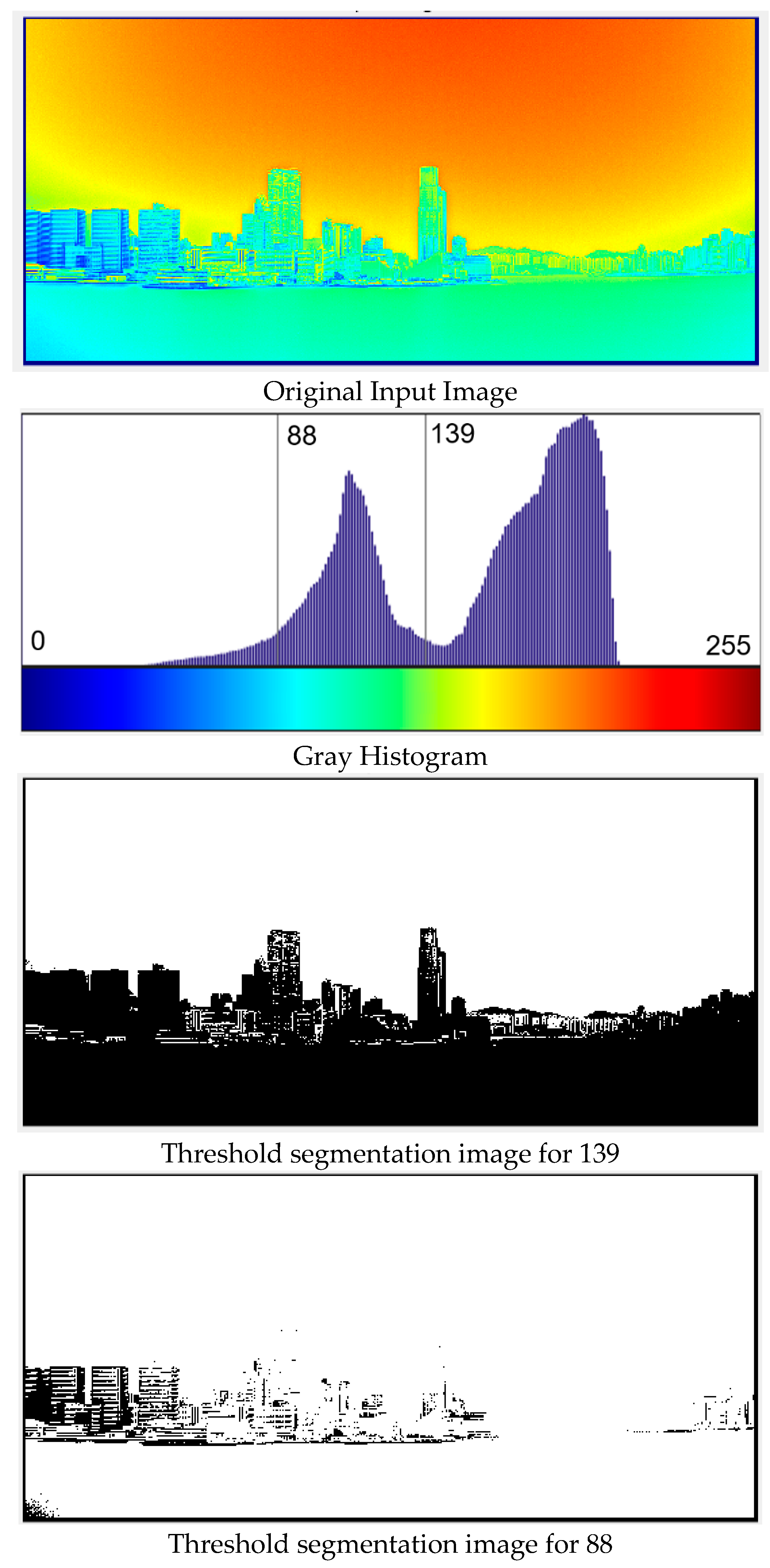
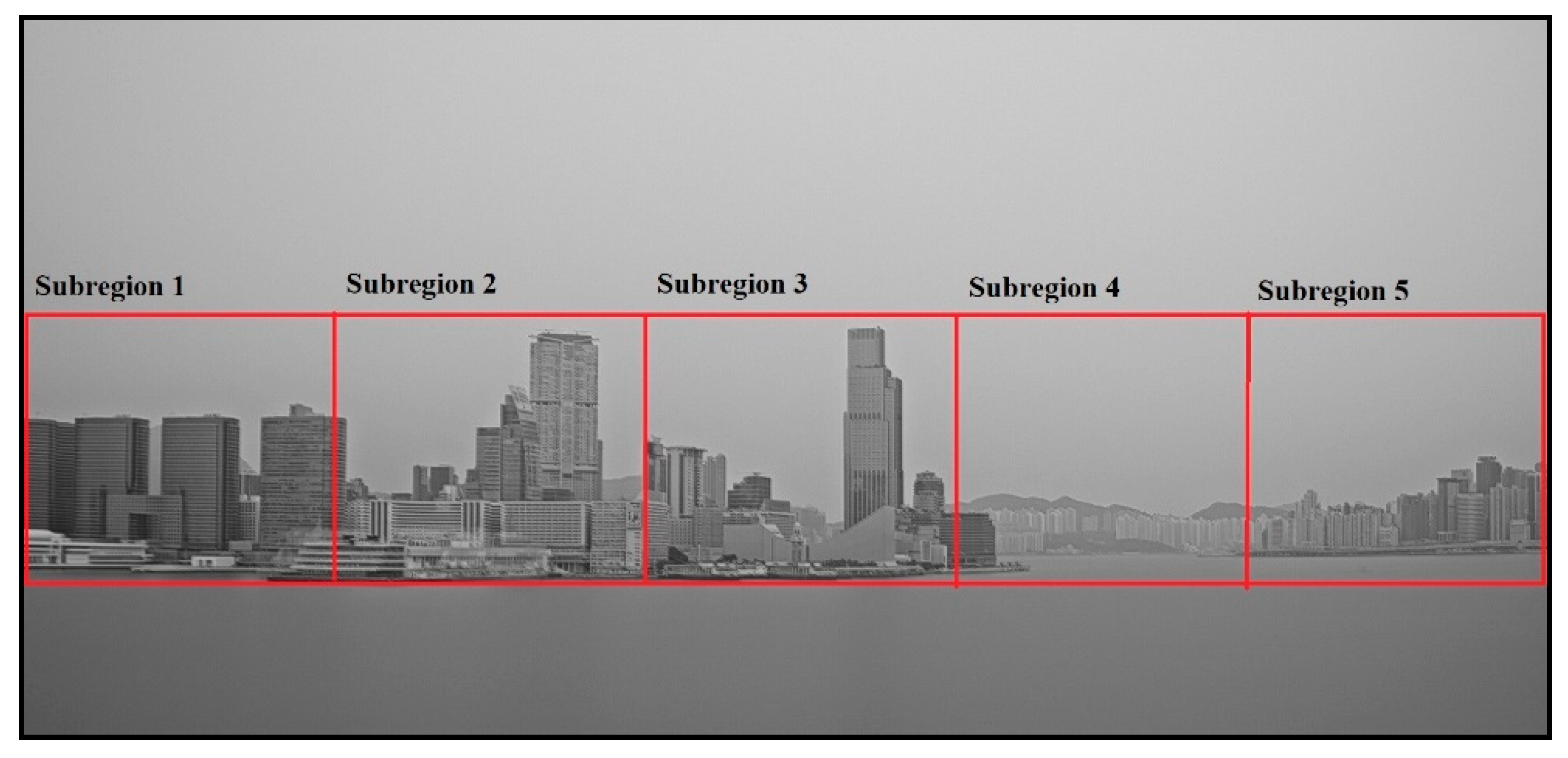
2.2.2. Subregion Segmentation

After obtaining the image with outlines of the buildings, it is necessary to segment the image into different detection subregions. Image segmentation is a popular method to divide an image into different feature regions for extracting the objects of interest [28,29]. Segmentation is a critical step connecting image processing and image analysis.

There were many threshold selection methods in the past research, among which the maximum between-class variance method was the most widely used [30]. However, this method has the limitation that the target object could not be segmented from the background when the method is applied to images with complex backgrounds. Hence, an adaptive threshold segmentation method had been proposed [31]. Instead of calculating global image thresholds, local thresholds were calculated based on the distribution of brightness in different regions of the image. For different regions of the image, it can calculate different thresholds adaptively [32]. Figure 7 showed the histogram of the gray-level averaged image. We used the gray-level distribution of the histogram to determine the threshold.

The adaptive threshold algorithm could be applied to image with uneven illumination. In order to compensate the differences in illumination, the brightness of each pixel needs to be normalized before determining whether the pixel was black or white. The gray-weighted average image derived in previous pre-processing steps was used as a reference. Adaptive threshold algorithm was used to determine the threshold value from which we could locate the area containing only fixed structure or buildings.

After applying the adaptive threshold algorithm, we have found two candidates for the threshold value (139 and 88 as shown in Figure 8). As the threshold value 88 can remove the background more effectively, segmentation threshold value of 88 is selected. According to the selected threshold value, the coordinates of the highest and lowest points of the effective area were located.

The image is then divided into segments with parallel lines as shown in Figure 9. We could find 5 effective subregions of similar size as shown in Figure 9 and image feature will then be extracted as described in the next session. In summary, the step-by-step procedures for the effective area extraction are described as follows.

• Apply gray-level averaging to all the images in the database to derive the comprehensive image.
• Gaussian blur algorithm was applied to the image to obtain the grayscale distribution of the image.
• Apply the adaptive threshold segmentation algorithm to find the threshold value.
• According to the threshold value found in step 3, the images in the database were then segmented into sub-region images with x-y coordinates.
• Effective subregions are then extracted from the results of step 4.

2.2.3. Subregion Feature Extraction and Visibility Evaluation

After obtaining the sub-regions, the features of the subregions are extracted to provide input variables for subsequent visibility estimation. The image of the sub-region contains lots of information and features, including features related to visibility estimation and other redundant information due to interference. If all the information of the sub-region image was directly mapped with the visibility value, the amount of data calculation for training was too large, and the redundant information may cause errors in the final results. Therefore, feature extraction was an indispensable and important step for the image of the subregions.

Feature extraction was one of the most important operations in image processing. It considered the image as a data set, and pixels’ features as elements. The process aims at finding the elements in the data set that could give the best representation of the data characteristics. According to different requirements of image classification and parameter evaluation, the method and dimension for feature extraction could be greatly different. In this paper, four common deep learning feature extraction methods based on the Keras-platform were used. These methods were (VGG)-16 network, (VGG)-19 network, DenseNet network and ResNet_50 network. The extracted features were used as the input variables for the visibility evaluation model, and the variables were used as input for the Support Vector Regression model, and then visibility evaluation was performed on the effective area.

2.2.4. Comprehensive Visibility Evaluation

The extracted sub-regions will be affected by various factors, such as image texture, structure and uneven light illumination. These factors will cause uncertainty or error in the final result. In order to obtain a more accurate final visibility estimation results, the weighted fusion method is applied to the visibility models of all the sub-regions [21]. Fusion method is summarized in Appendix B.

3. Experiment Results and Analysis

3.1. Experiment Platform

In order to evaluate the method proposed in this paper, we conduct experiments on the platform shown in

Table 2. The hardware and software parameters of the server.

Item	Configuration
Operating System	Linux
Memory Capacity	32GB memory
Central Processing Unit	2.6 GHz Intel CPU i7-8700
Graphics Processing Unit	NVIDIA GeForce GTX 1060 Ti
Software platform	Python 3.6
Deep Learning Library	Keras
Image database	Hong Kong Observatory (HKO)

. Here, the image resolution of Hong Kong Observatory (HKO) Image database is 1920 × 1080 pixels. The true value of visibility for each image to be trained comes from the visibility meter data provided by HKO. The dataset has a total number of 4841 selected images from database. We have selected 3630 images randomly as training set and the remaining 1211 images are selected as test set.

According to the needs of the experiment, each image could provide appropriate sub-regions through gray-scale average. The visibility distribution of the image database is shown in

Table 3. Visibilities distribution of the image database.

Image Database of Hong Kong Observatory	Visibility Range (km)
	0–10	11–20	21–30	31–40	40–50	Total
No. of training set sample images	432	1271	762	726	439	3630
No. of test set sample images	144	424	254	242	146	1210
Total	576	1695	1016	968	585	4841

.

3.2. Result and Analysis

In the experiment, the visibility of the test set images was evaluated according to the neural network-regression model. Through gray averaging and region segmentation, we had obtained the effective subregions. First, we performed the feature extraction on the extracted effective area, and then imported the extracted features into the support vector machine model for training. Finally, we obtained the predicted visibility value. Comparing the actual visibility value and the predicted visibility value in each effective subregion, we could get the visibility evaluation result of the effective subregions. By analyzing the error of each effective subregions, the fusion weight of each effective area can be obtained. The fusion weights were used for the fusion of the visibility evaluation model of all effective subregions. Finally, the comprehensive visibility of fusion could be obtained.

The organization of the sections for the results and analysis are summarized as follows. Among them, for different effective subregions, the results of model analysis of the visibility evaluation were shown in part (1). In order to verify the effectiveness of the method proposed in this paper more extensively, we have used different image features extracted from different networks, such as (VGG)-16 network, (VGG)-19 network, DenseNet network, ResNet-50 network. The extracted features were imported into support vector machines to train, and finally we got the visibility regression results. In part (2), we evaluated the performances of the four networks, (VGG)-16 network, (VGG)-19 network, DenseNet network and ResNet-50 network. The detailed experimental results were shown in part (2). In addition, in order to verify the performance of the method in different visibility ranges, we have evaluated the results for different visibility ranges in part (2). Finally, in order to compare the fusion methods, the experimental results under different fusion strategies were analyzed and discussed in part (3). In part (4), we compared the fusion effect of this paper with those in other papers.

(1)

Analysis of different effective areas

In order to assess the validity of the effective subregions, the visibility estimates and the subregion weights of each effective subregion were shown in

Table 4. The estimated results of different effective area.

No. of Effective Subregion	No.1	No.2	No.3	No.4	No.5
Estimated visibility	16.44	13.77	15.81	14.97	13.07
Fusion Weight	0.12	0.23	0.25	0.18	0.22

. The visibility of subregions with detailed objects, such as effective subregion No.3, No.4, and No.5 in Figure 10, was closer to the actual visibility. These subregions with rich details were weighted correspondingly higher than the blurred subregions. In order to assess the effect of the number of effective subregions on the estimation accuracy, the accuracies with different numbers of effective subregions were shown in

Table 5. Visibility accuracy of fusion of effective subregion.

	Fusion of Effective Subregion
No. of Effective subregion	No.1	No.1, No.3, No.5	No.1, No.2, No.3, No.4, No.5
Accuracy (%)	67.83	83.1	91.2

. The accuracy with the fusion of one effective subregion (No.1) and three effective subregions (No.1, No.2, and No.3) were much lower than that obtained by fusion of all five subregions (No.1–No.5). The main reason was that the larger the number of sub-regions, the higher the authenticity of the details in each effective sub-region, and the easier it was to be close to the true value. In addition, if the segmented single effective subregion was too large in scope, it had too many different levels of structure and details in that subregion, which would result in reduced sensitivity of the extracted features and thus reduced accuracy of the final detection. Likewise, if the extent of a single subregion was too small, the area containing too little hierarchical structure and detail would have limited validity and would not be as well differentiated in terms of visibility. All in all, according to the experimental results, it was more appropriate to divide the whole image into five subregions for experimental case in this paper.

(2)

Performance of different feature extraction networks

In order to verify the effectiveness of the proposed method in this paper, we have used different image features extraction networks, such as (VGG)-16 network, (VGG)-19 network, DenseNet network, and ResNet-50 network. The 512-dimensional feature vectors were extracted from the VGG-16 and VGG-19 networks. We extract the 1920-dimensional feature vectors from the DenseNet network. Feature vectors with 2048 entries were extracted from the ResNet_50 network as the coded features.

Table 6. Visibility accuracy of different networks.

Deep Learning Network	Visibility Range (km)
	0–10	11–20	21–30	31–40	41–50	Total
VGG-16 (%)	84.36	91.31	89.16	87.45	87.22	88.26
VGG-19 (%)	85.61	91.66	89.32	87.96	87.52	88.32
DenseNet (%)	89.41	93.22	92.31	88.51	88.10	90.52
ResNet_50 (%)	89.11	94.58	91.51	88.62	88.33	91.20

showed the visibility accuracy of these four networks in each visibility range. Although the overall accuracies of VGG-16 and VGG-19 network was 88%, the VGG-16 and VGG-19 networks gave lower accuracies in lower visibility range as compared with the DenseNet network and the ResNet-50 network.

As ResNet_50 and DenseNet networks were more sensitive to image attenuation and could provide valid image features at different visibility levels, it could increase the network’s extraction rate of valid features. These two networks would be more sensitive to provide valid features for visibility estimation regression. According to the experimental results, ResNet_50 network was recommended for image feature extraction, especially in the low visibility range. ResNet_50 network also had higher stability and robustness in other ranges.

(3)

Different fusion method

In order to assess the visibility estimation results for different fusion strategies, we have evaluated the following fusion strategies, namely the random fusion, the average fusion and the proposed weight fusion. In the random fusion method, any one effective subregion after image segmentation was selected randomly for the feature extraction and regression model analysis, and its visibility result was regarded as the final fusion result. In the average fusion method, the average value of all the estimates from different subregions was used as the final fusion result. In the weight fusion method, the fusion weight of each effective subregion was derived from the results of the error analysis. The accuracies of different fusion methods were shown in

Table 7. Visibility accuracy of different fusion strategies.

Fusion Method	Visibility Range (km)
	0–10	11–20	21–30	31–40	41–50	Total
Random fusion (%)	55.62	57.16	69.55	69.21	68.71	67.48
Average fusion (%)	78.39	80.95	88.79	87.46	86.58	84.53
Weight fusion (%)	86.12	93.61	92.25	92.21	91.60	90.32

.

According to the results of Table 7, random selection strategy give the poorest results. As the randomly selected method has not included sufficient feature values for visibility estimation. In random fusion method, only the features of the selected effective sub-region are used, which reduces the information for visibility evaluation, thereby affecting the final accuracy. Factors such as the uneven light illumination in the image may cause excessive errors in final estimated visibility value. Compared with the random fusion method, the average fusion method could give better performances in the range of 21–50 km as compared to the random fusion method. The performance of average fusion method in low visibility range (0–20 km) is still not satisfactory. On the other hand, the weight fusion method effectively fused the local estimates of the subregion images with the considerations of the fitted variances of the predicted distribution. Therefore, weight fusion can give better robustness and stability. In summary, weighted fusion method can give the best visibility estimation results for whole visibility range.

(4)

Comparison of different methods in other paper

As compared with the method in [25], the accuracy of visibility estimation in [25] was only about 80%. The effective subregions in [25] are selected based on pre-requisite landmark objects information and human judgement. The selection process is not from an objective approach of regression model analysis. Therefore, some important image information could be ignored after the subregion selection process. Furthermore, as only one single subregion is used for the visibility estimation by support vector machine (SVM), the accuracy is about 82% only. On the other hand, the accuracy of the proposed method in this paper can be about 90%. It shows that the effective subregions selection method proposed in this paper was more reasonable and the fusion method can give more accurate results.

As compared with the method in [21], the accuracy of visibility estimation in [21] can also reach 90%. However, the sub-regions are extracted based on equal division of image. Subregions’ selection by equal division of the whole image may have the following disadvantages. Useful image objects and the reductant image objects will be mixed and distribute among different subregions. As the proposed algorithm in [21] adjust the subregions image to the size of 224 × 3 × 224 after the division process, this will cause deformation of the subregion image and affect the estimation results. As the useful image information in the subregions is not extracted efficiently, this will increase the computation time.

The proposed method in this paper focus on more effective selection of subregions with useful static objects, it can reduce the area with reductant information in the subregions. The proposed method solves the problem of low data processing efficiency and low estimation accuracy, it can reduce the unnecessary computation load for the reductant image information in the image.

This proposed method can extract the effective subregions effectively and it can also provide reasonable accuracy for a wide estimation range with the uses of multiple SVR models and fusion method. The mapping surface between the visibility values and the feature vectors is complex and has high dimensions. By incorporating a number of piecewise SVR models, the multiple SVR models can approximate the highly dimension complex mapping surface of the visibility function.

4. Discussion and Summary

According to the results in Figure 10 and Section 3.2. It can be found that

• Each effective subregion R_i contains some static landmark objects at certain distances from observer location. Suppose R_i contains a nearest static object at distance x_i. If visibility is below x_i, all the objects in R_i cannot be observed and the whole region will be appeared as a uniform gray region as outline edges of the objects cannot be seen in this visibility range. Variations of image characteristics (e.g., gray level, and image sharpness of static objects) are observable for visibility range greater x_i and R_i can provide useful image feature information for visibility estimation in a visibility range above x_i.
• The weather images in this paper were collected in order of time sequence. Taking the hull as an example, the same hull will appear in different positions in the images. The entire image sequence records the moving trajectory of the hull from appearance to departure. Theoretically, a dynamic object must have a mean position from entering to departure. So long as the moving objects does not remain stationary at a certain position for a long time. These objects usually could be removed after the gray averaging process.
• The proposed method is even more effective for removing the natural moving objects in the nature such as moving clouds or sea waves. The area for the sky or the sea will become a uniform gray region after the gray averaging process. Therefore, after carrying out the proposed gray level averaging process, dynamic objects and natural moving objects could be removed in the image, leaving only the static objects in the image for subsequent region selection and feature extraction.
• In this case, if we perform the gray level averaging for the image dataset with visibilities higher than x_i. All static objects at distance less than x_i in R_i will be appeared as clear objects with sharp outline edges. Furthermore, dynamic objects (e.g., moving cloud and sea) will be filtered out if the total number of images is sufficiently large.
• In summary, performing gray level average on the entire image database could find static objects observable in different visibility ranges and locate the coordinates of the effective sub-regions. Combining with the threshold segmentation method, the gray level averaging can be used to detect observable static objects for different visibility ranges.
• The Feature Extraction and Regression model proposed in this paper is based on effective subregions selection, feature extraction by deep learning neural network, multiple support vector regression (SVR) models and weight fusion model for visibility estimation. Each support vector regression (SVR) model provide piecewise approximation for the overall complex mapping between visibility and image features.
• Different from other fusion methods as proposed in [21], the fusion in this paper aims to exclude invalid areas, reduce the amount of calculation and maintain the accuracy of visibility evaluation. Actually, the fusion approach in [21] does not exclude invalid regions, while the proposed method in this paper does not restrict the size and location of the subregions. It determines the segmentation of image according to the content of static objects in the whole image.
• In case the image contains no static objects in a particular visibility distance, visibility value at this range is estimated based on the interpolation (or fusion) of visibility values from other subregions.
• In summary, the proposed method can reduce the processing time of image features as only the selected regions are analyzed instead of the whole image. It can improve the estimation accuracy by using fusion for the estimates from different subregions. The proposed method shows good performance and results for the practical visibility data provided by HKO. Experimental results show that the accuracy of visibility estimation reaches more than 90%. This method did not need to define a large-scale visual annotation set, and had high robustness and effectiveness. This method also eliminates the interference of invalid regions and reductant features on the visibility estimation, and reduced the complexity and operations of the estimation process.

5. Conclusions

At present, deep neural networks have been widely used in the visibility estimation of weather images, but most methods do not focus on the features and content of the effective subregions. From the perspective of effective feature extraction, this paper looked for efficient selection of useful subregions and features extraction for the visibility estimation. This paper proposed a novel deep learning neural network method for the visibility estimation based on feature fusion method, which located the most effective image subregions by gray-level averaging. This proposed method used deep learning neural network to extract features and the established visibility models for each subregion by using Support Vector Machine (SVM). The visibilities of the sub-regions were fused together according to the results of the weight fusion analysis.

In the proposed method, all the images in the database were gray-weighted firstly to remove interference areas, in order to obtain the effective subregions. In this paper, five subregions were extracted for subsequent feature extraction. Four feature extraction networks (Densest, ResNet_50, Vgg16, and Vgg19) were used to extract features from the subregions. The features vectors obtained by the neural network were then imported into the proposed SVR regression models, in which the visibility functions with image features input are curve fitted by the SVR models. According to the results of the error analysis, the weight fusion was performed to derive the final visibility estimate.

This proposed method extracts valid and effective subregions to improve the training efficiency and estimation accuracy, it also solves the problem of long computation time due to the data processing of the whole image or equally divided subregions of the whole image. Since the effective subregions were derived by the gray average method during pre-processing, this process in performed only in the initialization stage. While the image processing is performed only for the selected effective subregions, image processing for the invalid and reductant area is avoid. Compared with other methods, this paper not only extracted the features of image efficiently, it shortened the data processing time for the whole process, and it improved the efficiency of model training, and avoided the interference of invalid features.

The major idea of the proposed subregions selection method is summarized as follows. As the distribution, number and location of static landmark objects in a digital image are depended on the actual physical environment, we cannot select the effective subregions arbitrarily. Suppose the image dataset are sorted in ascending order of visibility distances. We can identify the location of the nearest to farthest objects by performing the gray level average for the dataset from the smallest to the largest visibility distance. The major aim of the proposed selection method is to group a set of static landmark objects into a particular subregion so that the variation of its image characteristic is sensitive a particular visibility range. Hence, we can train a SVR model to curve fitted the visibility function with the input image features. By combining these SVR models by fusion method, we can estimate the final visibility by using the approximate multiple SVR model.

The proposed method gives good performances and accuracies in a range of 0–50 km which is suitable for practical applications. Experimental results show that the visibility estimation accuracy of the proposed method is more than 90%. It could be used to estimate the visibility value of the whole image, with high robustness and effectiveness. This method does not require to define a large-scale visual annotation set, and it also eliminates the processing of invalid and reductant information on the digital images as compared to other existing methods. For the fine-tuning of the neural network and extraction of effective subregions, it greatly reduces the model complexity and the computation time as compared to other methods.

Although our model could successfully evaluate the visibility of images accurately, it still had some limitations. In terms of calculation time, it was quite time-consuming to carry out the preprocessing and gray level averaging of the whole dataset to obtain the coordinates of the effective subregions. However, the preprocessing stage is only necessary during the initialization and pre-tuning stage. While the new images are taken by CCTV and added into dataset, the SVR models will be updated. In the case of increased application noise, this would affect the choice of the effective area. In addition, the fusion of the sub-region visibility assessment model proposed in this paper can reduce the effect of increased application noise to some extent.

Another limitation of the proposed method in this paper is that it is applicable to daytime images only. Further modifications of the algorithm are needed when it is applied to night-time images. These limitations will be further investigated in the future. In addition, in our future research, we will also focus on optimizing the selection of effective subregions. So as to minimize the number of subregions in a particular image dataset while the visibility estimation accuracy can be maintained at reasonable level.

References

1. Khademi, S.; Rasouli, S.; Hariri, E. Measurement of the atmospheric visibility distance by imaging a linear grating with sinusoidal amplitude and having variable spatial period through the atmosphere. J. Earth Space Phys. 2016, 42, 449–458. [Google Scholar]
2. Zhuang, Z.; Tai, H.; Jiang, L. Changing Baseline Lengths Method of Visibility Measurement and Evaluation. Acta Opt. Sin. 2016, 36, 0201001. [Google Scholar] [CrossRef]
3. Song, H.; Chen, Y.; Gao, Y. Visibility estimation on road based on lane detection and image inflection. J. Comput. Appl. 2012, 32, 3397–3403. [Google Scholar] [CrossRef]
4. Liu, N.; Ma, Y.; Wang, Y. Comparative Analysis of Atmospheric Visibility Data from the Middle Area of Liaoning Province Using Instrumental and Visual Observations. Res. Environ. Sci. 2012, 25, 1120–1125. [Google Scholar]
5. Minnis, P.; Doelling, D.R.; Nguyen, L.; Miller, W.F.; Chakrapani, V. Assessment of the Visible Channel Calibrations of the VIRS on TRMM and MODIS on Aqua and Terra. J. Atmos. Ocean. Technol. 2008, 25, 385–400. [Google Scholar] [CrossRef] [Green Version]
6. Chattopadhyay, P.; Ray, A.; Damarla, T. Simultaneous tracking and counting of targets in a sensor network. J. Acoust. Soc. Am. 2016, 139, 2108. [Google Scholar] [CrossRef]
7. Zhang, J.; Zhang, G.Y.; Sun, G.F.; Su, S.; Zhang, J.L. Calibration Method for Standard Scattering Plate Calibration System Used in Calibrating Visibility Meter. Acta Photonica Sin. 2017, 46, 312003. [Google Scholar] [CrossRef]
8. Huang, S.C.; Chen, B.H.; Wang, W.J. Visibility Restoration of Single Hazy Images Captured in Real-World Weather Conditions. IEEE Trans. Circuits Syst. Video Technol. 2014, 24, 1814–1824. [Google Scholar] [CrossRef]
9. Farhan, H.; Jechang, J. Visibility Enhancement of Scene Images Degraded by Foggy Weather Conditions with Deep Neural Networks. J. Sens. 2016, 2016, 3894832. [Google Scholar]
10. Ling, Z.; Fan, G.; Gong, J.; Guo, S. Learning deep transmission network for efficient image dehazing. Multimed. Tools Appl. 2019, 78, 213–236. [Google Scholar] [CrossRef]
11. Ju, M.; Gu, Z.; Zhang, D.; Qin, H. Visibility Restoration for Single Hazy Image Using Dual Prior Knowledge. Math. Probl. Eng. 2017, 2017, 8190182. [Google Scholar] [CrossRef] [Green Version]
12. Zhu, L.; Zhu, G.; Han, L.; Wang, N. The Application of Deep Learning in Airport Visibility Forecast. Atmos. Clim. Sci. 2017, 7, 314–322. [Google Scholar] [CrossRef] [Green Version]
13. Li, S.Y.; Fu, H.; Lo, W.L. Meteorological Visibility Evaluation on Webcam Weather Image Using Deep Learning Features. Int. J. Comput. Theory Eng. 2017, 9, 455–461. [Google Scholar] [CrossRef] [Green Version]
14. Chen, B.H.; Huang, S.C.; Li, C.Y.; Kuo, S.Y. Haze Removal Using Radial Basis Function Networks for Visibility Restoration Applications. IEEE Trans. Neural Netw. Learn. Syst. 2017, 29, 3828–3838. [Google Scholar] [PubMed]
15. Chaabani, H.; Werghi, N.; Kamoun, F.; Taha, B.; Outay, F. Estimating meteorological visibility range under foggy weather conditions: A deep learning approach. Procedia Comput. Sci. 2018, 141, 478–483. [Google Scholar] [CrossRef]
16. Palvanov, A.; Cho, Y.I. DHCNN for Visibility Estimation in Foggy Weather Conditions. In Proceedings of the 2018 Joint 10th International Conference on Soft Computing and Intelligent Systems (SCIS) and 19th International Symposium on Advanced Intelligent Systems (ISIS), Toyama, Japan, 5–8 December 2018. [Google Scholar]
17. You, Y.; Lu, C.; Wang, W.; Tang, C.K. Relative CNN-RNN: Learning Relative Atmospheric Visibility from Images. IEEE Trans. Image Process. 2018, 28, 45–55. [Google Scholar] [CrossRef]
18. Choi, Y.; Choe, H.G.; Choi, J.Y.; Kim, K.T.; Kim, J.B.; Kim, N.I. Automatic Sea Fog Detection and Estimation of Visibility Distance on CCTV. J. Coast. Res. 2018, 85, 881–885. [Google Scholar] [CrossRef]
19. Ren, W.; Pan, J.; Zhang, H.; Cao, X.; Yang, M.H. Single Image Dehazing via Multi-scale Convolutional Neural Networks with Holistic Edges. Int. J. Comput. Vis. 2019, 128, 240–259. [Google Scholar] [CrossRef]
20. Lu, Z.; Lu, B.; Zhang, H.; Fu, Y.; Qiu, Y.; Zhan, T. A method of visibility forecast based on hierarchical sparse representation. J. Vis. Commun. Image Represent. 2019, 58, 160–165. [Google Scholar] [CrossRef]
21. Li, Q.; Tang, S.; Peng, X.; Ma, Q. A Method of Visibility Detection Based on the Transfer Learning. J. Atmos. Ocean. Technol. 2019, 36, 1945–1956. [Google Scholar] [CrossRef]
22. Outay, F.; Taha, B.; Chaabani, H.; Kamoun, F.; Werghi, N. Estimating ambient visibility in the presence of fog: A deep convolutional neural network approach. Pers. Ubiquitous Comput. 2019. [Google Scholar] [CrossRef]
23. Zhang, C.; Wu, M.; Chen, J.; Chen, K.; Zhang, C.; Xie, C.; Huang, B.; He, Z. Weather Visibility Prediction Based on Multimodal Fusion. IEEE Access 2019, 7, 74776–74786. [Google Scholar] [CrossRef]
24. Palvanov, A.; Cho, Y. VisNet: Deep Convolutional Neural Networks for Forecasting Atmospheric Visibility. Sensors 2019, 19, 1343. [Google Scholar] [CrossRef] [PubMed] [Green Version]
25. Lo, W.L.; Zhu, M.; Fu, H. Meteorology Visibility Estimation by Using Multi-Support Vector Regression Method. J. Adv. Inf. Technol. 2020, 11, 40–47. [Google Scholar]
26. Malm, W.; Cismoski, S.; Prenni, A.; Peters, M. Use of cameras for monitoring visibility impairment. Atmos. Environ. 2018, 175, 167–183. [Google Scholar] [CrossRef]
27. De Bruine, M.; Krol, M.C.; van Noije, T.P.C.; Le Sager, P.; Röckmann, T. The impact of precipitation evaporation on the atmospheric aerosol distribution in EC-Earth v3.2.0. Geosci. Model Dev. Discuss. 2017, 11, 1443–1465. [Google Scholar] [CrossRef] [Green Version]
28. Hautiére, N.; Tarel, J.P.; Lavenant, J.; Aubert, D. Automatic fog detection and estimation of visibility distance through use of an onboard camera. Mach. Vis. Appl. 2006, 17, 8–20. [Google Scholar] [CrossRef]
29. Yang, W.; Liu, J.; Yang, S.; Guo, Z. Scale-Free Single Image Deraining Via Visibility-Enhanced Recurrent Wavelet Learning. IEEE Trans. Image Process. 2019, 28, 2948–2961. [Google Scholar] [CrossRef]
30. Cheng, X.; Yang, B.; Liu, G.; Olofsson, T.; Li, H. A variational approach to atmospheric visibility estimation in the weather of fog and haze. Sustain. Cities Soc. 2018, 39, 215–224. [Google Scholar] [CrossRef]
31. Zhang, H.; Zhang, T.; Pedrycz, W.; Zhao, C.; Miao, D. Improved Adaptive Image Retrieval with the Use of Shadowed Sets. Pattern Recognit. 2019, 90, 390–403. [Google Scholar] [CrossRef]
32. Chaabani, H.; Kamoun, F.; Bargaoui, H.; Outay, F. A Neural network approach to visibility range estimation under foggy weather conditions. Procedia Comput. Sci. 2017, 113, 466–471. [Google Scholar] [CrossRef]
Figure 1. Flow Chart of Comprehensive Visibility Evaluation.
Applsci 11 00997 g001
Figure 2. Steps of Image Preprocessing.
Applsci 11 00997 g002
Figure 3. Some image samples in the database.
Applsci 11 00997 g003
Figure 4. Comprehensive image after gray weighted average.
Applsci 11 00997 g004
Figure 5. Image with grayscale 50–100.
Applsci 11 00997 g005
Figure 6. Comprehensive image of gray mean square error.
Applsci 11 00997 g006
Figure 7. Gray histogram of Comprehensive image after gray weighted average.
Applsci 11 00997 g007
Figure 8. Threshold segmentation image after gray weighted average.
Applsci 11 00997 g008
Figure 9. Subregion segmentation image.
Applsci 11 00997 g009
Figure 10. Example images of five subregions at different visibility range.
Applsci 11 00997 g010