1. Introduction
Maintenance activities in industrial systems are important in order to reduce product or system life-cycle costs. Corrective maintenance is an important type of maintenance activity that involves troubleshooting observed failures. Troubleshooting a failure involves identifying its root cause and performing repair actions in order to return the system to a healthy state.
In this work, we propose a novel troubleshooting algorithm that reduces troubleshooting costs by using an integration of diagnosis and prognosis techniques. Diagnosis deals with understanding what has happened in the past that has caused an observed failure. Prognosis deals with predicting what will happen in the future, and in our context, when future failures are expected to occur. In particular, we consider prognosis techniques that generate survival curves of components. These are curves that plot the likelihood of a component to survive (i.e., not fail) as a function of the components usage or age [
1]. There are analytical methods for creating survival curves and sophisticated machine learning techniques that can learn survival curves from data [
2].
Our first main contribution is to present a diagnosis algorithm that integrates prognostic information, given in the form of survival curves, with diagnostic information about the relations between sensor data and faults. To motivate this integration, consider the following illustrative example. A car does not start and the mechanic inspecting the car observes that the water level in the radiator is low. The mechanic at this stage has three possible explanations (diagnoses) for why the car does not start: either the radiator is not functioning well, the ignition system is faulty, or the battery is empty. Let , , and refer to these diagnoses, respectively. Assume that when the car does not start and the water level is low, the most likely diagnosis is, in general, . However, if the battery is old then becomes the most likely diagnosis. Thus, considering the age of the battery and the survival curve of batteries of the same type can provide valuable input for the mechanic in deciding the most likely diagnosis and the consequent troubleshooting action. We present a method for considering such prognostic information to improve diagnostic accuracy.
Most prior work on automated troubleshooting aimed to reduce the costs incurred during the current troubleshooting process [
3], while ignoring future maintenance costs. Future maintenance costs include costs due to future failures, which would require additional troubleshooting actions and perhaps system downtime. Our second main contribution is introducing a novel type of troubleshooting problem in which the aim is to minimize current and future troubleshooting costs. We refer this type of troubleshooting as anticipatory troubleshooting. We propose several anticipatory troubleshooting algorithms that explicitly consider future costs by considering survival curves.
Considering future costs in a troubleshooting process raises two main dilemmas. The first dilemma is the fix–replace dilemma: whether to fix a broken component or replace it with a new one. Fixing a faulty component is usually cheaper than replacing it with a new one, but a new component is less likely to fail in the near future. The second dilemma is the replace-healthy dilemma: whether to replace an old but healthy component now in order to save the overhead costs of replacing it later, when it becomes faulty.
To motivate those dilemmas, consider again a scenario in which a car does not start. The mechanic finds out that the gear box is broken and must be repaired. The first dilemma deals with the decision of whether to fix the current, faulty gear box or replace it with a new one. Fixing the current gear box is often cheaper than replacing it with a new one, but a new gear box is expected to stay healthy longer. This is the fix–replace dilemma.
As a motivating example for the second dilemma, consider the case that while the mechanic inspects the broken gear box, he also observes that the car’s clutch is worn out. While it is not broken now, it looks like it might break in the near future. At this stage we are faced with the replace-healthy dilemma: should we replace the clutch now or not? Choosing not to replace the clutch now obviously reduces the cost of the current garage visit, but one may end up incurring a significantly higher cost in the future if not, as it would require towing the car again to the garage and moving the gear box again in order to reach the clutch.
We provide a principled and unified manner to address both dilemmas, by modeling them as a single Markov decision process (MDP). The MDP is a well-known model for decision making that is especially suitable for domains with uncertainty in which reasoning about future events is necessary. By modeling our dilemmas as an MDP, we allow solving them with an MDP solver and determine whether to fix or replace and whether to replace healthy components.
The MDP that accurately describes our dilemmas is very large, and therefore hard to solve. Therefore, we propose an efficient heuristic algorithm that under some assumptions can still minimize the expected troubleshooting costs over time. We evaluated our MDP-based algorithm and our heuristic algorithm experimentally on benchmark systems modeled by Bayesian networks [
4]. Results show that the heuristic algorithm demonstrates significant gains compare to baseline policies, and that the MDP approach significantly reduces the long-term maintenance cost. Additionally, we show that considering the replace-healthy dilemma enables one to further reduce the long-term troubleshooting cost by up to 15 percent.
This work is an extension of our previous work, published in IJCAI-16 [
5]. In that version we presented only a heuristic algorithm. Beyond providing more detailed explanations of the fix–replace dilemma, we present here three significant contributions: (1) we present the replace-healthy dilemma, (2) we present an MDP solution for both dilemmas, and (3) we evaluate the MDP approach by comparing it to the simple heuristic we presented in the previous version of this paper [
5]. We show that the MDP approach significantly reduces troubleshooting costs.
2. Traditional Troubleshooting
In this section, we formalize the troubleshooting problem. A system is composed of a set of components, denoted COMPS. At any given point in time, a component can be either healthy or faulty, denoted by and , respectively. The state of the system, denoted , is a conjunction of these health predicates, defining for every component whether it is healthy or not. A system is in a healthy state if all its components are healthy, and in a faulty state if at least one component is faulty. A troubleshooting agent is an agent tasked to return the system to a healthy state. The agent’s belief about the state of the system , denoted , is also a conjunction of health literals. We assume that the agent’s knowledge is correct but possibly incomplete. That is, if or then or , respectively. However, there may exist a component such that neither nor is in . That is, it always holds that .
Following Heckerman et al. [
3] we assume the troubleshooting agent has two types of actions: sense and repair. Each action is parametrized by a single component
C. A sense action, denoted
Sense, checks whether
C is healthy or not. A repair action, denoted
Repair, results in
C being healthy. (See Stern et al. [
6] for a discussion on actions that apply to a batch of components). That is, applying
Sense adds
to
if
, and adds
to
otherwise. Similarly, applying
Repair adds
to both
and
, and removes
from
and
if it is there.
A troubleshooting problem arises if the system is identified as faulty. A solution to a troubleshooting problem is a sequence of actions performed by the troubleshooting agent, after which the system is returned to a healthy state.
Definition 1 (Troubleshooting Problem (TP)). A TP is defined by the tuple P = where (1) COMPS is the set of components in the system, (2) ξ is the state of the system, (3) B is the agent’s belief about the system state, and (4) is the set of actions the troubleshooting agent is able to perform. A TP arises if . A solution to a TP is a sequence of actions that results in a system state in which all components are healthy.
A troubleshooting algorithm (TA) is an algorithm for generating a sequence of actions that is a solution to a given TP. TAs are iterative: in every iteration the TA accepts the agent’s current belief B as input and outputs a sense or repair action for the troubleshooting agent to perform. A TA halts when the sequence of actions it has outputted forms a solution to the TP. That is, if an agent performs these actions, then the system will be fixed. Both sense and repair actions incur costs. The cost of an action a is denoted by . The cost of solving a TP using a solution , denoted by , is the sum of the costs of all actions in : . TAs aim to minimize this cost.
Consider the troubleshooting process example mentioned in
Table 1, in which a car does not start: The car is composed of three relevant components that may be faulty: the radiator (
), the ignition system (
), and the battery (
). Assume that the radiator is the correct diagnosis, meaning the radiator is really faulty, and the agent knows that the battery is not faulty. The corresponding system state
and agent’s belief
B are:
and
.
Table 1 lists a solution to this TP, in which the agent first senses the ignition system, then the radiator, and finally repairs the radiator.
Consider the case where the cost of sense actions is much smaller than the cost of repair actions. This simplifies the troubleshooting process: perform sense actions on components until a faulty component is found, and then repair it. The challenge in this case is which component to sense first.
To address this challenge, efficient troubleshooting algorithms use a diagnosis algorithm (DA). A DA outputs one or more diagnoses, where a diagnosis is a hypothesis about which components are faulty. These components will be sensed first.
Model-based diagnosis (MBD) is a classical approach to diagnosis in which a model of the system together with observations of the system’s behavior are used to infer diagnoses. Some MBD algorithms assume a system model that represents the system’s behavior using propositional logic. They use logical reasoning to infer diagnoses that are consistent with the system model and observations [
7,
8,
9,
10,
11,
12,
13].
In this work, we assume the available model of the system is a Bayesian network (BN) that represents the probabilistic dependency between observations and the system’s health state [
14]. Briefly, such a BN consists pf three disjoint sets of nodes: (1) control nodes, whose values depend only on the user’s actions; (2) sensor nodes, whose values represent data that can be observed from the system sensors; and (3) health nodes, whose values represent the state—healthy or some faulty state—of the system’s components. The observations of the system’s behavior are assignments of values to the control and at least some of the sensor nodes. A diagnosis is an assignment of values to the health nodes. The likelihood of a diagnosis
can be computed by running a BN inference algorithm such as variable elimination to compute the marginal probabilities of the health node assignments represented by
. The probability of each component
to be faulty, denoted by
, also can be derived [
15].
3. Troubleshooting with Survival Analysis
Beyond the literature on automated diagnosis, there is much work on developing prognosis techniques for estimating the remaining useful life of components in a system. Obviously, considering more information, such as the remaining useful lives of components, can provide valuable input to the troubleshooter towards figuring out the most likely diagnosis, and consequently the next troubleshooting action. In
Section 3.1, we introduce survival functions and in
Section 3.2 we explain how to integrate survival functions in the diagnosis process.
3.1. Survival Functions
Survival functions give the probability that a device, a system component, or other object of interest will survive beyond a specified time. Survival functions can be obtained by analysis of the physics of the corresponding system [
1] or learned from past data [
2].
Definition 2 (Survival Function). Let be a random variable representing the age at which C will fail. A survival function for C, denoted , is the cumulative distribution function of , that is: .
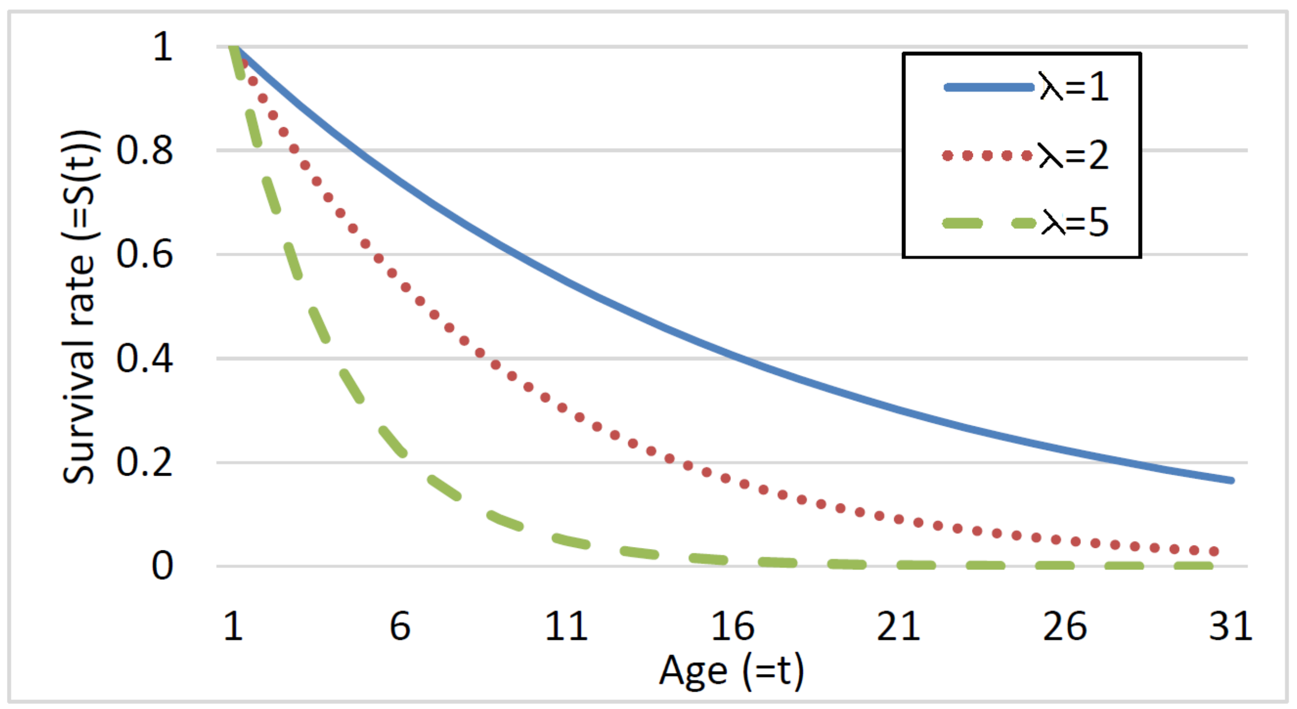
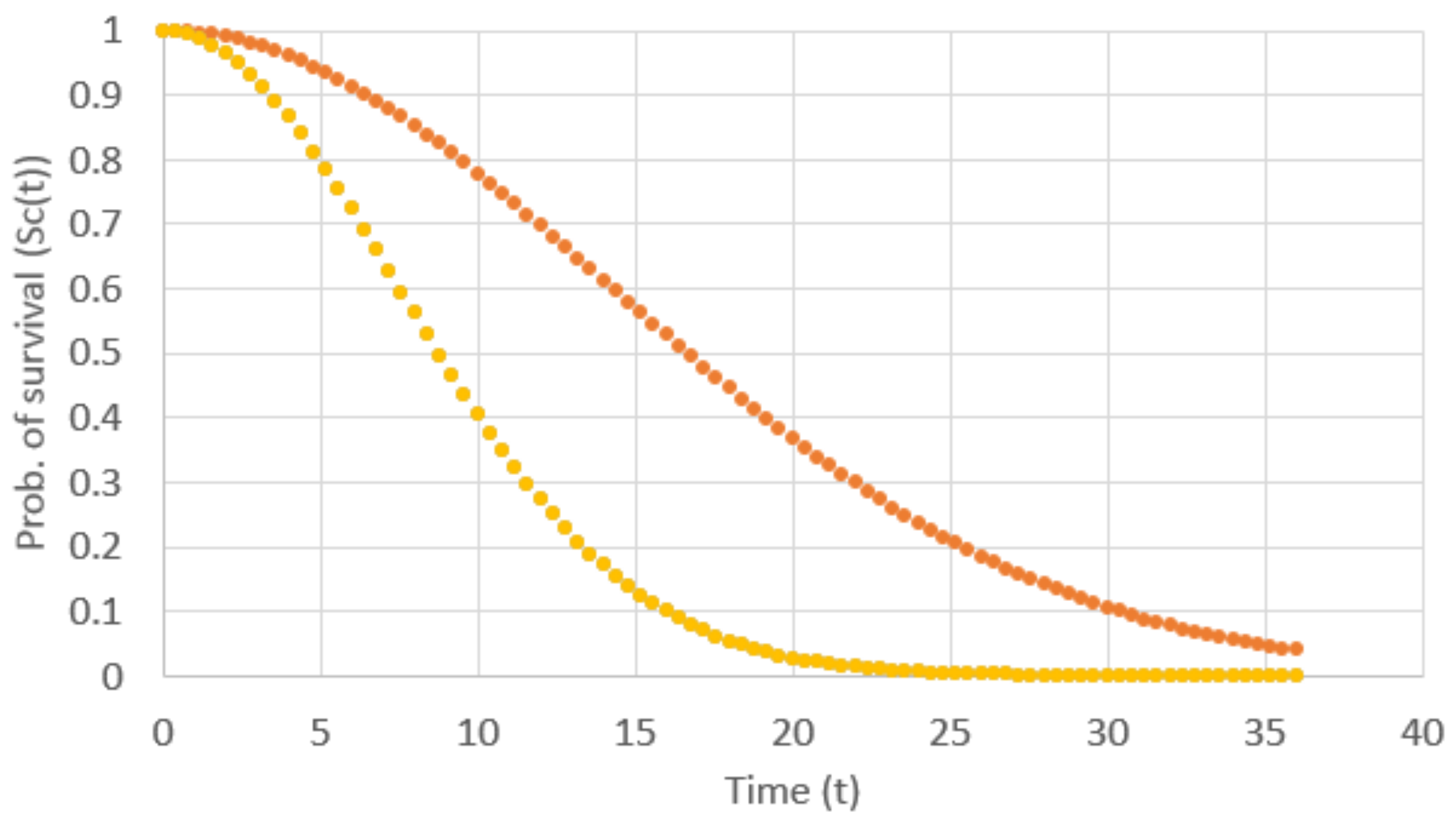
Figure 1 illustrates three possible survival curves generated by a Weibull decay function
where
t is the age (the
x-axis). The
y-axis represents the probability that a component will survive (i.e., not fail)
t time units (e.g., months).
and
b are parameters.
is known as the rate parameter in a Poisson process, and is related to the expected number of events occurring in a bounded region of time. In our case it represents the failure rate. The
b parameter is known as the hazard rate. This parameter depicts the instantaneous rate in which events occur. The three curves plotted in
Figure 1 correspond to the case that
and three values of the
parameter. Note that small
is associated with a higher probability to survive longer, whereas large
results in a lower probability to survive for a long time. An increasing hazard rate is appropriate since we expect younger components to be more likely to survive, i.e., to have the derivative of the survival function decrease as the component’s age increases.
The challenge is how to compute the probability that a component C caused a system failure given its age and survival function. In most systems, faulty components fail intermittently; i.e., a component may be faulty but acts normally. Thus, the faulty component that caused the system to fail may have been faulty even before time t. Therefore, we estimate the probability of a component C of age to have caused the system failure by the probability that it has failed any time before the current time. This probability is directly given by .
3.2. Integrating Survival Functions to Improve Diagnosis
For a given component C we have two estimates for the likelihood that it is correct: one from the MBD algorithm () and one from its survival curve (). The MBD algorithm’s estimate is derived from the currently observed system behavior and knowledge about the system’s structure. The survival curve estimate is derived from knowledge about how such components tend to fail over time. We propose to combine these estimates to provide a more accurate and more informed diagnostic report.
A simplistic approach to combine these fault likelihood estimates is by using some weighted linear combination, such that the weights are positive and sum up to one. However, we argue that these estimates are fundamentally different:
is an estimate given a priori to the actual fault, while
is computed by the MBD algorithm for the specific fault at hand, taking into consideration the currently observed system behavior. Indeed, MBD algorithms often require information about the prior probability of each component to be faulty when computing their likelihood estimates [
9,
16,
17,
18,
19,
20]. These priors are often set to be uniform, although it has been shown that setting such priors more intelligently can significantly improve diagnostic accuracy [
21,
22]. Therefore, we propose to integrate the fault likelihood estimation given by the survival curves as part of the priors within the likelihood estimation computation done by the MBD algorithm. We explain how this is done next.
Recall that every component
C is associated with a node
in the BN, such that the value of this node represents the health state of
C. Let
be the value of
representing that
C is healthy, and let
represent the other, non-healthy possible states of
C. Let
be the prior probability that
C is in state
. The sum of these priors, i.e.,
, expresses the a priori belief that the component is faulty, i.e., the belief before any evidence is taken into account. We propose to integrate the information into the survival curves with the health nodes’ priors, by introducing a revised prior for state
, denoted by
, which is defined as follows:
The intuition behind the formula is that the prior probability for being in a healthy state () can be computed by the survival function given the age of the component. The priors of the other faulty states are normalized by so that they sum up to one, but still preserve their relative prior probabilities from the BN.
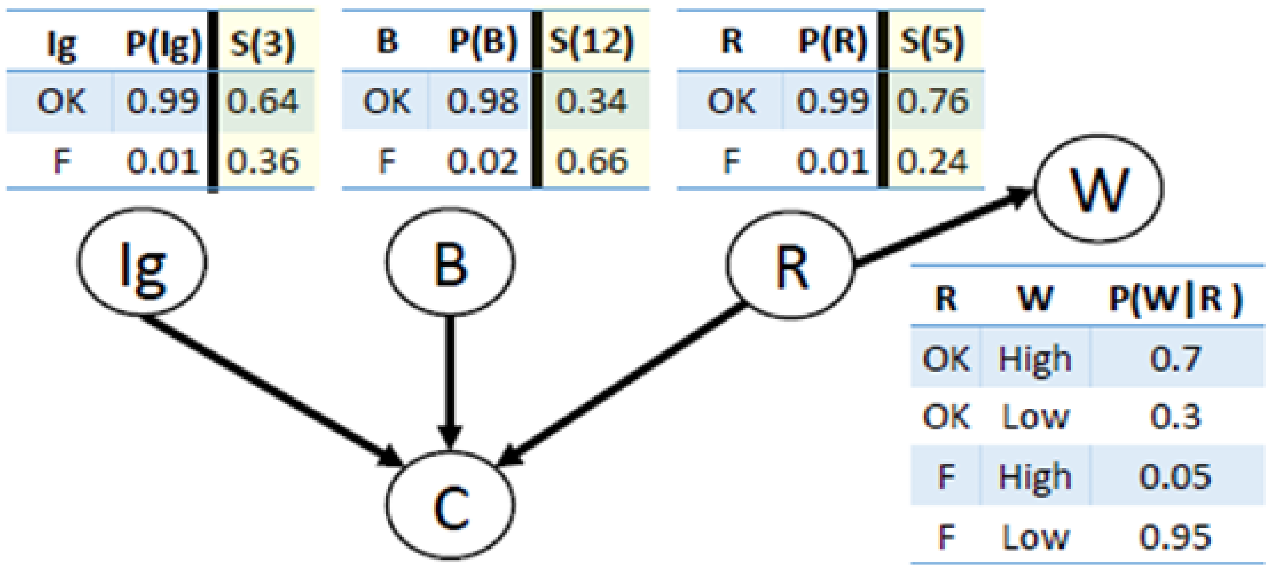
As an example of this integration of survival curves and diagnostic model, consider an MBD problem for a car.
Figure 2 depicts the BN we use as a system model for this car. Nodes
,
B, and
R correspond to the health variables for the ignition, battery, and radiator, respectively.
W corresponds to the water level variable, and
C corresponds to the observable variable that is true if the car starts properly and false otherwise. The conditional probability tables (CPTs) for all nodes except
C are displayed in
Figure 2. For example, the a priori probability that the ignition (
) is faulty is 0.01. The value of
C deterministically depends on
,
B, and
R: the car can start; i.e.,
C is true, if and only if all the components
,
B, and
R, are healthy. Modeling such dependency (a logical OR) in a BN is trivial. For simplicity, assume that at most one component—
,
B, or
R, can be faulty at a time. This is called the single-fault assumption. In general, we limit our discussion in this paper to the single-fault case. In
Section 8 we discuss how to extend our approach to multiple-fault scenarios.
Now, consider the case where the car does not start () and the water level is low (). Given this evidence, we apply Bayesian reasoning to get the likelihood of each component to be faulty. The likelihoods obtained for , B, and R to be faulty are 0.16, 0.33, and 0.52, respectively. Thus, an intelligent troubleshooter would sense R first.
Now, assume that the ages of the ignition (
), battery (
B), and radiator (
R) are 3, 12, and 5 months, respectively, and that they all follow an exponential survival curve
. Thus, based on the components’ ages and the survival curves the probabilities of
,
B, and
R being faulty are 0.24, 0.66, and 0.36, respectively. By adjusting the priors for
,
B, and
R using Equation (
1) and the given survival curves, we get the priors shown in
Figure 2. Setting these priors dramatically affects the result of the Bayesian inference, where now the probabilities of
,
B, and
R to be faulty are 0.16, 0.56, and 0.28, respectively. As a result, a troubleshooter that is aware of both BN and survival curves would choose to sense the battery (
B) rather than the radiator (
R).
In
Section 6, we demonstrate experimentally the benefit of integrating the survival functions in the BN inference process, showing significant gain.
4. Anticipatory Troubleshooting
As mentioned in the introduction, given a failure in a system, a traditional troubleshooting process aims to repair the failure while minimizing troubleshooting costs. The target of anticipatory troubleshooting is the same but also considers future troubleshooting costs.
Formally, let be the time interval in which we aim to minimize troubleshooting costs. During this time interval, several components may fail at different points in time, resulting in several TPs that must be solved. The target function we wish to minimize is the sum of costs incurred by the troubleshooting agent when solving all the TPs that occur throughout the designated time interval. We refer to this sum of troubleshooting costs as the long-term troubleshooting cost. An anticipatory troubleshooting algorithm is an algorithm that aims to minimize these costs.
Next, we discuss and study the following two dilemmas that arise during troubleshooting and for which using an anticipatory troubleshooting algorithm can be useful.
We describe these dilemmas in more detail below.
4.1. The Fix or Replace Dilemma
The first dilemma arises when there is more than one way to repair a faulty component. In particular, consider having two possible repair actions:
, which means the troubleshooting agent replaces C with a new one.
, which means the troubleshooting agent fixes C without replacing it.
Both fix and replace are repair actions, in the sense that after performing them the component is healthy and the agent knows about it, i.e., replacing with in both the system state and the agent’s belief. We expect fix and replace to differ in two important aspects.
First, the cost of replacing a component
C is likely to be different than the the cost of fixing an existing component—i.e.,
. Second, we expect the probability that a component
C will fail in the future changes after it is fixed. Formally, we define the
AfterFix curve of a component
C for time
, denoting
as
and expect that
A common setting is that (1) getting a new component is more costly than fixing it, and (2) a new component is less likely to fail compared to a fixed component. This setting is captured by the following inequalities:
This setting embodies the fix–replace dilemma in anticipatory troubleshooting: weighing current troubleshooting costs (according to which a fix is preferable) against potential future troubleshooting costs (according to which a replacement is preferable). All the algorithms proposed in this work are applicable beyond this setting, e.g., for cases where replacing a component is cheaper than fixing it.
4.2. The Replace Healthy Dilemma
System failures usually incur overhead costs, in addition to the cost of the repair actions, such as transportation costs (bringing the car to the garage) and system decomposition costs (disassembling the wheels and brakes). We denote by the overhead costs incurred by a single system failure.
When this overhead cost is non-negligible, it is worthwhile to consider replacing healthy components during a troubleshooting process in order to prevent them from failing in the future. For instance, if the car is anyway in the garage and treated by a mechanic, replacing the break pads now instead of in approximately three months saves the overhead costs of bringing the car to the garage again and disassembling the wheels and brakes. More generally, during a troubleshooting process, the troubleshooting agent has two possible actions for every healthy component C:
Naturally, does not incur any cost, but incurs . However, replacing a component might save future system failures, since the probability of having another failure in the same component after replacing it is lower than this probability when ignoring it. Thus, performing may end up saving future overhead costs. We call this dilemma of whether to repair a healthy component or not the replace-healthy dilemma.
5. Solving the Dilemmas
In this section, we propose two approaches for solving the fix–replace and replace-healthy dilemmas. The first approach is based on a simple heuristic decision rule (
Section 5.1) designed for the fix–replace dilemma. The second approach models each dilemma as a Markov decision process (MDP) problem and solves it with an MDP solver (
Section 5.2).
5.1. Solving the Dilemmas with Heuristic Rules
The heuristic decision rule described next, which we refer to as DR1, is a solution to the fix–replace dilemma. The input to DR1 is a tuple where: (1) C is a faulty component, (2) t is the current time, (3) is the age of C, (4) is the survival curve of C, and (5) is the survival curve of C if it is fixed at time t. DR1 outputs a repair action—either Fix(C) or Replace(C).
Definition 3 (
DR1)
. DR1 returns Replace(C) if the following inequality holds, and Fix(C) otherwise. DR1 is optimal if the following assumptions hold:
A component will not fail more than twice in the time interval .
A component can be fixed at most once.
A replaced component will not be fixed in the future.
Components fail independently.
We can not replace healthy components.
Explanation: If components fail independently (Assumption 4), it is sufficient to compare the long-term troubleshooting costs resulting from current and future failures of C, as C neither affects nor is affected by any other component. The long-term troubleshooting costs consist of the current cost of repairing C plus the costs of repairing C should it fail before . The current cost is or if C is fixed or replaced, respectively. Since we assume that a component will not fail more than twice (Assumption 1), computing the expected future troubleshooting costs is reduced to the probability that C will fail again before times the cost of replacing C if it fails (Assumption 2 and 3). The probability that C will fail before is if we fix C now, and if we replace it.
DR1 can be also applied when the assumptions do not hold, but then
DR1 may be non-optimal. Still, as we show experimentally in
Section 6, using
DR1 can be very beneficial.
5.2. Anticipatory Troubleshooting Dilemmas as a Markov Decision Process
Next, we propose a different approach to solve the fix–replace dilemma, and then show how it can also be adapted to solve the replace-healthy dilemma. This approach is based on modeling both dilemmas as Markov decision process (MDP) problems. In general, an MDP is defined by:
A set of states .
An initial state I.
A set of actions that are available from state s, for each state .
A transition function r. This is the probability that performing action a in state s will lead to state .
A reward function . This is the immediate reward received after performing action a in state s.
Next, we show how each dilemma can be modeled as an MDP.
5.2.1. Fix–Replace Dilemma as an MDP
To model the fix–replace dilemma as an MDP, we first discretize the time limit by partitioning it to n non-overlapping time intervals of size . Let be the time steps such that , and for all , is the time step that is the upper limit of time interval. Thus, . The number of time intervals (n) is referred to as the granularity level. The granularity level should be set according to the domain such that it provides a sufficient approximation of real failure times.
Finally, we can present our modeling of the fix–replace dilemma for component C.
States. A state in our MDP is a tuple , where:
is a time step.
IsFaulty is true iff C is faulty in the time interval .
is the survival curve of C at time .
is the age of C at time .
States for time represent the first time step. States for time are terminal states. Recall that we only consider single fault scenarios—i.e, at most one component fails.
Actions. The set of actions in our MDP consists of two actions:
Replace(C) and
Fix(C). The outcome of applying an action in a state
results in one of the two following states:
and
.
represents the state where component
C fails in the next time interval, and
represents the state where component
C does not fail in the next time interval. The values of
and
depend on the performed action. Applying
Replace(C) in state
s does not change the survival curve of
C, and sets the age of
C to zero at time
. Applying
Fix(C) in state
s does not change the age of
C but sets
to be the
AfterFix curve of
C. The columns
Fix(C) and
Replace(C) in
Table 2 provide a summary of how
and
are set after performing a repair action in a state
s.
Transition function. The transition function
for our MDP returns zero for any state
. The probability of reaching
, i.e., the probability that
C will fail in the time interval
, is computed based on
and
as follows.
which is a standard computation in survival analysis: the probability of surviving until
(when the age of
C is
) minus the probability of surviving until
(when the age of
C is
). As noted above, the outcome of applying any action
a to any non-terminal state
s is either
or
; we have that
.
Reward function. The reward function of our MDP is the negation of the cost of the executed action and the overhead cost, i.e., . We denote by the MDP defined above.
5.2.2. Replace-Healthy Dilemma as an MDP
Next, we describe our approach to model the replace-healthy dilemma as a set of MDPs. For every healthy component C, we define the following MDP designed to decide whether it is worthwhile to replace C or not at this stage.
States and actions. A state in this MDP is defined exactly a state in . The set of actions in this MDP is also the same as in , except for the actions in the initial state. In this state, we allow one of the following two actions: Replace(C) and Ignore(C). Ignore(C) means we decide not to replace C at the current time step. Note that there is no Fix(C) option here since C is currently healthy.
Transition function. As in
, applying an action has two possible outcomes: either
C is faulty in the next time interval or not, denoted
and
, respectively. The values of
and
after
Replace(C) or
Fix(C) are exactly the same as in
. After performing
Ignore(C), the corresponding survival curve does not change and the age increases with time. The row for
Ignore(C) in
Table 2 describes these changes in
and
in a formal way. The transition function
is exactly the same as in
:
Reward function. The reward function of this MDP is the negation of the cost of the executed action. For Replace(C), this cost is . Note that we do not add here the overhead cost, since the replace-healthy dilemma arises when already in a troubleshooting process. Obviously, the cost of Ignore(C) is zero.
5.2.3. Solving the MDPs
Both and are finite-horizon MDPs, where the horizon size is the granularity level. Following a trajectory in either MDP corresponds to possible future failures of components over the time steps up to , and the selection of repair, replace, or ignore actions accordingly. Thus, the sum of rewards collected until reaching a terminal state is exactly the long-term maintenance cost corresponding to such an execution. A solution to each of these MDPs is a policy that specifies the action the troubleshooting agent should perform in every possible state s. An optimal policy is one that minimizes the expected long-term troubleshooting costs with respect to the underlying component C.
One can use an off-the-shelf MDP solver to obtain a policy for each MDP, thereby solving the dilemma for which it is created. The size of each of these MDPs is
, since in each of the
n time steps we consider there are two possible actions and two possible outcomes for each action (fault in the next time step or not). Thus, for small values of
n one can run classic MDP algorithms such as value iteration [
23], and for larger values of
n one can use more sophisticated MDP algorithms, such as real-time dynamic programming (RTDP) [
24] or upper confidence bound for trees (UTC) [
25].
Algorithm 1 summarizes our MDP-based solution, which uses both types of MDP (
and
) to solve both dilemmas. It is called when a component
C fails and needs to be repaired. First, we choose whether to fix or replace
C by solving
(line 1). Then, for every healthy component
we choose whether to replace it or not by solving
(line 1). Finally, all the chosen repair actions are applied. The overall worst-case complexity of Algorithm 1 is
, since it involves solving
once and solving
times (represented by
m), i.e., one per healthy component.
| Algorithm 1: MDP-based anticipatory troubleshooting. |
 |
5.3. DR1 vs. MDP-Based Solution
DR1 is very simple to implement, and its runtime is . By contrast, our MDP-based anticipatory troubleshooting algorithm is more complex to implement and requires solving MDPs, each of size . However, DR1 is myopic, in the sense that it only considers one future failure, whereas the MDPs can reason about multiple future failures, depending on the level of granularity set. Thus, we expect the MDP-based algorithm to yield lower long-term troubleshooting costs.
Both algorithms do not consider any form of interactions between components failures and maintenance activities. This includes an assumption that components fail independently, and ignoring the effect of a repair action of one component on the repair action of another component. Nevertheless, both algorithms can be applied in settings where these assumptions do not hold. However, in such settings, the algorithms cannot claim to be optimal. One may construct a significantly larger MDP that captures all possible interactions between components, but such an MDP would be prohibitively large.
6. Evaluation
We performed two sets of experiments: “diagnosis” experiments and “long-term” experiments. In the diagnosis experiment, a single TP was solved using the diagnosis methods described in
Section 3.2. In the long-term experiment, we evaluated the different anticipatory troubleshooting algorithms described in
Section 5.1 and
Section 5.2.
6.1. Benchmark Systems
All the experiments were performed over two systems, modeled using a Bayesian network (BN) following the standard use of BN for diagnosis [
4].
The BN nodes are partitioned into three disjoint sets: control nodes—their values depend only on the user’s actions; sensor nodes—representing the data that can be observed from the system sensors; and health nodes—representing the potential faulty components we want to infer and repair. A health node with a value of 0 indicates that the component it represents is healthy. Other health node values represent states in which the component is in an unhealthy state.
The first system, denoted
, represents a small part of a real world electrical power system. The BN was generated automatically from formal design [
18] and is publicly available (
reasoning.cs.ucla.edu/samiam/tutorial/system.net). It has 26 nodes, of which 6 are health nodes.
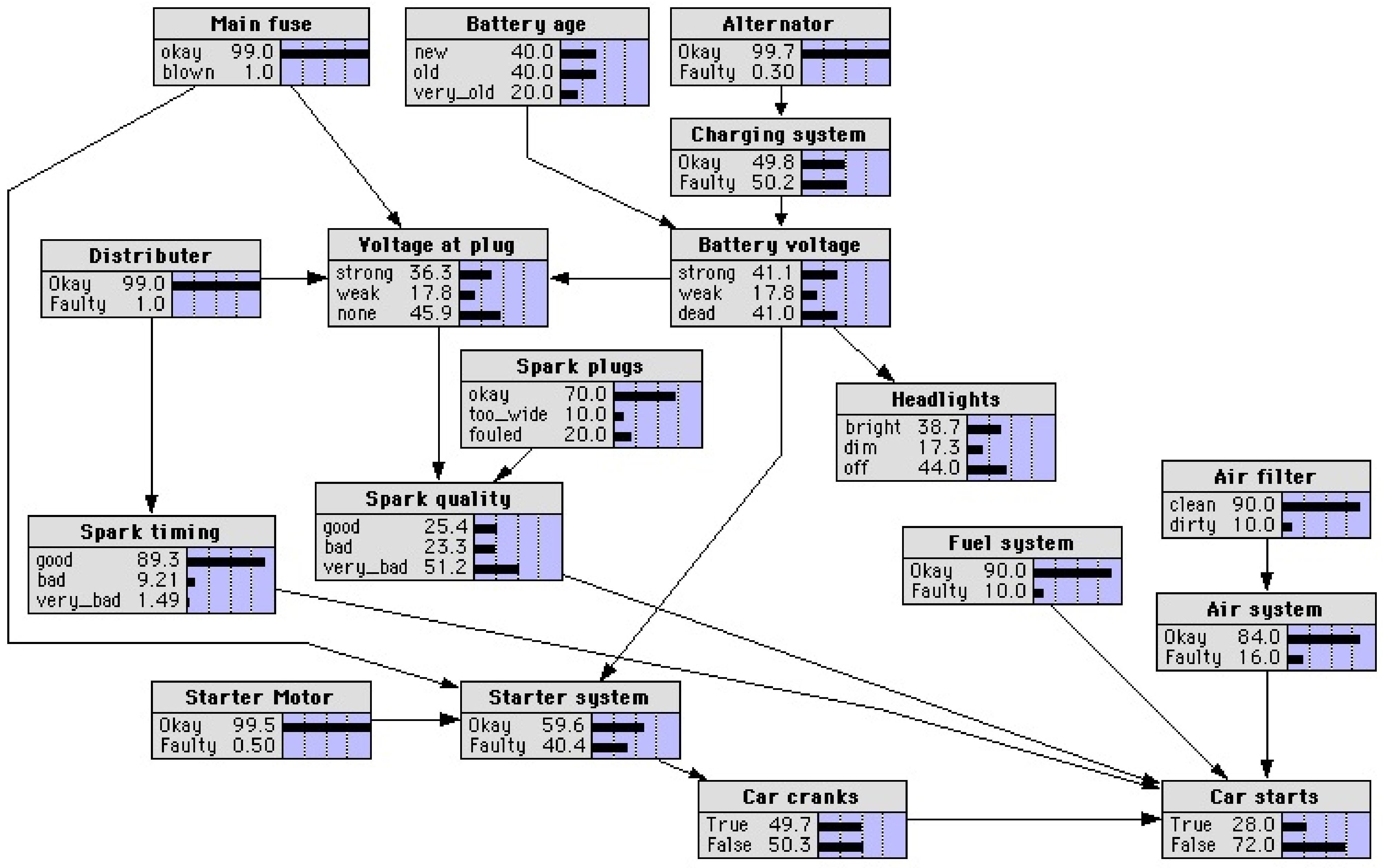
The second system, denoted
, is the “CAR_DIAGNOSIS_2” network from the library of benchmark BN made available by Norsys (
www.norsys.com/netlib/CarDiagnosis2.dnet). The system represents a network for diagnosing a car that does not start, based on spark plugs, headlights, main fuse, etc. It contains 18 nodes. From these nodes, seven nodes are health nodes (namely, the nodes labeled Main fuse, Alternator, Distributer, Starter motor, Air filter, Spark plugs, and Battery age).
Figure 3 shows the graphical representation of
.
Unfortunately, we did not have real data for the above systems from which to generate survival curves. The modeling of the components survival curves will be discussed in the next sections.
6.2. Diagnosis Experiments
In this set of experiments we evaluated the performance of the troubleshooting algorithm that uses survival functions to better guide its sensing actions (
Section 3.2). For this set of experiments we used a standard exponential curve for the survival function (defined earlier in this paper and illustrated in
Figure 1) with
. We tried several values of
. All values pointed on the same trends in the results, but with
we could see the trends clearly.
We compared the performances of four TAs: (1) random, which chooses randomly which component to sense, (2) BN-based, which chooses to sense the component most likely to be faulty according to the BN, (3) survival-based, which chooses to sense the component most likely to be faulty according to its survival curve and age, and (4) hybrid, which chooses to sense the component most likely to be faulty taking into consideration both BN and survival curve, as proposed in
Section 3.2. The performance of a TA was measured by the troubleshooting costs incurred until the system was fixed. Since we only considered single fault scenarios, we omitted the cost of the single repair action performed in each of these experiments, as all algorithms had to spend this cost in order to fix the system.
We generated random TP instances with a single faulty health node as follows.
First, we set the values of the control nodes randomly, according to their priors.
Then, the age of each component was sampled uniformly in the interval , where and are parameters.
Then, the conditional probability table of every health node was modified to take into account the survival curve, as mentioned in
Section 3.2; i.e., we replaced the prior probability for a component to be healthy with the value corresponding to its survival curve (
).
Next, we computed the marginal probability of each component to be faulty in this modified BN, and chose a single component to be faulty according to these computed probabilities.
Finally, we used the BN to sample values for all remaining observed nodes (the sensor nodes). A subset of these sensor nodes’ values was revealed to the DA.
The value of the was set to 0.3 (as for , with this value, we could show the impact of the other parameters the best). We examined the effects of the following parameters on the performances of the different TAs: (1) The parameter. (2) The revealed sensors parameter—this is the number of sensor node values revealed to the DA.
Results of the Diagnosis Experiments
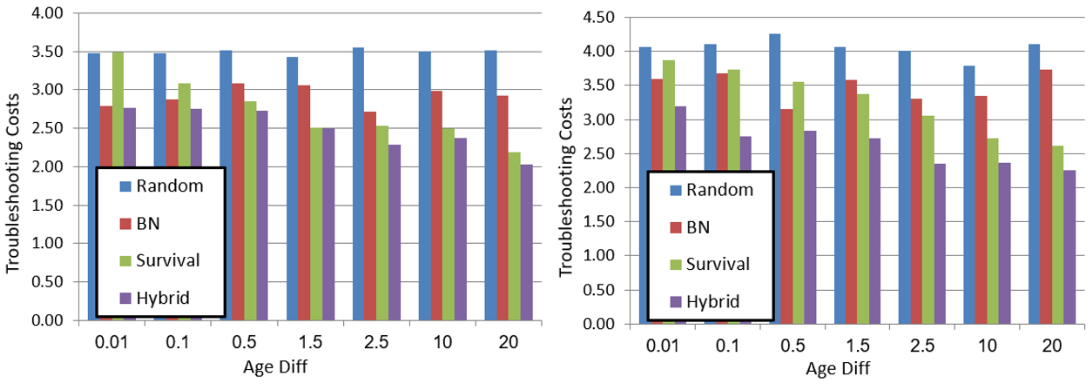
The plots in
Figure 4 show the average troubleshooting costs (
y-axis) for different values
(
x-axis), for each of the algorithms. The left plot shows the results for the
system and the right plot shows the results for
. All results were averaged over 50 instances.
Several trends can be observed. First, the proposed hybrid TA outperforms all baseline TAs, thereby demonstrating the importance of considering both survival curves and MBD. For example, in system
(
Figure 4 right) with an
, hybrid saves
troubleshooting costs compared to BN, and is slightly better than survival. Additionally, for
hybrid saves
compared to survival.
Second, the performance of survival improves as
grows. For example, in system
(
Figure 4 left) for
, the costs of survival and random are the same, but for
survival outperforms random. The reason for this is that increasing
means components’ ages differ more, and thus considering it is more valuable. When
is minimal, all components have approximately the same age, and thus using the survival curve to distinguish between them is similar to random. BN is better in this setting, since we provide it with some evidence—the values of some sensor nodes.
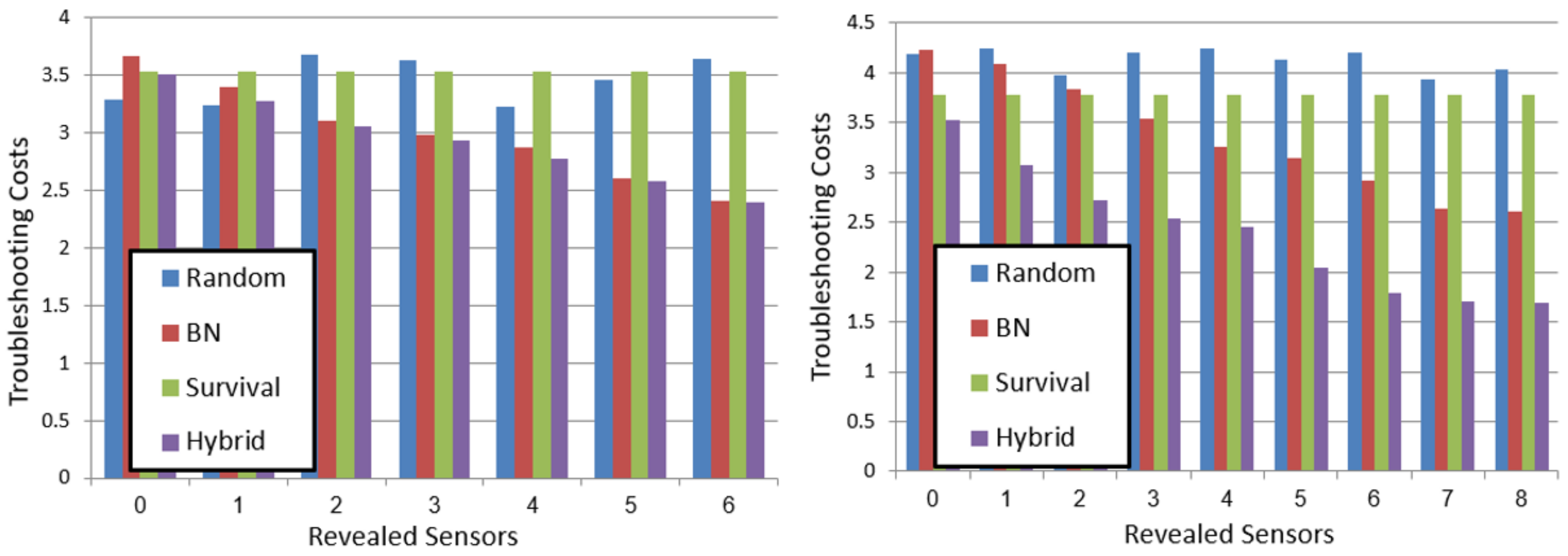
We also experimented with different numbers of revealed nodes.
Figure 5 shows the troubleshooting costs (
y-axis) for different values of revealed sensors on system
(left) and system
(right) with
parameter fixed to 0.5. As expected, revealing more nodes improves the performance of both BN and hybrid. Thus, in some settings of
and number of revealed sensors, BN is better than survival, and in others survival is better than BN. However, for almost all values of both parameters, hybrid is equal to or better than both. Thus, in conclusion, our results demonstrate that hybrid is more robust than both survival and BN across all varied parameters.
6.3. Long-Term Experiments
Next, we present experiments that evaluated the performances of the AT algorithms we proposed for solving the anticipatory troubleshooting dilemmas described in
Section 4.
6.3.1. Experimental Setup
Algorithm 2 describes how we realistically simulated the faults for the long-term experiment, based on the survival curves. First, we sampled for every component a failure time according to its survival curve. Then, a troubleshooting problem was created for the component
with the earliest failure time (line 2), and we invoked an AT algorithm to choose whether
C needs to be fixed or replaced (line 2). The age and survival curve of
C were then updated according to the chosen repair action. Next, we sampled new failure time for the component that had been repaired. Then, we invoked again an AT algorithm to choose whether there is a healthy component that should be replaced (line 2). If there were such components, their ages and failure times were updated accordingly. This process continued until the failure time of that component exceeded
. Then, we returned all costs incurred throughout the experiment.
affects the depth of the MDP; therefore, in our experiments we set
to 28, to enable the MDP algorithms to run in a reasonable time.
| Algorithm 2: Long-term simulation algorithm. |
 |
Note that we did not consider in these experiments the costs incurred due to sensing action. This is because in the long-term experiments we focus on how the evaluated algorithms solve the fix–replace and replace-healthy dilemmas. Thus, we measure only the cost incurred by repair actions ( and ) and the overhead cost ().
Evaluated Algorithms: In the experiments we compared the following algorithms to solve the fix–replace and replace-healthy dilemmas:
Always fix (AF), in which all faulty components are repaired using the Fix action.
Always replace (AR), in which all faulty components are repaired using the Replace action.
DR1, in which
DR1 (
Section 5.1) is used to choose the appropriate repair action.
N-, our MDP-based solver for solving only the fix–replace dilemma. It uses the
, as described in
Section 5.2.1, where
N stands for the level of granularity in the MDP.
N-, our MDP-based solver that considers both dilemmas, as described in Algorithm 1 in
Section 5.2.3, where
N stands for the levels of granularity in the MDPs.
Independent variables: We examined the effects of the following three independent variables on the performance of the different AT algorithms:
Punish factor. The punish factor parameter
p controls the difference between the
AfterFix curve and the regular survival curve. We did this by computing the
AfterFix as follows:
This
AfterFix curve holds the intuitive requirement that a replaced component is expected to survive longer than a fixed component. The parameter
p is designed to control the difference between the original and the
AfterFix curves. We refer to
p as the punish factor and set it in our experiments to values in the range of
.
Figure 6, for example, shows the survival curves of a new component and a fixed component that was fixed with a punish factor of 1.7. We set
in Equation (
7) as a fixed parameter. A greater value of
b biased the results to always replace policy, since it was not worthwhile to fix components.
Cost ratio. This is the ratio between and . The range of cost ratio values we experimented with was guided by the idea that the fix–replace ratio would be higher than 1 because usually replacing is more expensive than fixing a component.
Overhead ratio. This is the ratio between and . Recall that this cost is incurred whenever the system fails; this variable is relevant only for the replace-healthy dilemma.
The expected impact of each of these variables is as follows:
Higher punish factor means that fixing a component makes it more prone to error, so we expect an intelligent AT algorithm to replace components more often.
Similarly, a lower cost ratio means replacing a component is not much more expensive than fixing it, so we expect an intelligent AT to replace components more often.
Higher overhead ratio means it is more favorable to replace healthy components and save the expensive overhead.
The results reported below corroborated these expected impacts of our independent variables.
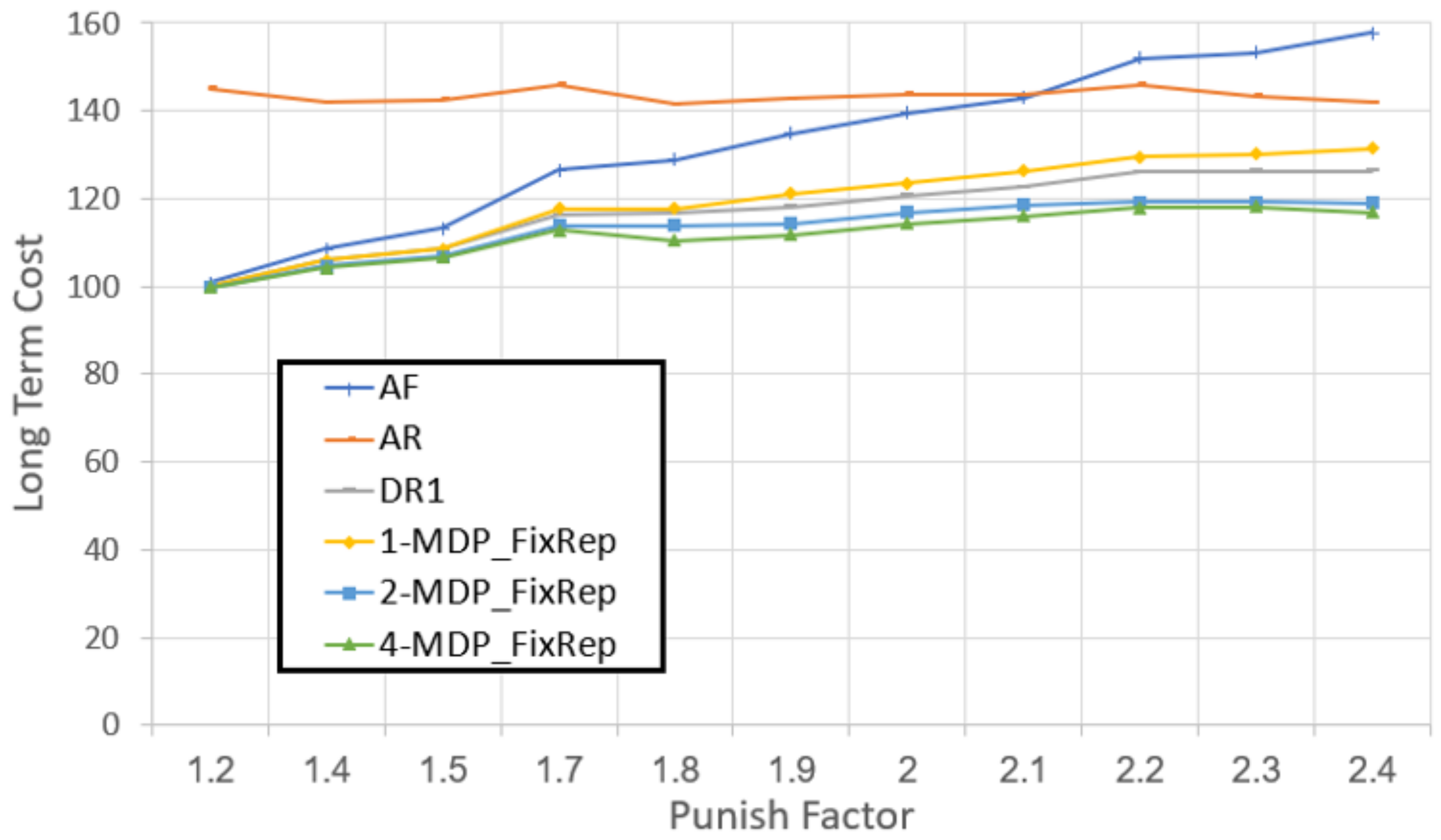
6.3.2. Results: Fix–Replace Dilemma
In the first set of experiments, we focused on the fix–replace dilemma, and thus we compared the baselines always-repair (AR) and always-fix (AF) with DR1 and N-.
Figure 7 presents the long-term costs (y-axis) as a function of the punish factor. As expected, using the
N- algorithm reduces the total troubleshooting cost. Moreover, the greater the granularity level (
N), the lower the costs are, since the MDP’s depth of the lookahead is greater and thus it is closer to find an optimal solution. Nevertheless, increasing
N beyond a certain value does not provide significant advantage in terms of long-term troubleshooting costs. In fact, in our experiments it was never worthwhile to use
N that was greater than 4.
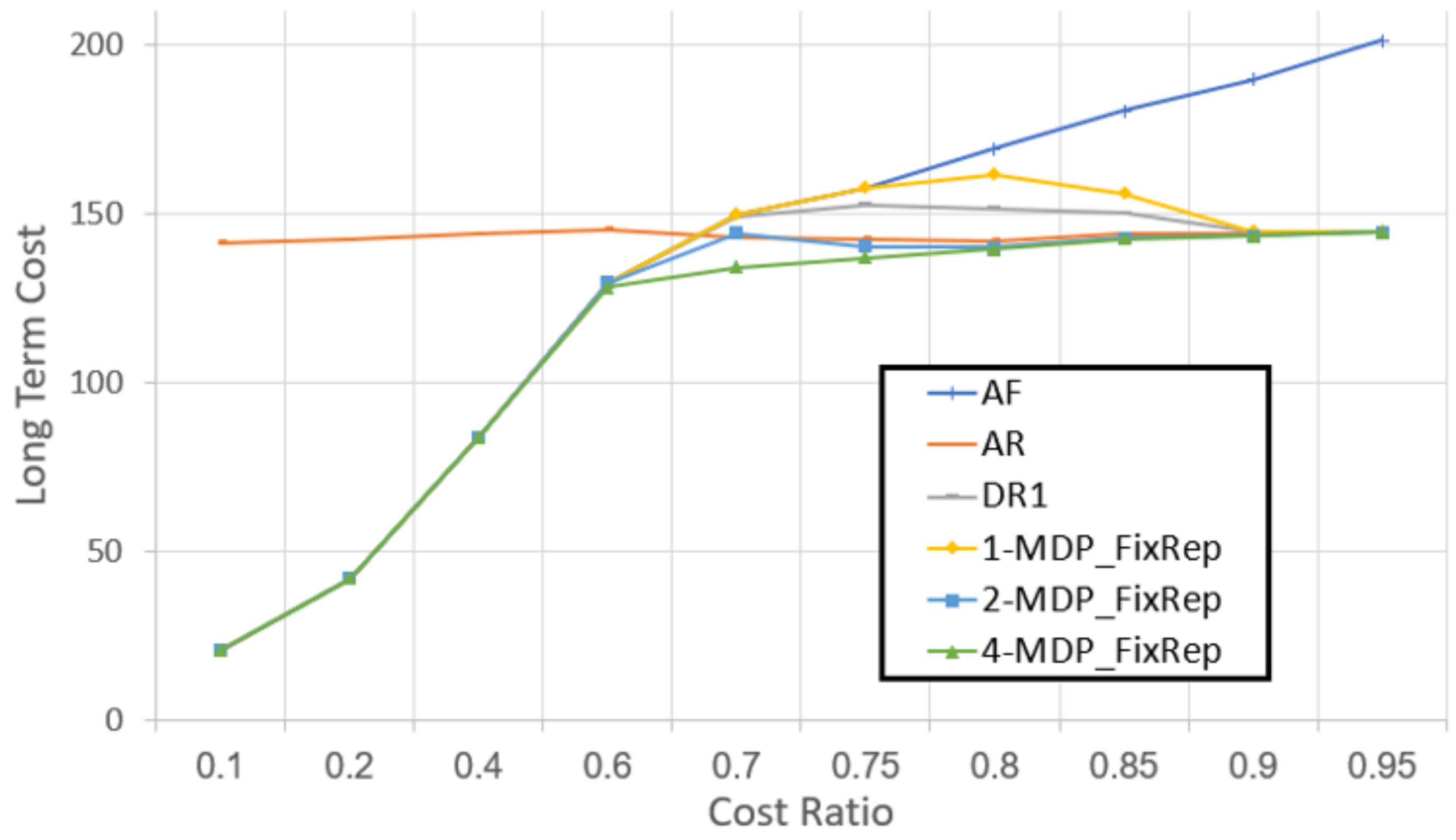
Figure 8 presents the long-term costs as a function of the cost ratio (the ratio between replacing and fixing costs). When the cost ratio is small, fixing is significantly cheaper than replacing, and thus the AF algorithm performed best. On the other hand, when the ratio is high, there is a small difference between the cost of fixing and replacing, but a new component is less likely to fail than a used component, and thus always-repair performs best. In both cases the
N- algorithm achieves the same cost as fixing for small ratio and as replacing for high ratio. In between, the
N- algorithm significantly reduces the cost compared to the baseline algorithms and the
DR1 algorithm.
6.3.3. Replace-Healthy Dilemma
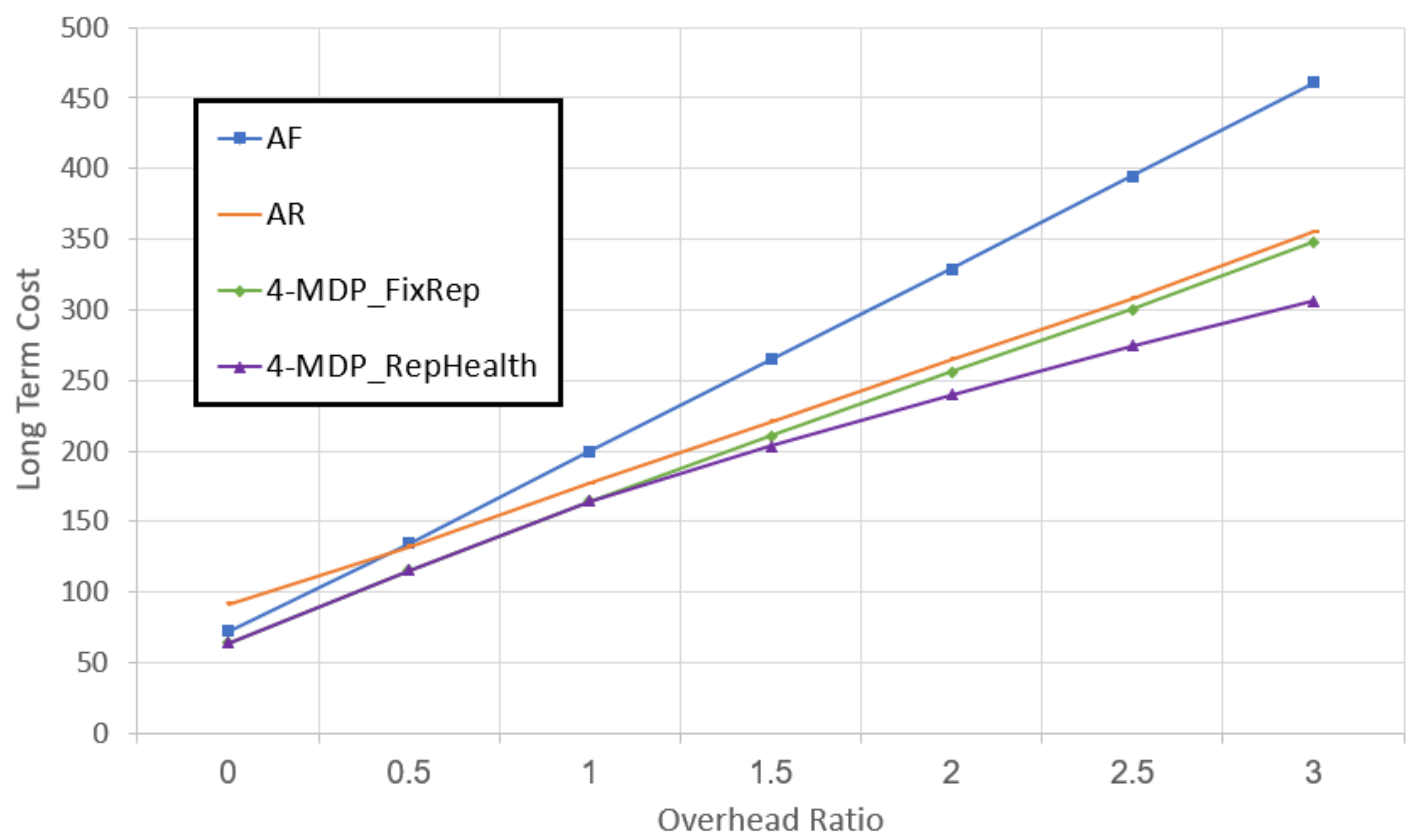
In the second set of experiments we analyzed the benefit of using our MDP-based solver to solve the replace-healthy dilemma. To that end, we compared N- to N-, both with , and to AF and AR.
Figure 9 shows the long-term troubleshooting costs (
y-axis) as a function of the overhead ratio (the ratio between
and
). The results show clearly that using
N- algorithm, which considers replacing healthy components, reduces the long-term troubleshooting costs. Additionally, the larger the overhead ratio, the bigger the benefit of
N-. As a side note, observe that as the overhead ratio gets higher, the
method becomes worse in relation to the other approaches, since solving every TP that arises becomes more expensive.
6.3.4. Discussion
The results above show the benefits of using our AT algorithm. However, there are cases where using AT algorithms is not beneficial. For example, when the cost of replacing is much more expensive than the cost of fixing, then it is clear from the results that always-fix policy keeps the long-term costs the lowest. Similarly, when the gap between the costs is very small, always-replace is the best policy. In between, our AT algorithms are beneficial. Thus, to save computational resources of the MDP-based methods, it may be worthwhile recognizing in advance the cases where always-replace or always-fix methods are dominant.
In addition, there are cases where it is never worthwhile to replace a healthy component. An obvious setting where this occurs is when the overhead cost is close to the cost of replacing. Another setting when replacing a healthy component is useless is when the component’s age has no effect on the probability that it will survive more time. That is, the probability that a component that has survived up to time t will fail before time is equal to the probability that a new component will fail before time . This occurs when the conditional probability of a component to survive more time given that it survived up to time t is equal to the unconditional probability that it will survive more time. That means the probability of failure is the same in every time interval, no matter the age of the component. Such distributions are known as "memoryless" probability distributions. An example of such a distribution is the distribution with the parameter b equal to 1 (known as exponential distribution). We experimented with this setting, and as expected, observed that there is no difference between a regular N- solver and an N- solver.
7. Related Work
There are several lines of work that are related to this research. We discuss them below. Probing and testing are well-studied diagnostic actions that are often part of the troubleshooting process. Intuitively, one would like to seek for the most informative observations and actions while doing the troubleshooting process. Probes enable one to observe the outputs of internal components, and tests enable further information, such as observing system output. Placing probes and performing tests can be very expensive. The basic idea is that not all probing and test choices are equal. Using this technique requires considerations, such as probe placement and which tests to choose. Those aspects have been studied over the years, and are also known as sequential diagnosis [
17,
22,
26,
27,
28]. Most works use techniques such as greedy heuristics and information gain; e.g., measuring the amount of information that observation
Y tells us about the diagnosis state
X. Some researchers present locally optimal solutions that run in linear time [
28,
29,
30]. Rodler [
29] proposes to use active learning techniques in order to achieve a nearly optimal sequence of queries. It should be noted that there are techniques that concentrate on saving system tests (e.g., a test that shows whether the system returned to its healthy state) and therefore consider batch repair in a period of time [
6,
31] rather than fix one component in each iteration [
3].
Many papers on automated troubleshooting are based on the seminal work of Heckerman et al. [
3] on decision theoretic troubleshooting (DTT). Our paper can be viewed as a generalization of DTT by taking prognosis into consideration. A decision theoretic approach integrates planning and diagnosis to a real-world troubleshooting application [
32,
33]. In their setting, a sequence of actions may be needed to perform repairs. For example, a vehicle may need to be disassembled to gain access to its internal parts. To address this problem, they use a Bayesian network for diagnosis and the AO* algorithm [
34] as the planner.
Friedrich and Nedjl [
35] propose a troubleshooting algorithm aimed at minimizing the breakdown costs, a concept that corresponds roughly to a penalty incurred for every faulty output in the system and for every time step until the system is fixed. Hakan and Jonas [
32] consider future repair actions using expected cost of repair and heuristic functions. They use a Bayesian network as the MBD and update the current belief state after each iteration. McNaught and Zagorecki [
36] also used two "repair" actions, but they do not use the prognostic information to decide which repair action to perform. Additionally, they did not use survival curves, but rather a dynamic Bayesian network which was unfolded to take time into consideration.
The novelty of our work is three-fold. First, none of these previous works incorporated prognosis estimates into the troubleshooting algorithm (as we did in
Section 3.2). Second, none of these previous works integrated prognosis estimates into a troubleshooting algorithm that aims at improving decision making when repairing the current fault, as we did. Finally, none of these works considered the dilemmas we present in this paper. Our anticipatory troubleshooting model and algorithm directly attempt to minimize costs incurred due to current and future failures through considering which repair action to take in each time step. Our goal is to minimize repair costs incurred through the lifetime of the system until a time threshold
T is reached.
A related line of work is in prognostics, where diagnostic information is used to provide more accurate remaining useful life estimations [
37,
38,
39]. In this research we used survival functions to improve the expected costs of repairing future system failures. There are many research fields where researchers use survival analysis to estimate the life time of an item or entity. For example, in electricity it is necessary to predict remaining battery life time [
40], and in chemistry it is required to predict failure scenarios of a nuclear system [
41]. Previous work showed how survival functions can be learned automatically from real data [
2,
41,
42,
43], or by deep learning methods [
44]. Alternatively, survival functions can be obtained from physical models.
While prognosis has been discussed considering troubleshooting, we are not aware of prior work that integrated survival functions, or any remaining useful life estimates, to minimize maintenance costs over time. Intelligently considering future costs raises many challenges that have not been addressed by prior work, such as fix faulty components rather than repairing them or replacing healthy but fault-prone components.
8. Conclusions
In this work we have discussed the concept of anticipatory troubleshooting that aims to save troubleshooting costs over time. We have presented two dilemmas that an anticipatory troubleshooting agent may face: the fix–replace dilemma and the replace-healthy components dilemma. The former deals with the question of which repair action to use to repair a given faulty component and the latter deals with the question of which currently healthy components to repair now in order to save future system failures. We solved both dilemmas by modeling them as a single MDP problem. Additionally, we have proposed a simple heuristic rule that solves the fix–replace dilemma. Key in this modeling is the use of survival functions to estimate the likelihood of future failures. We demonstrated the benefit of our approach experimentally, showing that our MDP-based solver can reduce the long-term troubleshooting costs. We have also proposed a way to improve the diagnosis phase by integrating diagnoses and prognoses that aim to reduce troubleshooting costs.
Our work opens up the possibility of future research in some directions. One such direction is to relax our assumption that components fail independently. While commonly used, this assumption does not hold in some settings. Thus, proposing an anticipatory troubleshooting algorithm that considers the relationships between components’ failures has the potential to be more effective. The challenge is how to relax this independence assumption while keeping the solution tractable. Similarly, we limited our discussion to the single-fault case, where only a single fault can occur in a time. This makes the MDP simpler and manageable. To extend our approach to multiple-fault scenarios, we will need to extend the MDP state space so that more than one fault can occur in a given time step. This will make the MDP state space exponentially larger, suggesting that intelligent methods will be needed to make it scale. Similarly, having more than two possible repair actions is also challenging, increasing the branching factor of the MDP state space. Another important direction for future work is to implement an anticipatory troubleshooting algorithm in a real-life system.


