Article

Chaotic Discrete Fractional-Order Food Chain Model and Hybrid Image Encryption Scheme Application

by
Sameh Askar
1,2,*,
Abdulrahman Al-khedhairi
1,
Amr Elsonbaty
3 and
Abdelalim Elsadany
4
1
Department of Statistics and Operations Research, College of Science, King Saud University, P.O. Box 2455, Riyadh 11451, Saudi Arabia
2
Department of Mathematics, Faculty of Science, Mansoura University, Mansoura 35516, Egypt
3
Department of Engineering Mathematics and Physics, Faculty of Engineering, Mansoura University, Mansoura 35516, Egypt
4
Basic Science Department, Faculty of Computers and Informatics, Suez Canal University, Ismailia 41522, Egypt
*
Author to whom correspondence should be addressed.
Symmetry 2021, 13(2), 161; https://doi.org/10.3390/sym13020161
Submission received: 27 December 2020 / Revised: 10 January 2021 / Accepted: 18 January 2021 / Published: 21 January 2021
(This article belongs to the Special Issue Bifurcation and Chaos in Fractional-Order Systems)

Abstract

:
Using the discrete fractional calculus, a novel discrete fractional-order food chain model for the case of strong pressure on preys map is proposed. Dynamical behaviors of the model involving stability analysis of its equilibrium points, bifurcation diagrams and phase portraits are investigated. It is demonstrated that the model can exhibit a variety of dynamical behaviors including stable steady states, periodic and quasiperiodic dynamics. Then, a hybrid encryption scheme based on chaotic behavior of the model along with elliptic curve key exchange scheme is proposed for colored plain images. The hybrid scheme combines the characteristics of noise-like chaotic dynamics of the map, including high sensitivity to values of parameters, with the advantages of reliable elliptic curves-based encryption systems. Security analysis assures the efficiency of the proposed algorithm and validates its robustness and efficiency against possible types of attacks.

1. Introduction

Fractional order differentiation and integration can be considered as a generalization of conventional integer order calculus to noninteger real or even complex valued orders. The history of fractional calculus has started about 300 years ago. Fractional calculus can be used to describe memory dependent behaviors and inherited properties of nonlinear systems. As a mathematical tool, it provides an extra degree of freedom to implement and interpret many real world systems with higher accuracy than the integer-order equivalent [1,2,3,4,5,6]. For example, most physical and engineering systems show complex behaviors such as nonlinear circuits, nanophotonics, viscous systems and laser systems. Compared to the integer-order differential equation, the memory effects are considered in the fractional-order differential equations and allow more accurate description of these natural phenomena [7]. One important aspect of dynamic systems is their chaotic behavior. A great deal of attention to this behavior has been paid in various areas of application where many fruitful results have been achieved over the past decades. For example, the authors of [8] updated Chua’s model to include elements of fractional order and demonstrated chaos and other nonlinear behaviors. Several continuous time chaotic fractional order models, such as the fractional-order Lorenz [9,10,11] and the Chen fractional-order systems [12,13,14], have been examined and employed in several interesting fields such as control of chaos [15,16,17], nonlinear circuits [18,19], chaos based encryption [20] and medical applications [21]. The analytical and numerical study of dynamic propagation of light beams in the fractional order Schrödinger equation with a harmonic potential have been presented in [22]. The dynamics in stochastic models of Gaussian-amplitude field, phase-diffusion and chaotic field in laser have been investigated in [23,24].
Although continuous-time fractional order models have been applied successfully many times to describe and understand some nonlinear phenomena which classical integer order models fail to deal with, it is found that a discretization problem is usually attached to the numerical solutions of continuous fractional models. In particular, the occurrence of different types of errors and the high computational costs limit the perfect utilization of these models. Therefore, the interest of mathematicians is directed to straightforward exploitation of discrete fractional calculus and fractional difference equations which are more appropriate and effective in mathematical modeling of systems with memory influences. Recently, the discrete fractional calculus field is rapidly developed where many new related applications are explored. The fractional-order logistic map has been studied by Wu and Baleanu [25] where unique bifurcation scenarios and chaotic dynamics were noticed compared to the whole-order system. Nonetheless, the initial values of iterations are not completely eliminated and thus the bifurcation diagram appeared non-refined and the estimated values of Lyapunov exponents may be inaccurate. Based on the fractional disparity, Wu and Baleanu also discussed the discrete fractional order versions of Sine map and Standard map [26]. Khennaoui et al. [27] subsequently produced the fractional-order Unified map, and Liu [28] and Shukla et al. [29] studied the fractional-order Henon map. Ji et al. [30] recently introduced a new Grunwald–Letnikov-based fractional-order logistic map which exhibits different properties from the above aforementioned maps.
Among the most attractive applications of chaotic dynamics, chaos-based cryptography is intended to utilize preferable features of chaotic behaviors to ensuring secure transmission of private data between legitimate sender and receiver. In particular, the key characteristics of these encryption systems are extreme sophistication and dimensionality of disorder implemented in these schemes, in addition to the efficient protection of fundamental information about encryption system from being extracted by any unauthorized attacker. There are several techniques which have been suggested to enhance security performance and chaotic dynamics of chaos-based encryption system, see for example [31,32,33,34,35]. In addition, chaotic discrete fractional systems have been investigated in [36,37,38,39,40,41] and further implemented in some efficient cryptosystem in [42,43,44,45,46,47,48].
Elliptic curves-based encryption systems are examples of reliable and efficient public key techniques which proved their advantages over the other like techniques such as DH, El-Gamal, RSA, etc. Thus, to build a superior cryptosystem, the aim of this paper was to merge the advantages of elliptic curve technique with the complicated noise-like dynamics of the current spontaneous chaotic system. More specifically, the complicated dynamics of the fractional-order map is combined with powerful elliptic curve key exchange scheme.
The paper is set out as follows. In Section 2, some preliminaries and mathematical principles are presented. In Section 3, the discrete fractional difference equations are employed for description of chaotic food chain model having non-overlapping generations and subject to intraspecific competition along with strong pressure on prey species. To the best of authors’ knowledge, this the is first time to employ discrete fractional calculus in mathematical modeling of food chains and investigate the influences of fractional order on the dynamics of the model. In Section 4, numerical simulations of the discrete fractional-order model are carried out. In Section 5, a proposed hybrid cryptosystem is introduced with input data in the form of colored images. Security performance of the proposed encryption scheme is investigated in Section 6 to validate its reliability and efficiency. Finally, the overall discussion and conclusion are concluded in Section 7.

2. Preliminaries

In order to overcome the difficulties that arise from dealing with continuous time fractional order system and efficiently capture the memory effects, discrete fractional calculus was introduced [46,47,48,49,50]. The studies of dynamic behaviors and applications of fractional delta difference models attracted increasing interest in the last decade, see [49,50,51,52,53,54] and references therein.
The sequence χ ( n ) is supposed to be given at isolated discrete times a which is described in terms of constant τ such that { τ , τ + 1 , τ + 2 ,…,} and χ : τ R . Moreover, let the difference operator be referred to as Δ , where Δ χ ( n ) = χ ( n + 1 ) χ ( n ) .
Definition 1.
The fractional sum of order α where α > 0 , is defined by [53]
Δ τ α χ ( t ) = 1 Γ ( α ) m = τ t α Γ ( t m ) Γ ( t m α + 1 ) χ ( m ) , t τ + α .
Definition 2.
The order α delta difference of Caputo-sense is given as [54]:
C Δ τ α χ ( t ) = Δ τ ( n α ) Δ n χ ( t ) = 1 Γ ( n α ) m = τ t ( n α ) Γ ( t m ) Γ ( t m n + α + 1 ) Δ n χ ( m ) , t τ + α , n = [ α ] + 1 .
Definition 3.
The order α fractional delta difference equation is defined as [55]:
C Δ τ α χ ( t ) = f ( t + α 1 , χ ( t + α 1 ) ) ,
where its associated discrete time integral is expressed as
χ ( t ) = χ 0 ( t ) + 1 Γ ( α ) m = τ + n α t α Γ ( t m ) Γ ( t m α + 1 ) f ( m + α 1 , χ ( m + α 1 ) ) , t τ + n .
Here, the initial value can be written as
χ 0 ( t ) = k = 0 n 1 Γ ( t τ + 1 ) k ! Γ ( t τ k + 1 ) Δ k χ ( t ) .
Theorem 1
([55]). The delta fractional difference equation
C Δ τ α x ( t ) = f ( t + α 1 , x ( t + α 1 ) ) Δ k x ( t ) = x k , n = n = [ α ] + 1 , k = 0 , 1 , , n 1
has the following equivalent discrete integral equation
x ( t ) = x 0 + 1 Γ ( α ) s = τ + n α t α ( t σ ( s ) ) ( α 1 ) f ( s + α 1 , x ( s + α 1 ) ) , t τ + n ,
such that
x 0 ( t ) = k = 0 m 1 ( t τ ) k k ! Δ k x ( τ ) .
Remark 1.
If τ = 0 , we rewrite discrete integral equation in the next numerical expression
x ( n ) = x 0 + 1 Γ ( α ) s = 1 n Γ ( n s + α ) Γ ( n s + 1 ) f ( x ( s 1 ) ) .
Theorem 2.
The conditions of asymptotic stability of zero equilibrium point to the next discrete fractional-order system
C Δ τ α X ( t ) = M X ( t + α 1 ) ,
where X ( t ) = ( x 1 ( t ) , x 2 ( t ) , , x n ( t ) ) T , 0 < α 1 , M R n × n and t τ + 1 α are
λ z C : z < ( 2 cos arg z π 2 α ) α ,   arg z > α π 2 ,
for every eigenvalues λ of the discrete fractional system.

3. Discrete-Time Fractional-Order Food Chain Model

Discrete-time dynamic systems are ideal to describe the population dynamics of non-overlapping organisms. It is well known that one of the basic population models is the Lotka–Volterra prey-predator model. Holling has introduced the study of more practical predator models since the groundbreaking theoretical works by Lotka [56] and Volterra [57] in the last century, proposing three types of functional responses for different species to model predation dynamics [58].
The discrete time models are known to exhibit more complicated dynamics than their counterpart continuous time models. For example, the chaotic behavior can be induced by the simple one-dimensional logistic map while only exponential growth or decaying of state variable can be observed in logistic differential equation. The main interest of mathematicians and scientists was focusing on continuous time models in mathematical biology and ecology for a long time. The capability of discrete time models to describe some cases of species dynamics efficiently brought them to light quite recently. In 2020, a novel discrete time novel food chain model was introduced [59] as the first discrete model to consider three interacting organisms, having non-overlapping generations, which is subjected to intraspecific competition and strong pressure on preys species. More specifically, we consider a prey population x predated by a first predator species y. The third species is the top predator z that predates on the first predator y and simultaneously interferes with the population growth of prey. The model proposed for studying these ecological interactions is represented by the following nonlinear discrete system [59]:
x n + 1 = a x n ( 1 x n y n z n ) , y n + 1 = b y n ( x n z n ) , z n + 1 = c y n z n .
For the function f ( n ) , the delta difference operator is defined by Δ f ( n ) = f ( n + 1 ) f ( n ) .
Based on previous assumptions, we get the following discrete fractional-order food chain model for (1):
C Δ τ α x n = a x n ( 1 x n y n z n ) x n , C Δ τ α y n = b y n ( x n z n ) y n , C Δ τ α z n = c y n z n z n .
The fixed points of system (2) satisfy
0 = a x n ( 1 x n y n z n ) x n , 0 = b y n ( x n z n ) y n , 0 = c y n z n z n .
By simple algebraic computations, we obtain four fixed points for the abo
E 0 = ( 0 , 0 , 0 ) , E 1 = ( a 1 a , 0 , 0 ) , E 2 = ( 1 b , 1 1 a 1 b , 0 ) , E 3 = ( 1 2 ( 1 1 a + 1 b 1 c ) , 1 c , 1 2 ( 1 1 a 1 b 1 c ) .
In the following subsection, the local stability of these fixed points are studied for model (2).

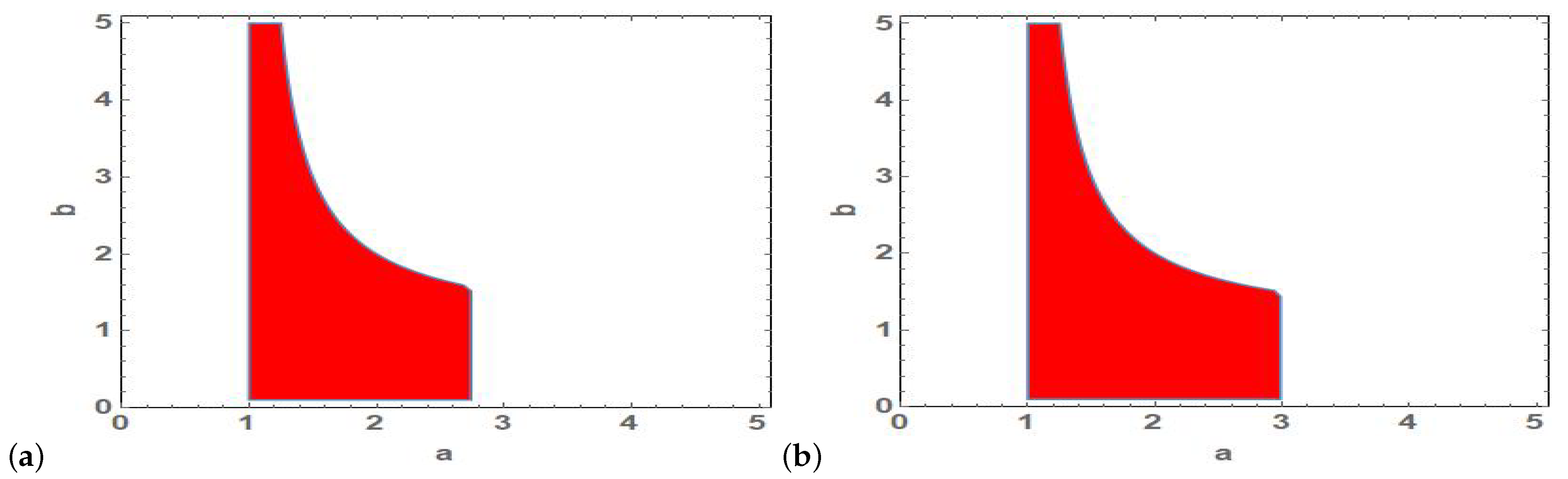
3.1. Stability of Fixed Points

The local stability analysis of the fixed points is established by studying the Jacobian matrix of system (1) at these fixed points. The system (2) can be linearized about any fixed point ( x * , y * , z * ) via computing its associated Jacobian matrix which takes the form
J = a ( 1 x * y * z * ) a x * 1 a x * a x * b y * 1 + b ( x * z * ) b y * 0 c z * 1 + c y * .
The characteristic equation of matrix J is computed and expressed in the form
λ 3 + ν 1 λ 2 + ν 2 λ + ν 3 = 0 ,
where, ν 1 = 2 a x * + a y * + a z * a b x * + b z * c y * + 3 , ν 2 = a b x * z * 2 a b x * 2 + a b x * + a b y * z * + a b z * 2 a b z * 2 a c x * y * a c y * z * a c y * 2 + a c y * + 4 a x * + 2 a y * + 2 a z * 2 a + b c x * y * 2 b x * + 2 b z * 2 c y * + 3 , ν 3 = 2 a b c x * y * z * + 2 a b c x * 2 y * a b c x * y * + a b x * z * 2 a b x * 2 + a b x * + a b y * z * + a b z * 2 a b z * 2 a c x * y * a c y * z * a c y * 2 + a c y * + 2 a x * + a y * + a z * a + b c x * y * b x * + b z * c y * + 1 .
Thus, the stability analysis of each fixed point is carried out as follows:

3.1.1. Stability Analysis of E 0

For this fixed point, it is found that the eigenvalues of J are given by
λ 1 , 2 = 1 , λ 3 = a 1 .
This implies that
λ 1 , 2 = 1 , A r g ( λ 1 , 2 ) = π , λ 3 = a 1 if a 1 1 a if a < 1 , A r g ( λ 3 ) = 0 if a 1 π if a < 1 .
Referring to the conditions of asymptotic stability of fixed points which are given in previous section, the fixed point E 0 is locally asymptotically stable if 0 < a < 1 . Figure 1 shows the stability region of fixed point E 0 in parameters’ plane (a, α ).

3.1.2. Stability Analysis of E 1

For this fixed point, it is found that the eigenvalues of J are given by
λ 1 = 1 , λ 2 = 1 a , λ 3 = 1 + b b a ,
that implies that
λ 1 = 1 , A r g ( λ 1 ) = π , λ 2 = a 1 if a > 1 1 a if a 1 , A r g ( λ 2 ) = π if a > 1 0 if a 1 , λ 3 = 1 + b b a if b 1 + b a 1 b + b a if b < 1 + b a , A r g ( λ 3 ) = 0 if b 1 + b a π if b < 1 + b a .
Referring to the conditions of asymptotic stability of model’s steady states which are given in the previous section, the fixed point E 1 satisfies local asymptotic stability in the red colored regions illustrated in Figure 2 which depends on the values of a , b and α .

3.1.3. Stability Analysis of E 2

For this fixed point, it is found that the eigenvalues of J are given by
λ 1 = a 2 a 2 4 a b 2 + 4 a b + 4 b 2 a 3 2 a 2 b , λ 2 = a 3 a 2 a 2 4 a b 2 + 4 a b + 4 b 2 2 a 2 b , λ 3 = a b c a b a c b c a b .
In order to find local asymptotic stability region in space of parameters of model (2), numerical evaluations of values of parameters which satisfy stability conditions can be used. In particular, Figure 3 shows examples of stability regions in ( a , b ) and ( a , c ) planes of parameters for distinct values of fractional order α .

3.1.4. Stability Analysis of E 3

First, this point takes values within the feasible space if the following condition is satisfied
1 a + 1 b + 1 c < 1 ,
which means that this condition should be examined along with the aforementioned stability conditions. For the fixed point E 3 , it is found that the eigenvalues of J have very complicated expressions which renders the numerical investigations of asymptotic stability region in space of parameters of model (2). In Figure 4, regions of occurrence of fixed point E 3 in addition to colored stability regions in ( a , b ) and ( a , c ) planes of parameters at distinct values of α are depicted.

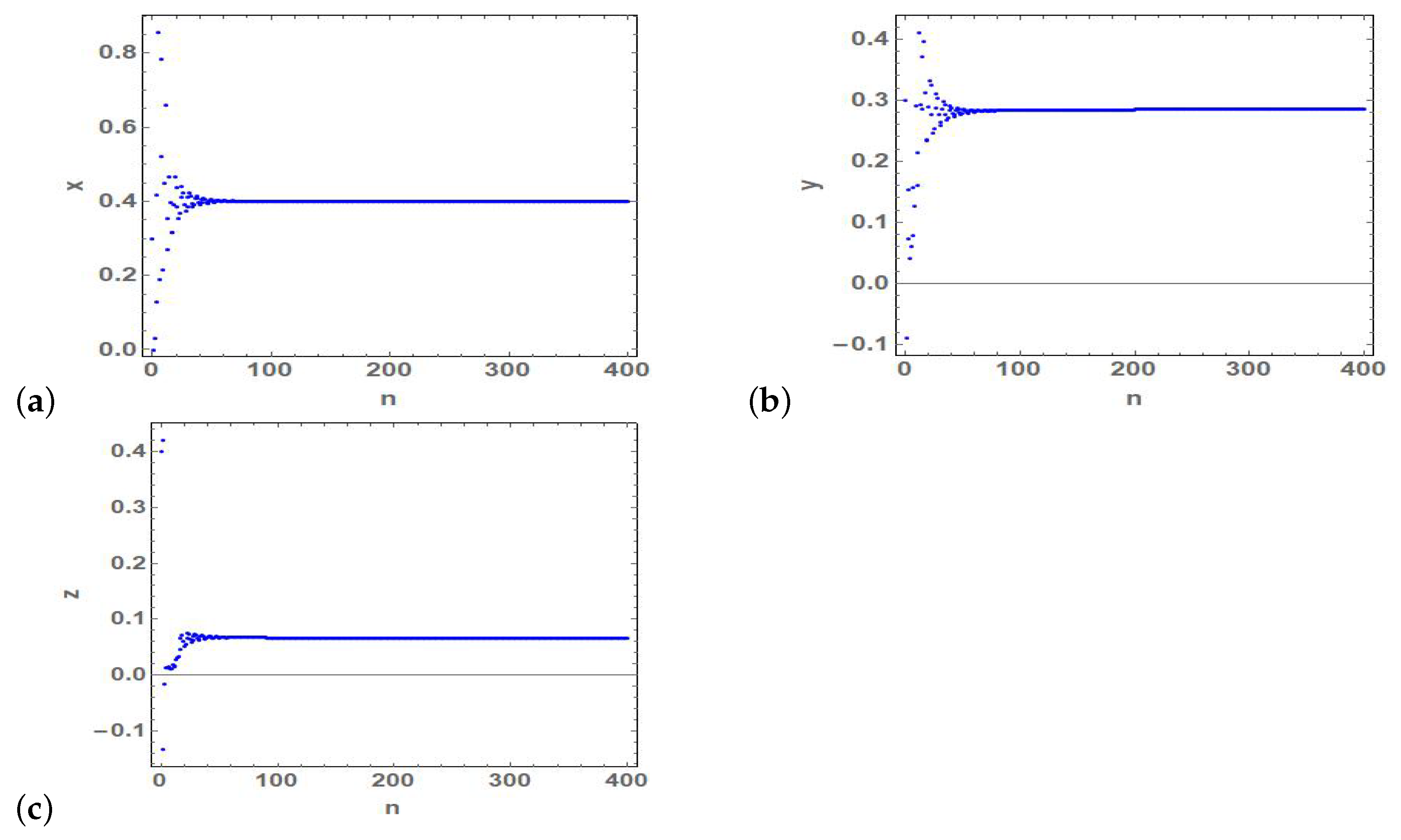
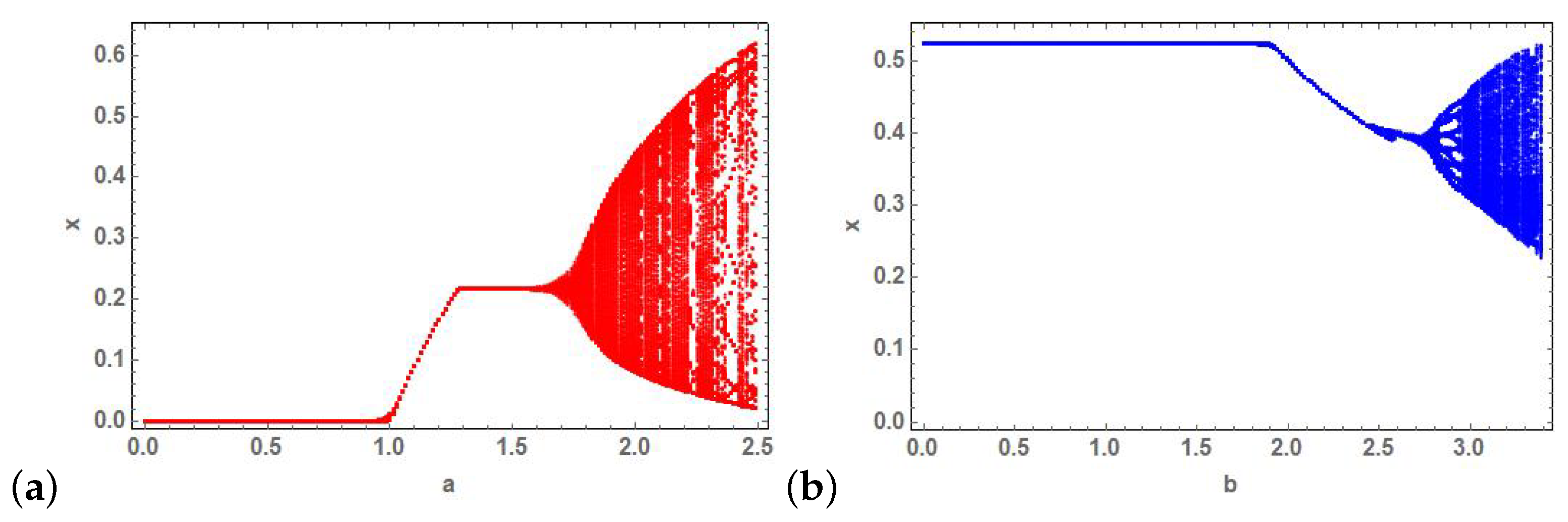
4. Numerical Simulations

In this section, results of numerical simulations are shown for integer order model (1) and fractional order model (2). The phase portraits and bifurcation diagrams are employed to determine variation in dynamical behaviors of the two models in terms of variations in parameters in the models. In the following simulations, system (2) is used in the following form:
x ( n ) = x ( 0 ) + 1 Γ ( α ) s = 1 n Γ ( n s + α ) Γ ( n s + 1 ) a x s 1 ( 1 1 a x s 1 y s 1 z s 1 ) , y ( n ) = y ( 0 ) + 1 Γ ( α ) s = 1 n Γ ( n s + α ) Γ ( n s + 1 ) b y n 1 ( x s 1 z s 1 1 b ) , z ( n ) = z ( 0 ) + 1 Γ ( α ) s = 1 n Γ ( n s + α ) Γ ( n s + 1 ) z n 1 ( c y s 1 1 ) .
Firstly, the aforementioned conditions of stability of fixed points of model (2) are verified. In particular, the values of parameters which yield a stable fixed point E 0 is from Figure 1 and the associated time series outputs of model (2) are presented in Figure 5 and confirm theoretical results.
Similarly, the values of parameters which correspond to stable fixed points E 1 , E 2 and E 3 are presented from Figure 2, Figure 3 and Figure 4, respectively. Furthermore, the output time series which are illustrated in Figure 6, Figure 7 and Figure 8 are, respectively, verify stability conditions of fixed points E 1 , E 2 and E 3 . In Figure 6, time series of state variables of (2) show stability of fixed point E 1 at a = 2 , b = 1 , c = 1 and α = 0.9 .
Secondly, the bifurcation diagrams are employed to overview the influences of parameter’s variations on dynamical behaviors of models (1) and (2). The case of integer order model (1) is presented in Figure 9 where the effects of variations in parameters a and b are shown. The influences of fractional order α along with other parameters are depicted in Figure 10.
Finally, some selected examples of phase portraits of the two models (1) and (2) are shown in Figure 11.
It is obvious that increasing predation rate of predators on the prey, the mode can exhibit chaotic dynamics. In particular, the model undergoes a stable Neimarck–Sacker bifurcation followed by period-doubling bifurcations till chaos behavior starts arises.

5. Hybrid Image Encryption Scheme

In this section, we propose an encryption scheme that combines elliptic curve key exchange technique with chaotic output of a three-dimensional mapping. Numerical simulations on different color images are used to validate the efficiency of the scheme against differential, statistical in addition to brute-force attacks.
Input: Assume that a colored plain image with size of m × n pixels is given. Then, three values of color components are associated to each pixel in the image. These color components are red, green and blue such that for each pixel with position ( i , j ) , let R ( i , j ) , G ( i , j ) and B ( i , j ) refer to the values of red, green and blue color components, respectively. Typically, they take the range [ 0 : 255 ] . In addition, assume that the reading of internal clock of encrypting machine is given by T * at the moment when encryption session starts.
Public Keys: Pick one family of elliptic curves standardized by the NIST, its associated group generator and parameters are considered as public keys of the suggested scheme. In the next numerical experiments, we adopt the P-192 curve groups of the following form
y 2 = x 3 3 x + β ,
where
G = {602 046 282 375 688 656 758 213 480 587 526 111 916 698 976 636 884 684 818, 174 050 332 293 622 031 404 857 552 280 219 410 364 023 488 927 386 650 641},
β = 2 455 155 546 008 943 817 740 293 915 197 451 784 769 108 058 161 191 238 065,
q = 6 277 101 735 386 680 763 835 789 423 207 666 416 083 908 700 390 324 961 279, refer to the generator of the group, the parameter of the curve and the modulus of finite field, respectively.
Secret Keys: Secret keys are known only to both or one of authentic sides of secure communications link. They are listed in following points:
(1) The initial values of parameters in model (2) which are denoted by a 0 , b 0 ,   c 0 , and α 0 .
(2) Private key of transmitter side, i.e., P t .
(3) Private key held by the receiver, i.e., P r .
(4) Three arbitrary chosen real number μ i , i = 1 , 2 , 3 .
(5) The value of T * .
Encryption/Decryption Process:
(1) Evaluate the following three perturbing values which depend on plain image
δ R = μ 1 ( m × n ) 2 i = 1 m j = 1 n R ( i , j ) + T * , δ G = μ 2 ( m × n ) 2 i = 1 m j = 1 n G ( i , j ) + T * , δ B = μ 3 ( m × n ) 2 i = 1 m j = 1 n B ( i , j ) + T * .
(2) Update the values of secret parameters according to one of the following rules
a = a 0 + δ R , b = b 0 + δ G , c = c 0 + δ B ,
a = a 0 + δ R , b = b 0 + δ B , c = c 0 + δ G ,
a = a 0 + δ G , b = b 0 + δ R , c = c 0 + δ B ,
a = a 0 + δ G , b = b 0 + δ B , c = c 0 + δ R ,
a = a 0 + δ B , b = b 0 + δ G , c = c 0 + δ R ,
a = a 0 + δ B , b = b 0 + δ R , c = c 0 + δ G .
(3) Apply the updated values of parameters to simulate the model (2) discarding any transient nonchaotic dynamics. The resulting chaotic time series of lengths m × n + 2 × max { m , n } are to be used in the next steps.
(4) Construct the following encrypting sequences
S R r = m o d ( I n t e g e r P a r t [ x i × 10 10 ] , m ) ,
S G r = m o d ( I n t e g e r P a r t [ y i × 10 10 ] , m ) ,
S B r = m o d ( I n t e g e r P a r t [ z i × 10 10 ] , m ) , i = 1 , 2 , , m .
S R c = m o d ( I n t e g e r P a r t [ x i × 10 10 ] , n ) ,
S G c = m o d ( I n t e g e r P a r t [ y i × 10 10 ] , n ) ,
S B c = m o d ( I n t e g e r P a r t [ z i × 10 10 ] , n ) , i = m + 1 , m + 2 , , m + n .
S 1 = m o d ( I n t e g e r P a r t [ x i × 10 10 ] , 256 ) ,
S 2 = m o d ( I n t e g e r P a r t [ y i × 10 10 ] , 256 ) ,
S 3 = m o d ( I n t e g e r P a r t [ z i × 10 10 ] , 256 ) , i = 1 + 2 × max { m , n } , 2 + 2 × max { m , n } , , m × n + 2 × max { m , n } .
(5) The values of S R r , S G r , S B r , S R c , S G c and S B c are arranged in an ascending order to formulate six confusion vectors. Hence, the rows of original matrix of pixels are permuted such that the red components are scrambled according to components of S R r whereas green and blue values in each row are confused by S G r and S B r orders, respectively. By the same way, the columns in the original image are scrambled by utilizing S R c , S G c and S B c .
(6) The plain image is reshaped into three vectors each of which has m × n values. These vectors involve the separate values of pixels’ color intensity. They are referred as I 1 , I 2 and I 3 .
(7) The bitwise XOR operations are carried out between vectors S 1 , S 2 , S 3 and I 1 , I 2 , I 3 such that the three encrypted components of cipher images are computed as
I e n c R = I 1 S 1 , I e n c G = I 2 S 2 , I e n c B = I 3 S 3 .
(8) The elliptic curve key exchange technique in the sense of Diffie–Hellman is adopted such that the sender side publishes P t G whereas the receiver side publishes P r G . Thus, the sender and receiver will agree on a common symmetric key P t P r G = P r P t G .
(9) Three perturbation values δ t , t = R , G , B are encoded using the shared secret key. More specifically, El-Gamal scheme can be applied [60] at this step.
(10) The shared secret keys and similar numerical precision settings at both sides, imply that identical versions of chaotic sequence S 1 , S 2 and S 3 are generated at the receiver part.
(11) The transmitted ciphered image is deciphered through the aforementioned bitwise XOR operations.
(12) Finally, the deciphered vectors are reshaped to restore the original plain image.

6. Security Analysis of the Proposed Scheme

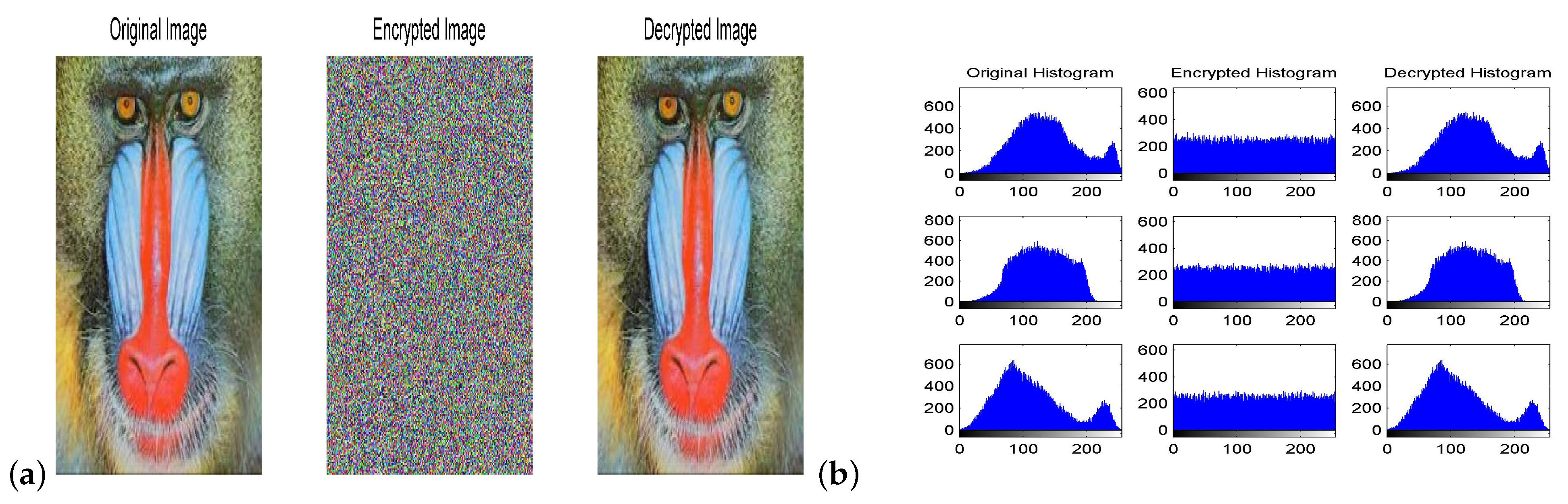
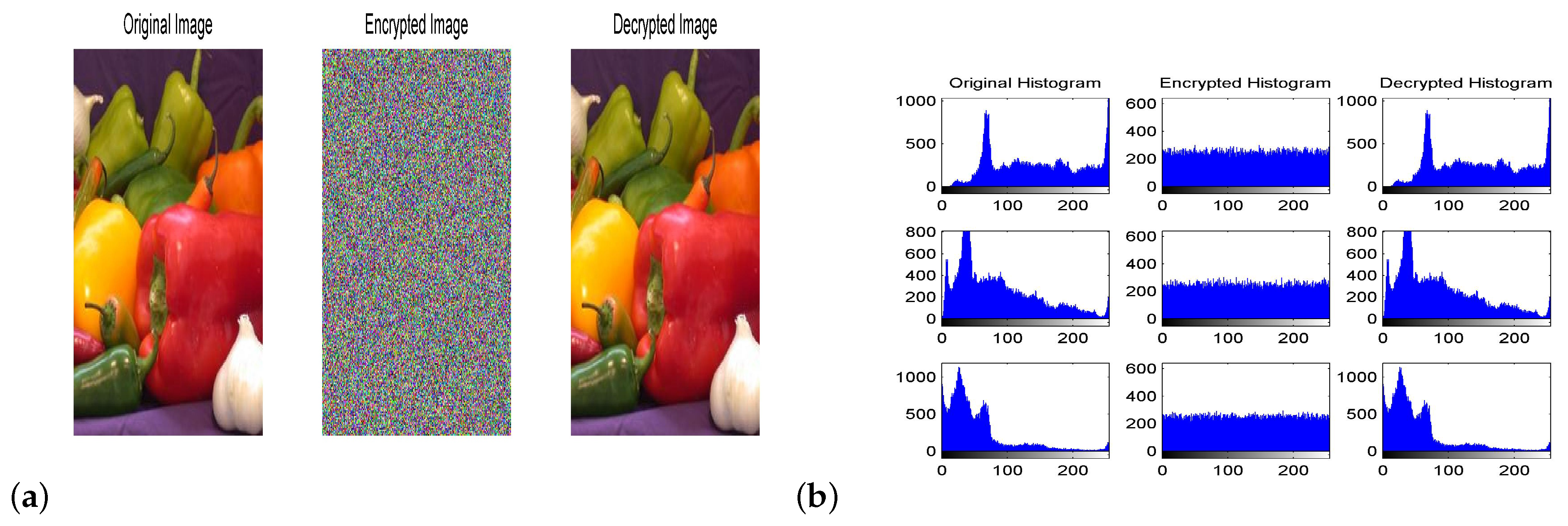
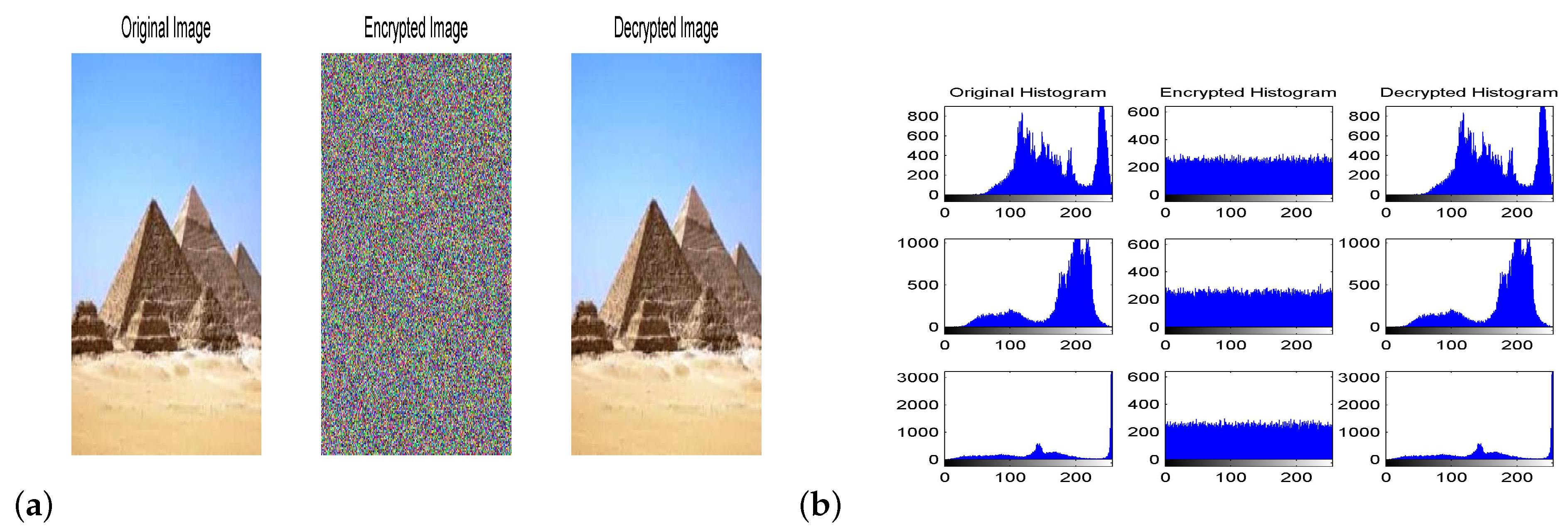
6.1. Numerical Simulations

Numerical simulations are performed at a = 2 , b = 3.35 , c = 9.15 , μ k = 0.1250075381 + 10 3 k and α = 0.985 . Figure 12a shows the plain King Tut image, ciphered King Tut image and deciphered King Tut image. The histograms for separate colors components in the pixels of these images are given in Figure 12b. In addition, Figure 13, Figure 14 and Figure 15 show the results correspond to images of Baboon, pepper and Egyptian pyramids, respectively. It is clear that the distribution of pixels’ values in encrypted images is almost flat and uniform for each color which renders the encrypted images invulnerable to different statistical attacks.
The uniformity of pixels distribution in ciphered images is quantified using the variance of histogram concept. More specifically, the small values of variances indicate high level uniformity. It can be defined for red, green and blue colors as follows:
v R = 1 256 2 i = 1 256 j = 1 256 ( h i R h j R ) 2 , v G = 1 256 2 i = 1 256 j = 1 256 ( h i G h j G ) 2 , v B = 1 256 2 i = 1 256 j = 1 256 ( h i B h j B ) 2 ,
where h i R , h i G and h i B are the number of pixels with the value of i for red, green and blue values of pixels, respectively. The results obtained for each image are summarized in Table 1. The results show the considerable reduction in variances of histograms for cipher images and thus confirm the uniformity of histogram values.

6.2. Keyspace Analysis

The proposed hybrid encryption technique has three initial conditions, four parameters of the model, i.e., a , b , c and α , three image-depending parameters μ i s . Suppose that the IEEE 754 floating-point format is used. Therefore, the secret keys of the proposed scheme will have space size equals 2 530 . This does not include the parameters of elliptic curve. Note that 2 100 space size is the minimum necessary size in order to break brute-force attacks [58,59]. Therefore, our encryption system has a big enough keyspace to make brute force attacks useless.

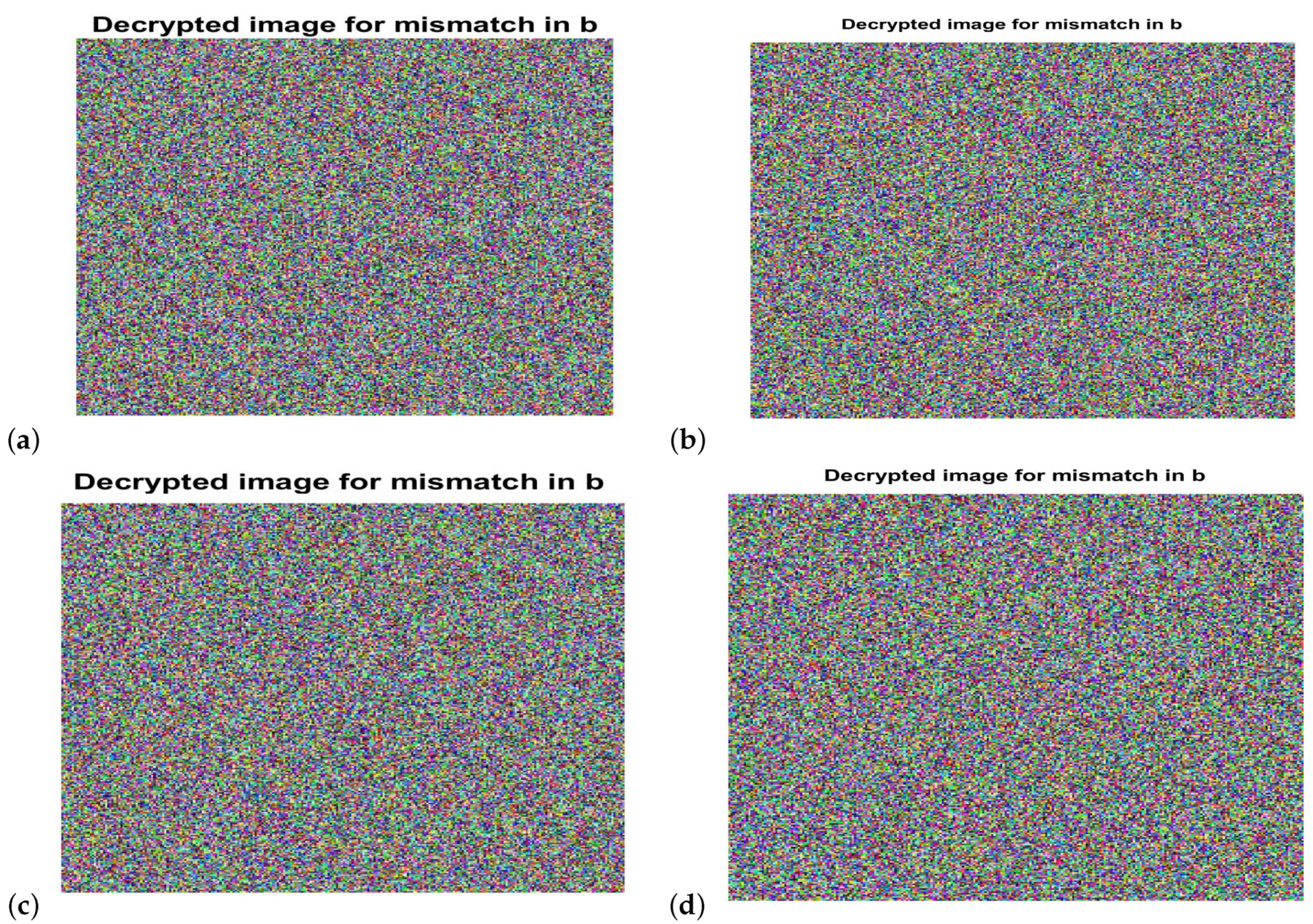
6.3. Analysis of Key Sensitivity

Another essential requirement for any reliable encryption scheme is to have high sensitivity to tiny perturbations in the values of secret keys. To investigate this point, the value of each secret key is perturbed by 10 14 at time and then the generated chaotic time series are used to decrypt the encrypted images. Then, the sensitivity to mismatch in parameters is investigated. Figure 16 shows an example when the value of b is perturbed by 10 14 . The deciphered images are shown in the figure. It is clear that when very small differences in b occur, we successfully decrypt any encrypted image. Numerical simulations illustrate that similar conclusions are inferred about the remaining secret keys in the system.
Finally, in order to measure the sensitivity to mismatches in parameters, Table 2 shows the original values of secret keys employed in encryption process, the mismatch of secret keys during decryption process, and the average difference percentage between the correct and incorrect decrypted images.

6.4. Analysis of Information Entropy

In order to investigate the degree of randomness and uncertainty of encrypted images, the information entropy is utilized. The large values of information entropy indicates high randomness of encrypted information. The information entropy has units in bits and it defined for an input information as follows [60]
H ( s ) = i = 0 2 N 1 p ( s i ) log ( s i ) ,
where s i denotes specific form i of input data, N is the number of possible different forms of input data and p ( s i ) refers to the probability of data symbol s i . Generally, the optimal value of H ( s ) of encrypted images is to be near to the value of 8. Table 3 illustrates the values of H ( s ) in the produced encrypted images. The computed values are almost equal to eight which shows the efficiency of the suggested technique.

6.5. Differential Attacks Analysis

For image encryption scheme to be efficient, it should be also very sensitive to teeny variations in plain images along with secret keys of encryption process. This shows that the very small perturbations that added to input data should make significant alternations in the resulting cipher data and hence the chaos based encryption scheme become more immune to different differential attacks [61,62,63].
For quantifying sensitivity to teeny changes in plain images, two measures can be successfully employed. The first of them is the Number of Pixels Change Rate (NPCR) that measures the percentage of unlike pixels between two encrypted images for one pixel difference in their associated plain images. The second measure is the Unified Average Changing Intensity (UACI), which represents the mean of intensity differences between two encrypted images for a single pixel value difference in the two input plain images.
Assume that C 1 and C 2 are two cipher images whose plain images are identical except for one pixel only. Let C 1 ( i , j ) and C 2 ( i , j ) refer to the specific color components of the pixel at position ( i , j ) in each of the two images. Thus, the NPCR is defined by [64,65]
N P C R = 1 m × n i = 1 m j = 1 n Δ ( i , j ) × 100 % , Δ ( i , j ) = 1 C 1 ( i , j ) C 2 ( i , j ) 0 C 1 ( i , j ) = C 2 ( i , j ) .
The second measure is given by
U A C I = 1 m × n i = 1 m j = 1 n C 1 ( i , j ) C 2 ( i , j ) 255 × 100 % .
Table 4 presents the values of NPCR and UACI for difference in one color component in random single pixel of the two original images.

6.6. Resistance against Other Attacks

The Kerckhoff’s principle [66] states that through evaluation of security strength of a given encryption system, it should be assumed that the attacker has knowledge about the design and detailed structure of encryption system. The exception is the unknown values of secret keys. Taking this principle into account, there are four possible types of attacks, known as, known plaintext, ciphertext only, chosen plaintext (CP) and chosen ciphertext (CC) attacks, which can be utilized against the proposed system. Most importantly, the opponent in chosen ciphertext attack (CCA) can get access to the decryption system while in chosen plaintext attack (CPA), he secretly can establish access to the encryption system itself. Now, if the suggested cryptography system is immune to the aforementioned CCA and CCP, then the resistance against the other two types are confirmed [67,68].
The presented encryption scheme involves setting up the values of time-dependent and plain image-dependent parameters, scrambling of pixels, bit XOR of pixel values perturbing chaotic signal and elliptic curve key exchange as follows. Firstly, some key features are read out from the plain image to modify the original values of secret keys of the system. This indicates that different plain images will induce different cipher images even for the cases where input images having very small differences. Moreover, feeding the encryption machine with the same plain image, but at distinct times, will produce separated encrypted images because secret keys are time dependent on the moments that images are supplied to the system. In addition, assume that the attackers try to defeat the elliptic curve key exchange step to unveil the values of secret keys via applying the well known Pollard’s Rho attack or Baby Step, Giant Step attack [69,70,71,72]. The attacker will find that it is practically infeasible to achieve his goal. The interpretation is that although this attacks can obviously reduce the computations complexity of discrete logarithmic problem, it still requires approximately P E C = 7.9 × 10 28 of operations so as to break the encryption system. More specifically, it approximately requires more than 10 13 years to complete the attacking process utilizing 16 GB RAM and Intel Core i7-8550U CPU. Subsequently, the present hybrid technique is reliable against the known-plaintext and chosen-plaintext attacks [67,68] in addition to EC attacks.

7. Discussion and Conclusions

Analytical and numerical frameworks are presented to analyze a proposed discrete fractional-order food chain model. The present model exhibits rich dynamics and a variety of nonlinear phenomena is exhibited by its state variables.
It is the first model to consider discrete fractional order three-dimensional food chain model while the other models in literature are exclusively continuous time or integer-order discrete time models. The fractional order which represents the memory influences is found to have a significant impact on the stability of nontrivial fixed points of food chain model and it should not be ignored. More specifically, when the value of fractional order decreases from one, the stability of fixed point may be changed. For example, the fixed point E 1 is stable at a = 2.9 and b = 1 when fractional order is very close to one and it loses its stability and becomes unstable when α = 0.8 . A second example is the fixed point E 2 which is stable at a = 3.05 and b = 2.4 , i.e., when the predator species has increased value of its benefit from predation on preys while simultaneously the fractional order value is very close to one. The fixed point E 2 losses its stability when α is decreased to 0.8. A third example is the coexistence fixed point E 3 which is stable at α > 0.88 , a = 3.05 , b = 3 and c = 4.35 while it losses its stability when α is decreased. Figure 1, Figure 2, Figure 3 and Figure 4 depict stability regions of fixed points in the space of parameters in more details. From biological point of view, the above discussion indicates that it possible to find two separate food chain systems which have identical values of parameters, i.e., same species for prey, predators and top-predators in the two systems, whilst the two systems undergo different stable equilibrium points. This can be therefore interpreted by referring to memory impacts or the different values of fractional order differences possessed by the two systems.
Employing multi-dimensional chaotic discrete fractional difference equations in encryption application is a very recent approach in cryptography systems. This approach overcomes numerical errors of continuous fractional order equations, has the advantages of extending the key space size by fractional order secret key and it is more appropriate for being implemented on digital platforms than the continuous time fractional systems. In addition, combining elliptic curve scheme for key exchange with the chaos source of three-dimensional fractional mapping in a novel hybrid encryption system, for first time, inherits the reliability and efficiency of both systems. From security point of view, the secret keys of the hybrid encryption system are made simultaneously time-varying and plain data-dependent that render the system capable to defeat the powerful CCA and CPA attacks along with other attacks, as discussed above. The realization on digital appliances can be conducted via using Arduino boards, such as ARDUINO NANO 33 BLE or ARDUINO MEGA 2560 REV3, Digital Signal Processors (DSPs), such as TMS320C6452 or ADSP-2136x, field-programmable gate array (FPGAs) or microcontrollers, such as nRF52840 or ATmega640. Future work may include adopting mixed functional response for the model to better reflect biological factors. In addition, the more advanced supersingular isogeny elliptic curves can be employed to further improve security strength of the proposed hybrid encryption scheme against risks of post quantum computers era.

Author Contributions

Conceptualization, S.A., A.A.-k., A.E. (Amr Elsonbaty) and A.E. (Abdelalim Elsadany); methodology, S.A., A.A.-k., A.E. (Amr Elsonbaty) and A.E. (Abdelalim Elsadany); software, S.A., A.A.-k., A.E. (Amr Elsonbaty) and A.E. (Abdelalim Elsadany); validation, S.A., A.A.-k., A.E. (Amr Elsonbaty) and A.E. (Abdelalim Elsadany); formal analysis, S.A., A.A.-k., A.E. (Amr Elsonbaty) and A.E. (Abdelalim Elsadany); investigation, S.A., A.A.-k., A.E. (Amr Elsonbaty) and A.E. (Abdelalim Elsadany); resources, S.A., A.A.-k., A.E. (Amr Elsonbaty) and A.E. (Abdelalim Elsadany); data curation, S.A., A.A.-k., A.E. (Amr Elsonbaty) and A.E. (Abdelalim Elsadany); writing—original draft preparation, S.A., A.A.-k., A.E. (Amr Elsonbaty) and A.E. (Abdelalim Elsadany); writing—review and editing, S.A., A.A.-k., A.E. (Amr Elsonbaty) and A.E. (Abdelalim Elsadany); visualization, S.A., A.A.-k., A.E. (Amr Elsonbaty) and A.E. (Abdelalim Elsadany); supervision, A.E. (Abdelalim Elsadany); project administration, S.A.; funding acquisition, S.A. All authors have read and agreed to the published version of the manuscript.

Funding

This work was supported by the Research Supporting Project Number (RSP2020/167), King Saud University, Riyadh, Saudi Arabia.

Acknowledgments

The authors would like to extend their sincere appreciation to King Saud University for funding this research (Project Number RSP2020/167).

Conflicts of Interest

The authors declare that they have no conflict of interests.

References

  1. Hilfer, R. Applications of Fractional Calculus in Physics; World Scientific: Singapore, 2000. [Google Scholar]
  2. Podlubny, I. Fractional Differential Equations: An Introduction to Fractional Derivatives; Elsevier: Amsterdam, The Netherlands, 1998. [Google Scholar]
  3. Baleanu, D.; Güvenç, Z.B.; Machado, J.T. (Eds.) New Trends in Nanotechnology and Fractional Calculus Applications; Springer: New York, NY, USA, 2010. [Google Scholar]
  4. Freeborn, T.J. A survey of fractional-order circuit models for biology and biomedicine. IEEE J. Emerg. Sel. Top. Circuits Syst. 2013, 3, 416–424. [Google Scholar] [CrossRef]
  5. Chen, W.C. Nonlinear dynamics and chaos in a fractional-order financial system. Chaos Solitons Fractals 2008, 36, 1305–1314. [Google Scholar] [CrossRef]
  6. Tarasova, V.V.; Tarasov, V.E. Elasticity for economic processes with memory: Fractional differential calculus approach. Fractional Differential Calc. 2016, 6, 219–232. [Google Scholar] [CrossRef]
  7. Magin, R.L. Fractional calculus models of complex dynamics in biological tissues. Comput. Math. Appl. 2010, 59, 1586–1593. [Google Scholar] [CrossRef] [Green Version]
  8. Hartley, T.T.; Lorenzo, C.F.; Qammer, H.K. Chaos in a fractional order Chua’s system. IEEE Trans. Circuits Syst. Fundam. Appl. 1995, 42, 485–490. [Google Scholar] [CrossRef]
  9. Yu, Y.; Li, H.X.; Wang, S.; Yu, J. Dynamic analysis of a fractional-order Lorenz chaotic system. Chaos Solitons Fractals 2009, 42, 1181–1189. [Google Scholar] [CrossRef]
  10. He, S.; Sun, K.; Wang, H. Complexity analysis and DSP implementation of the fractional-order Lorenz hyperchaotic system. Entropy 2015, 17, 8299–8311. [Google Scholar] [CrossRef] [Green Version]
  11. Sun, K.; Wang, X.; Sprott, J.C. Bifurcations and chaos in fractional-order simplified Lorenz system. Int. J. Bifurc. Chaos 2010, 20, 1209–1219. [Google Scholar] [CrossRef]
  12. Li, C.; Chen, G. Chaos in the fractional order Chen system and its control. Chaos Solitons Fractals 2004, 22, 549–554. [Google Scholar] [CrossRef]
  13. Wang, J.; Xiong, X.; Zhang, Y. Extending synchronization scheme to chaotic fractional-order Chen systems. Phys. Stat. Mech. Appl. 2006, 370, 279–285. [Google Scholar] [CrossRef]
  14. Liu, W.; Chen, Z. Dynamical behaviour of fractional-order atmosphere-soil-land plant carbon cycle system. AIMS Math. 2020, 5, 1532. [Google Scholar] [CrossRef]
  15. Li, Z.; Liu, L.; Dehghan, S.; Chen, Y.; Xue, D. A review and evaluation of numerical tools for fractional calculus and fractional order controls. Int. J. Control 2017, 90, 1165–1181. [Google Scholar] [CrossRef] [Green Version]
  16. Wang, Z.; Wang, Z.; Wu, B. September. Control and synchronization of fractional order complex valued chaotic Chen systems. J. Phys. Conf. Ser. 2018, 1074, 012101. [Google Scholar] [CrossRef]
  17. Song, C.; Fei, S.; Cao, J.; Huang, C. Robust synchronization of fractional-order uncertain chaotic systems based on output feedback sliding mode control. Mathematics 2019, 7, 599. [Google Scholar] [CrossRef] [Green Version]
  18. Li, G.; Zhang, X.; Yang, H. Numerical Analysis, Circuit Simulation, and Control Synchronization of Fractional-Order Unified Chaotic System. Mathematics 2019, 7, 1077. [Google Scholar] [CrossRef] [Green Version]
  19. Alizadeh, S.; Baleanu, D.; Rezapour, S. Analyzing transient response of the parallel RCL circuit by using the Caputo—Fabrizio fractional derivative. Adv. Differ. Equ. 2020, 2020, 55. [Google Scholar] [CrossRef]
  20. Wu, G.C.; Deng, Z.G.; Baleanu, D.; Zeng, D.Q. New variable-order fractional chaotic systems for fast image encryption. Chaos Interdiscip. J. Nonlinear Sci. 2019, 29, 083103. [Google Scholar] [CrossRef]
  21. Tsirimokou, G.; Psychalinos, C.; Elwakil, A. Design of CMOS Analog Integrated Fractional-Order Circuits: Applications in Medicine and Biology; Springer: Berlin/Heidelberg, Germany, 2017. [Google Scholar]
  22. Zhang, Y.; Liu, X.; Belic, M.R.; Zhong, W.; Zhang, Y.; Xiao, M. Propagation dynamics of a light beam in a fractional Schrodinger equation. Phys. Rev. Lett. 2015, 115, 180403. [Google Scholar] [CrossRef]
  23. Zhang, Y.; de Araujo, C.B.; Eyler, E.E. Higher-order correlation on polarization beats in Markovian stochastic fields. Phys. Rev. A 2001, 63, 043802. [Google Scholar] [CrossRef] [Green Version]
  24. Zhang, Y.; Gan, C.; Song, J.; Yu, X.; Ma, R.; Ge, H.; Li, C.; Lu, K. Coherent laser control in attosecond sum-frequency polarization beats using twin noisy driving fields. Phys. Rev. A 2005, 71, 023802. [Google Scholar] [CrossRef]
  25. Wu, G.C.; Baleanu, D. Discrete fractional logistic map and its chaos. Nonlinear Dyn. 2014, 75, 283–287. [Google Scholar] [CrossRef]
  26. Edelman, M.; Tarasov, V.E. Fractional standard map. Phys. Lett. A 2009, 374, 279–285. [Google Scholar] [CrossRef] [Green Version]
  27. Khennaoui, A.A.; Ouannas, A.; Bendoukha, S.; Wang, X.; Pham, V.T. On chaos in the fractional-order discrete-time unified system and its control synchronization. Entropy 2018, 20, 530. [Google Scholar] [CrossRef] [PubMed] [Green Version]
  28. Liu, Y. Chaotic synchronization between linearly coupled discrete fractional Hénon maps. Indian J. Phys. 2016, 90, 313–317. [Google Scholar] [CrossRef]
  29. Shukla, M.K.; Sharma, B.B. Investigation of chaos in fractional order generalized hyperchaotic Henon map. AEU Int. J. Electron. Commun. 2017, 78, 265–273. [Google Scholar] [CrossRef]
  30. Ji, Y.; Lai, L.; Zhong, S.; Zhang, L. Bifurcation and chaos of a new discrete fractional-order logistic map. Commun. Nonlinear Sci. Numer. Simul. 2018, 57, 352–358. [Google Scholar] [CrossRef]
  31. Fridrich, J. Image encryption based on chaotic maps. In Proceedings of the 1997 IEEE International Conference on Systems, Man, and Cybernetics. Computational Cybernetics and Simulation, Orlando, FL, USA, 12–15 October 1997; Volume 2, pp. 1105–1110. [Google Scholar]
  32. Lian, S.; Sun, J.; Wang, Z. Security analysis of a chaos-based image encryption algorithm. Phys. Stat. Mech. Appl. 2005, 351, 645–661. [Google Scholar] [CrossRef] [Green Version]
  33. Wang, X.; Liu, L. Cryptanalysis of a parallel sub-image encryption method with high-dimensional chaos. Nonlinear Dyn. 2013, 73, 795–800. [Google Scholar] [CrossRef]
  34. Tong, X.J. The novel bilateral–Diffusion image encryption algorithm with dynamical compound chaos. J. Syst. Softw. 2012, 85, 850–858. [Google Scholar] [CrossRef]
  35. Seyedzadeh, S.M.; Mirzakuchaki, S. A fast color image encryption algorithm based on coupled two-dimensional piecewise chaotic map. Signal Process. 2012, 92, 1202–1215. [Google Scholar] [CrossRef]
  36. Machado, J.A. Discrete-time fractional-order controllers. Fract. Calc. Appl. Anal. 2001, 4, 47–66. [Google Scholar]
  37. Wu, G.C.; Baleanu, D. Chaos synchronization of the discrete fractional logistic map. Signal Process. 2014, 102, 96–99. [Google Scholar] [CrossRef]
  38. Wu, G.C.; Baleanu, D.; Zeng, S.D. Discrete chaos in fractional sine and standard maps. Phys. Lett. A 2014, 378, 484–487. [Google Scholar] [CrossRef]
  39. Hu, T. Discrete chaos in fractional Hénon map. Appl. Math. 2014, 5, 2243–2248. [Google Scholar] [CrossRef] [Green Version]
  40. Abdeljawad, T. Different type kernel h- fractional differences and their fractional h- sums. Chaos Solitons Fractals 2018, 116, 146–156. [Google Scholar] [CrossRef]
  41. Khennaoui, A.A.; Ouannas, A.; Bendoukha, S.; Grassi, G.; Lozi, R.P.; Pham, V.T. On fractional—Order discrete—Time systems: Chaos, stabilization and synchronization. Chaos Solitons Fractals 2019, 119, 150–162. [Google Scholar] [CrossRef]
  42. Zhang, Y.; Xiao, D. Double optical image encryption using discrete Chirikov standard map and chaos-based fractional random transform. Opt. Lasers Eng. 2013, 51, 472–480. [Google Scholar] [CrossRef]
  43. Diab, H. An efficient chaotic image cryptosystem based on simultaneous permutation and diffusion operations. IEEE Access 2018, 6, 42227–42244. [Google Scholar] [CrossRef]
  44. Annaby, M.H.; Rushdi, M.A.; Nehary, E.A. Color image encryption using random transforms, phase retrieval, chaotic maps, and diffusion. Opt. Lasers Eng. 2018, 103, 9–23. [Google Scholar] [CrossRef]
  45. Qumsieh, R.; Farajallah, M.; Hamamreh, R. Joint block and stream cipher based on a modified skew tent map. Multimed. Tools Appl. 2019, 78, 33527–33547. [Google Scholar] [CrossRef]
  46. Wang, H.; Xiao, D.; Chen, X.; Huang, H. Cryptanalysis and enhancements of image encryption using combination of the 1D chaotic map. Signal Process. 2018, 144, 444–452. [Google Scholar] [CrossRef]
  47. Abdeljawad, T.; Banerjee, S.; Wu, G.C. Discrete tempered fractional calculus for new chaotic systems with short memory and image encryption. Optik 2019, 218, 163698. [Google Scholar] [CrossRef]
  48. Ridha, M.J. Image Scramble based on Discrete Cosine Transform and Henon Map. Iraqi J. Inf. Technol. 2019, 9, 96–107. [Google Scholar] [CrossRef]
  49. Deshpande, A.; Daftardar-Gejji, V. Chaos in discrete fractional difference equations. Pramana 2016, 87, 49. [Google Scholar] [CrossRef]
  50. Tarasova, V.V.; Tarasov, V.E. Exact discretization of an economic accelerator and multiplier with memory. Fractal Fract. 2017, 1, 6. [Google Scholar] [CrossRef]
  51. Girejko, E.; Pawl uszewicz, E.; Wyrwas, M. The Z-transform method for sequential fractional difference operators. In Theoretical Developments and Applications of Non-Integer Order Systems; Springer: Cham, Switzerland, 2016; pp. 57–67. [Google Scholar]
  52. Danca, M.F.; Feckan, M. Chaos suppression in a Gompertz-like discrete system of fractional order. arXiv 2019, arXiv:1908.11195. [Google Scholar] [CrossRef]
  53. Brandibur, O.; Kaslik, E.; Mozyrska, D.; Wyrwas, M. Stability of Systems of Fractional-Order Difference Equations and Applications to a Rulkov-Type Neuronal Model. In New Trends in Nonlinear Dynamics; Springer: Cham, Switzerland, 2020; pp. 305–314. [Google Scholar]
  54. Jouini, L.; Ouannas, A.; Khennaoui, A.A.; Wang, X.; Grassi, G.; Pham, V.T. The fractional form of a new three-dimensional generalized Hénon map. Adv. Differ. Equ. 2019, 2019, 122. [Google Scholar] [CrossRef]
  55. Xin, B.; Peng, W.; Kwon, Y. A fractional-order difference Cournot duopoly game with long memory. arXiv 2019, arXiv:1903.04305. [Google Scholar]
  56. Volterra, V. Variazioni e fluttuazioni del numero di individui in specie animali conviventi. Mem. Acad. Lincei. 1926, 2, 31–113. [Google Scholar]
  57. Lotka, A.J. Elements of Physical Biology; Williams and Wilkins: Baltimore, MD, USA, 1925. [Google Scholar]
  58. Kot, M. Elements of Mathematical Ecology; Cambridge University Press: Cambridge, MA, USA, 2001. [Google Scholar]
  59. Alsedà, L.; Vidiella, B.; Solé, R.; Lázaro, J.T.; Sardanyés, J. Dynamics in a time-discrete food-chain model with strong pressure on preys. Commun. Nonlinear Sci. Numer. Simul. 2020, 84, 105187. [Google Scholar] [CrossRef]
  60. ElGamal, T. A public key cryptosystem and a signature scheme based on discrete logarithms. IEEE Trans. Inf. Theory 1985, 31, 469–472. [Google Scholar] [CrossRef]
  61. Dăscălescu, A.C.; Boriga, R. A novel pseudo-random bit generator based on a new couple of chaotic systems. Ann. Ovidius Univ. Econ. Sci. Ser. 2011, 11, 553–558. [Google Scholar]
  62. Norouzi, B.; Mirzakuchaki, S. A fast color image encryption algorithm based on hyper-chaotic systems. Nonlinear Dyn. 2014, 78, 995–1015. [Google Scholar] [CrossRef]
  63. Hu, T.; Liu, Y.; Gong, L.H.; Ouyang, C.J. An image encryption scheme combining chaos with cycle operation for DNA sequences. Nonlinear Dyn. 2017, 87, 51–66. [Google Scholar] [CrossRef]
  64. Luo, Y.; Du, M.; Liu, J. A symmetrical image encryption scheme in wavelet and time domain. Commun. Nonlinear Sci. Numer. Simul. 2015, 20, 447–460. [Google Scholar] [CrossRef]
  65. Wu, Y.; Noonan, J.P.; Agaian, S. NPCR and UACI randomness tests for image encryption. Cyber J. Multidisciplinary J. Sci. Technol. 2011, 2, 31–38. [Google Scholar]
  66. Zhang, Y.-Q.; Wang, X.-Y. A symmetric image encryption algorithm based on mixed linear-nonlinear coupled map lattice. Inf. Sci. 2014, 273, 329–351. [Google Scholar] [CrossRef]
  67. Pareek, N.K.; Patidar, V.; Sud, K.K. Cryptography using multiple one- dimensional chaotic maps. Commun. Nonlinear Sci. Numer. Simul. 2005, 10, 715–723. [Google Scholar] [CrossRef]
  68. Ye, G.; Pan, C.; Huang, X.; Mei, Q. An efficient pixel-level chaotic image encryption algorithm. Nonlinear Dyn. 2018, 94, 745–756. [Google Scholar] [CrossRef]
  69. Wang, X.Y.; Teng, L.; Qin, X. Anovel colour image encryption algorithm based on chaos. Signal Process 2012, 92, 1101–1108. [Google Scholar] [CrossRef]
  70. Singh, K.M.; Singh, L.D.; Tuithung, T. Cryptanalysis of multimedia encryption using elliptic curve Cryptography. Optik 2018, 168, 370–375. [Google Scholar]
  71. Shanks, D. Class number, a theory of factorization, and genera. In Proceedings of the Symposia in Pure Mathematics; Number Theory Institute, State Univ. New York: Stony Brook, NY, USA, 1969; Volume XX, pp. 415–440. [Google Scholar]
  72. Pollard, J.M. Monte Carlo methods for index computation (mod p). Math. Comput. 1978, 32, 918–924. [Google Scholar]
Figure 1. Region of stability fixed point E 0 in (a, α ) plane.
Symmetry 13 00161 g001
Figure 2. Region of stability of fixed point E 1 in (a, α ) plane for (a) α = 0.8 and (b) α = 0.99 .
Symmetry 13 00161 g002
Figure 3. Stability region of fixed point E 2 in ( a , b ) plane for (a) α = 0.8 , (b) α = 0.9 and also in ( a , c ) plane for (c) α = 0.8 , (d) α = 0.9 .
Symmetry 13 00161 g003
Figure 4. Stability region of fixed point E 3 in ( a , b ) plane for α = 0.9 and (a) c = 3.9 and also in ( a , c ) plane for α = 0.9 and (b) b = 3 .
Symmetry 13 00161 g004
Figure 5. (ac) Time series of the state variables x , y and z of the stable fixed point E 0 at a = 0.5 , b = 1 , c = 1 and α = 0.9 .
Symmetry 13 00161 g005
Figure 6. (ac) Time series of the state variables x , y and z of the stable fixed point E 1 at a = 2 , b = 1 , c = 1 and α = 0.9 .
Symmetry 13 00161 g006
Figure 7. (ac) Time series of the state variables x , y and z of the stable fixed point E 2 at a = 3 , b = 2.5 , c = 0.9 and α = 0.8 .
Symmetry 13 00161 g007
Figure 8. (ac) Time series of the state variables x , y and z of the stable fixed point E 3 at a = 4 , b = 3 , c = 3.5 and α = 0.9 .
Symmetry 13 00161 g008
Figure 9. Bifurcation diagrams of parameters a and b vs. state variable x of (2) at (a) b = 4.6 , c = 3 and α = 0.95 , (b) a = 2.1 , c = 9.14 and α = 0.95 , respectively.
Symmetry 13 00161 g009
Figure 10. Bifurcation diagrams of (a) parameter α when a = 2 , b = 3.35 , c = 9.15 , (b) parameter b when a = 2 , c = 9.15 , α = 0.95 , (c) parameter b when a = 2 , c = 9.15 , α = 0.85 , (d) parameter α when a = 2.1 , b = 4.6 , c = 3 , (e) parameter a when b = 4.6 , c = 3 , α = 0.95 and (f) parameter b when a = 2.1 , c = 3 , α = 0.95 vs. state variable x of (2).
Symmetry 13 00161 g010
Figure 11. Examples of the two and three dimensional phase portraits of the models (1) and (2) obtained at (ac) a = 2 ; b = 4.6 ; c = 3 ; α = 1 , (df) a = 2 ; b = 3.1 ; c = 9.15 ; α = 1 , (gi) a = 2 ; b = 3.18 ; c = 9.15 ; α = 0.99 , (jl) a = 2 ; b = 3.25 ; c = 9.15 ; α = 0.99 and finally (mo) a = 2 ; b = 3.35 ; c = 9.15 ; α = 0.99 .
Symmetry 13 00161 g011
Figure 12. The plain, ciphered and deciphered King Tut images are shown in (a). The corresponding histograms of each color value are illustrated in (b) in the way that the first, second and third rows are representing, respectively, red, green and blue colors.
Symmetry 13 00161 g012
Figure 13. (a) The original, encrypted and decrypted image of a baboon face. (b) Histograms for those images given in (a).
Symmetry 13 00161 g013
Figure 14. (a) The original, encrypted and decrypted image of a pepper. (b) Histograms for those images given in (a).
Symmetry 13 00161 g014
Figure 15. (a) The original, encrypted and decrypted image of the Egyptian pyramids. (b) Histograms for those images given in (a).
Symmetry 13 00161 g015
Figure 16. Decrypted (a) King Tut image, (b) baboon image, (c) pepper image and (d) pyramids image for a mismatch in the value of b.
Symmetry 13 00161 g016
Table 1. The variances of plain and cipher images histograms.
Image v R v G v B
Original King Tut 6.45 × 10 4 1.11 × 10 5 1.63 × 10 4
Encrypted King Tut289293278
Original baboon 2.93 × 10 4 10 5 2.68 × 10 4
Encrypted baboon252248228
Original pepper 4.77 × 10 4 4 × 10 4 2.33 × 10 4
Encrypted pepper267309215
Original pyramids 3.06 × 10 4 1.57 × 10 5 2.61 × 10 5
Encrypted pyramids298209269
Table 2. Quantification of the sensitivity to mismatch in secret keys.
ImageKey ValueMismatch (%)Average Difference (%)
King Tut a = 2 10 10 99.56
King Tut b = 3.35 10 10 99.61
King Tut c = 9.15 10 10 99.54
Baboon a = 2 10 10 99.58
Baboon b = 3.35 10 10 99.55
Baboon c = 9.15 10 10 99.61
Pepper a = 2 10 10 99.63
Pepper b = 3.35 10 10 99.53
Pepper c = 9.15 10 10 99.59
Pyramids a = 2 10 10 99.62
Pyramids b = 3.35 10 10 99.64
Pyramids c = 9.15 10 10 99.66
Table 3. Information entropy in cipher images.
ImageInformation Entropy (R)(G)(B)
King Tut7.99757.99737.9977
Baboon7.99687.99667.9978
Pepper7.99677.99767.9967
Egyptian pyramids7.99727.99747.9975
Table 4. Number of Pixels Change Rate (NPCR) and Unified Average Changing Intensity (UACI) for the four encrypted images.
ImageNPCR (R, G, B) %UACI (R, G, B) %
King Tut99.6268, 99.6402, 99.636133.531, 33.531, 33.533
Baboon99.6332, 99.6329, 99.624133.537, 33.536, 33.536
Pepper99.6112, 99.6351, 99.629333.528, 33.506, 33.511
Egyptian pyramids99.6339, 99.6383, 99.615433.471, 33.483, 33.485
Publisher’s Note: MDPI stays neutral with regard to jurisdictional claims in published maps and institutional affiliations.

