Abstract
This paper starts with a review of three-dimensional chaotic dynamical systems equipped with special curves of balance points. We also propose the mathematical model of a new three-dimensional chaotic system equipped with a closed butterfly-like curve of balance points. By performing a bifurcation study of the new system, we analyze intrinsic properties such as chaoticity, multi-stability, and transient chaos. Finally, we carry out a realization of the new multi-stable chaotic model using Field-Programmable Gate Array (FPGA).
1. Introduction
Chaotic dynamical systems are applicable in a wide range of domains such as encryption [1,2,3], secure communication [4,5,6], robotics [7,8,9], lasers [10], chemical reactors [11], memristors [12,13,14], etc. Chen et al. [1] reported an optical image encryption algorithm in gyrator transform domain. Zhang [2] devised a new unified image encryption system with identical encryption and decryption algorithms. Hua et al. [3] developed a new color image encryption algorithm using a 2-D logistic tent modular map. Samimi et al. [4] designed a chaotic secure communication system with the help of a brain emotional learning-based intelligent controller. Abbasi et al. [5] proposed a chaotic evolutionary amino acid codons Model for image encryption. Alemami et al. [6] discussed chaos-based multiple encryption algorithms for speech recordings. Chaotic systems find use in secure communication devices and engineering applications featuring the implementations of analog or digital electronics [15].
Many types of chaotic dynamical systems have been studied in the literature such as jerk systems [16], butterfly attractors [17], multi-scroll systems [18,19,20], no-equilibrium chaotic systems [21,22,23], etc.
In the recent years, many papers have discussed the modeling of chaotic dynamical systems equipped with special curves having an infinite number of balance points [24].
Table 1 lists various dynamical systems exhibiting chaotic behavior with special curves of balance points such as hyperbola [25], circle [26], apple [27], axe [28], conch [29] and peanut [30].

Table 1.
Chaotic systems with special curves of balance points.
A main contribution of this work is the finding of a new chaotic dynamical system with a butterfly-like curve of balance points. We perform a bifurcation analysis of the new chaotic system and analyze its intrinsic properties such as multi-stability and transient chaos. Multi-stability refers to the coexistence of attractors of the new chaotic system, generated with different initial states of the system under fixed values of the parameters [31,32,33]. Transient chaos phenomenon occurs in a dynamical system when trajectories starting from randomly chosen initial conditions seem chaotic up to a certain time interval and then collapses into a periodic orbit or balance point with the evolution of time [34,35,36].
Furthermore, we carry out field-programmable gate array (FPGA) realization of the new chaotic system with a butterfly-like curve of balance points. Chaotic systems can be implemented in FPGA using numerical analysis and computer algorithms [37,38,39,40]. Realizations of chaotic systems using FPGA are useful for engineering applications such as generators of random numbers [41], secure devices [42], etc.
2. Mathematical Model of a Chaotic System with a Butterfly-Like Curve of Balance Points
The chaotic dynamical systems with special curves of balance points mentioned in Table 1 are particular cases of a general dynamical model stated as follows:
It is easy to observe that the balance points of the dynamical system (1) lie on the curve on the plane, which can be defined as follows:
In this research work, we define the mappings and as given below:
where are real, constant, parameters. We assume that are all positive.
Substituting (3) into (1), we obtain a new 3-D mathematical model as given below:
The balance points of the system (4) belong to the following curve on the plane.
The closed curve is symmetrical about both and coordinate cases in In the plane, looks like a butterfly as illustrated in Figure 1.
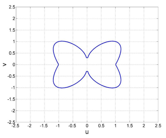
Figure 1.
The butterfly-like curve of balance points of the system (4) given by the following equations: (for all values of ).
The new dynamical model (4) exhibits a chaotic attractor if we take and the initial phase vector as the Lyapunov exponents spectrum can be calculated using Wolf’s algorithm [43] as and .
The presence of in the Lyapunov exponents spectrum () establishes the existence of a chaotic attractor of the system (4) [44]. Since we also conclude that the system (4) is a dissipative chaotic system [44].
The Kaplan-Yorke dimension [44] of a general n-D dissipative system with its Lyapunov exponents arranged in non-increasing order () is defined as follows:
where is the largest index such that .
Using the Formula (6), we determine the Kaplan-Yorke dimension of the system (4) as follows:
The large value of near three signifies the high complexity of the model (4).
The 2-D signal plots of the chaotic model (4) with butterfly-shaped curve of balance points for and the initial state are represented in Figure 2, Figure 3 and Figure 4.
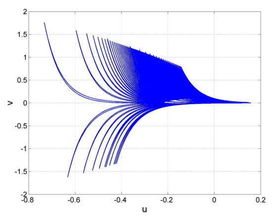
Figure 2.
The 2-D signal representation of the chaotic model (4) in the plane for the parameters and the initial state .
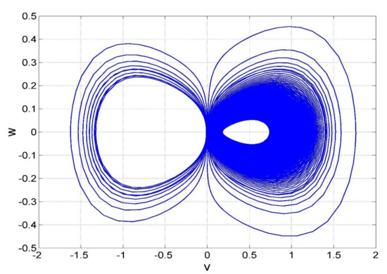
Figure 3.
The 2-D signal representation of the chaotic model (4) in the plane for the parameters and the initial state .
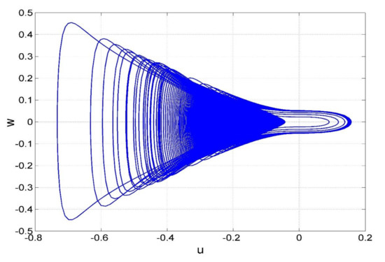
Figure 4.
The 2-D signal representation of the chaotic model (4) in the plane for the parameters and the initial state .
3. Dynamic Study of the Chaotic System with Butterfly-Molded Curve of Balance Points
In this section, we shall detail the bifurcation analysis, multi-stability, coexisting attractors and transient chaos of the new chaotic system (4) with butterfly-shaped equilibrium curve.
3.1. Bifurcation Study
In Section 2, it was shown that the system (4) is chaotic for For the bifurcation analysis, we take and . We consider the initial state as and . We vary in the range of The bifurcation range of the signal and the corresponding Lyapunov Exponents (LE) values is shown in Figure 5.
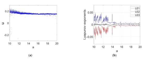
Figure 5.
Dynamic study of the chaotic system (4) with (a) The bifurcation diagram with respect to and (b) The Lyapunov exponents spectrum.
Figure 5 signifies robust chaos in the system (4) in the whole bifurcation region.
Next, we take and . We consider the initial state as and . We vary in the range of The bifurcation range of the state variable and the corresponding Lyapunov exponents is shown in Figure 6.
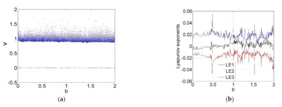
Figure 6.
Dynamic study of the chaotic system (4) with (a) The bifurcation diagram with respect to and (b) The Lyapunov exponents spectrum.
Figure 6 signifies robust chaos in the system (4) in the whole bifurcation region.
Next, we take and . We consider the initial state as and . We vary in the range of . The bifurcation range of the state variable and the corresponding Lyapunov exponents is shown in Figure 7.
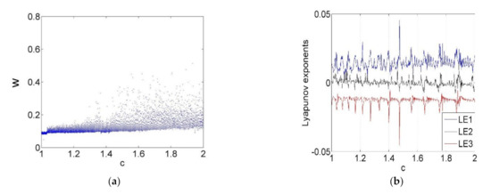
Figure 7.
Dynamic study of the chaotic system (4) with (a) The bifurcation diagram with respect to and (b) The Lyapunov exponents spectrum.
Figure 7 also signifies robust chaos in the system (4) in the whole bifurcation region.
Usually when analyzing the dynamics of a nonlinear system with parameter changes, it will encounter stable state, periodic chaos, and period-doubling bifurcation. However, for our system (4), only a chaotic state appears. The system (4) showing robust chaos is very advantageous in chaotic-based engineering applications, which can provide stable chaotic signals without external interference.
3.2. Multi-Stability
Multi-stability for a dynamical system undergoing chaotic behavior means the coexistence of two or more attractors with different initial states but fixed values of the system parameters [31,32,33].
We fix and vary in the region of . The initial states are selected as and . The coexisting bifurcation plot for the chaotic system (4) is represented in Figure 8.
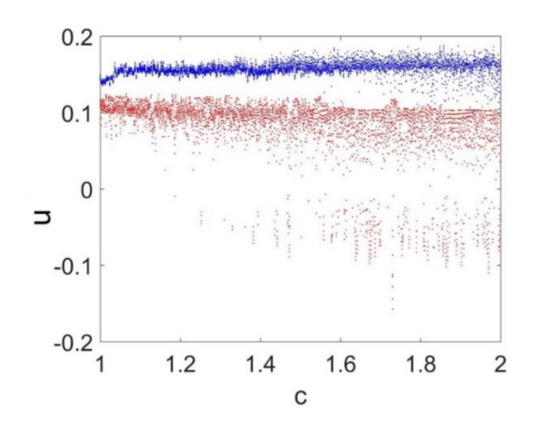
Figure 8.
The coexisting bifurcation diagram for the system (4) with respect to .
The blue color trajectory of the system (4) corresponds to the initial state while the red color trajectory of the system (4) corresponds to the initial state
When and the chaotic dynamical system (4) exhibits two types of coexisting chaotic attractors in Figure 9a,b, respectively.
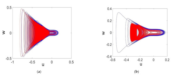
Figure 9.
Phase portraits of the coexisting chaotic attractors for the system (4) in the plane with varying the value of the parameter (a) the coexisting chaotic attractors for the system (4) for and (b) the coexisting chaotic attractors for .
3.3. Transient Chaos
Transient chaos means that a dynamical system is in a chaotic state at the beginning, and after time evolution, it eventually tends to a point or a periodic orbit [34,35,36]. When fixing and the system (4) exhibits transient chaos as represented in Figure 10. By calculating the Lyapunov exponents of transient chaos of the system (4) in interval [0, 225], we obtain the values of Lyapunov exponents as and
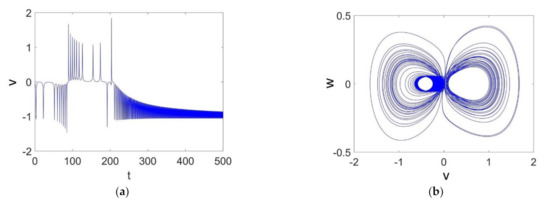
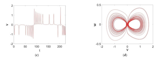
Figure 10.
Transient chaos pattern: (a) time series of in the interval ; (b) the phase portrait of the attractor in the plane; (c) time series of in the interval ; (d) the corresponding phase portrait of the attractor in the plane.
4. FPGA Realization of the Chaotic Dynamical System with a Butterfly-Like Curve of Balance Points
Here, we realize the new chaotic dynamical system (4) using FPGA. Chaotic systems are implemented in FPGA using finite-difference numerical schemes and computer algorithms [37,38,39,40].
The new dynamical system (4) with a closed butterfly-like curve of balance points can be represented in coordinate system as follows:
For FPGA implementation of the chaotic system (8), we need to discretize it first.
With the help of a forward Euler integration method [45], we obtain a discrete-time representation of the chaotic system as given below.
In the forward Euler scheme (9), and are the current and next counters respectively, while is the discretization step size.
Also, is the absolute value function, which is defined as follows:
The chaotic behavior of the system (8) can be obtained by selecting the coefficient parameters as and the initial phase as
A Python code for implementing the discretized chaotic system (9) is shown in Algorithm 1.
| Algorithm 1 Python code for the new discrete-time chaotic system (9) |
| Input: Initial states x0, y0, and z0. System parameters a, b, and c. Output: xn, yn, and zn j = 1 step = 500,000 x = x0 y = y0z = z0 while j < step do xn.insert(j, x + h ∗ z) yn.insert(j, y + h ∗ (z ∗ (−a ∗ y − b ∗ abs(y) − c ∗ x ∗ z)) zn.insert(j, z + h ∗ (pow(x,4) + pow(y,4) −abs(x) ∗ abs(y) − pow(x,2))) x = xn[j] y = yn[j] z = zn[j] j = j + 1 end |
Figure 11, Figure 12 and Figure 13 represent the simulated orbits for our chaotic oscillator system (7) using the Euler method (Algorithm 1) in the and planes, respectively with .
Figure 11.
The 2-D signal plot of the discrete-time chaotic system (9) using Forward Euler finite-difference scheme in the plane.
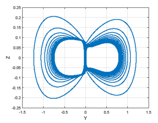
Figure 12.
The 2-D signal plot of the discrete-time chaotic system (9) using Forward Euler finite-difference scheme in the plane.
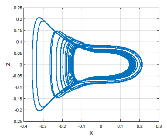
Figure 13.
The 2-D signal plot of the discrete-time chaotic system (9) using Forward Euler finite-difference scheme in the plane.
Figure 14 shows the top-level hardware design of the discrete-time chaotic system (8).
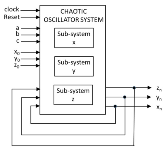
Figure 14.
Top-level hardware design of the discretized chaotic oscillator system (9).
The chaotic system (8) has three inputs for the initial phase signals and . In addition to the clock and reset signals, the chaotic system (9) has the system parameters and as the other inputs. As shown in Figure 14, the top-level block diagram contains three sub-systems, which are implemented according to Equations (9) and (10).
Each state variable in any of the chaotic sub-system has 32-bits. It is described using fixed-point representation which consists of 1-bit for the sign, 7-bits for the integer part, and 24-bits for the fractional part (see Figure 15).
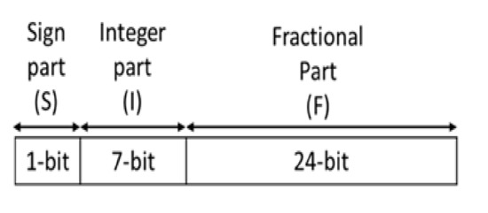
Figure 15.
32-bit fixed-point representation in a digital computer.
The Hardware Description Language (VHDL) code for the top level of the chaotic system (9) is devised as in [37].
The three sub-circuits are implemented using basic mathematical operations (Adder, Subtractor, Multiplier, Multiplexer, and Single Constant Multiplier). The basic blocks of these operations are shown in Figure 16. The VHDL codes for the adder/subtractor, and multiplier are taken as represented in [37].
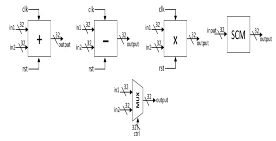
Figure 16.
Basic blocks for the three sub-circuits of the discrete-time chaotic system (9).
The Adder, Subtractor, and Multiplier blocks are sequential blocks with both clock (clk) and reset (rst) signals. The Single Constant Multiplier (SCM) performs a multiplication of the input by a constant with the use of only adders, subtractors, and shift operations. The Multiplexer (MUX) block chooses one of the inputs depending on the control signal (ctrl) and passes it to the output. In Figure 16, all inputs and outputs of the hardware blocks have a bus width of 32-bits.
In our hardware design, MUX is used to implement the absolute value function required for the state variables y and z. Hence, Equation (9) should be modified to use the multiplexer (MUX).
In the discrete equation of state variable the absolute value function is used, which is defined in Equation (11).
Equation (10) shows the state variable y after including MUX.
In the discrete equation of state variable two absolute functions are used, viz. and If both state variables have the same sign, then their multiplication is positive. Otherwise, it is negative. To check if the two state variables have the same sign, we need to XOR the sign bit of the state variable with the sign bit of the state variable i.e.,
Equation (12) shows the state variable z after including MUX.
To implement the sub-system the discrete equation of the signal in (9) is realized as represented in Figure 17. It uses SCM to multiply the signal by the constant and then adds the result to the signal to get the output
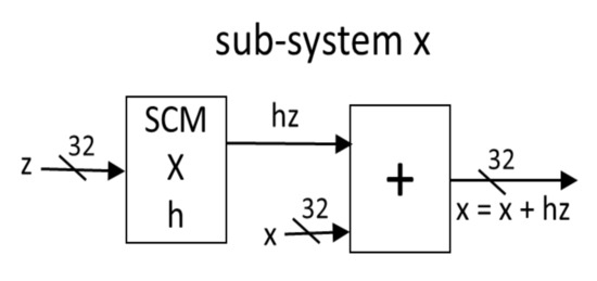
Figure 17.
Realization of the sub-system on FPGA.
To implement the sub-system the discrete equations of the signal in (11) are realized as represented in Figure 18. It uses four SCM modules, two multipliers, two adders, one subtractor, and one multiplexer. The SCM modules multiplies the input signals with a constant. The output signals are forwarded to the next modules. The multiplexer receives two signals produced by the adders and passes one of them according to the signal
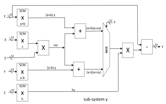
Figure 18.
Realization of the sub-system on FPGA.
To implement the sub-system the discrete equations of the signal in (12) are realized as represented in Figure 19. This sub-system is the most complex one. It includes seven multipliers, three adders, two subtractors, one SCM, and one multiplexer.
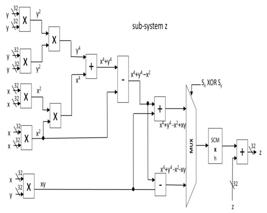
Figure 19.
Realization of the sub-system on FPGA.
The signal or is produced using three multipliers in two stages. The multiplexer receives two signals produced by an adder and a subtractor It passes one of them according to the result of The output of the multiplexer is multiplied by and added to the signal to produce the final output.
Our FPGA realization was carried out with the Zed-Board FPGA prototyping board from Xilinx. The system specifications of the board can be listed as Zynq-7000 all programmable SoC FPGA, 512 MB DDR3Memory, and some other peripherals. We synthesized the generated VHDL codes using Xilinx Vivado design suite and executed on the FPGA prototyping board.
Table 2 lists the FPGA resources use for each sub-system and for the complete chaotic oscillator system. As expected, the sub-system X uses less resources as it is less complex than the others. The sub-system Y uses more resources in addition to the Digital Signal Processors (DSPs) as it has more calculations. The sub-system Z is the most complex one. It requires 20 DSPs to perform seven multiplications and other operations.
Table 2.
FPGA resources use of sub-systems and complete chaotic oscillator system.
The complete implementation of discrete-time chaotic system (8) requires 390 Flip-Flops, 1295 Look-up Tables, 99 Input/outputs, and 28 DSPs. The use of the complete system does not exceed 0.37% of the total Flip-Flops, 2.43% of the total Look-up Tables, 12.73% of the DSPs available on the FPGA. The operation frequency of our chaotic oscillator system on the FPGA is 85.39 MHz.
5. Conclusions
Chaotic systems with special curves of balance points are studied with keen interest in the recent years. In this paper, we gave a concise review of three-dimensional chaotic systems equipped with open and closed curves of balance points. We presented a new three-dimensional chaotic system equipped with a closed butterfly-like curve of balance points in the (u,v)-plane. Using bifurcation analysis and Lyapunov exponent diagrams, we found many intrinsic properties such as chaoticity, multi-stability, and transient chaos. Finally, we carried out a realization of the new multi-stable chaotic model using FPGA.
Author Contributions
Modeling, A.S. and S.; methodology and writing, S.V.; MATLAB software and phase plots, Y.H., and G.G.; bifurcation analysis and multi-stability, S.Z.; FPGA design, T.B. Conceptualization, A.S. and S.; Formal analysis, Y.H. and M.M.; Methodology, S.V. and S.; Software, T.B., S.Z., Y.H. and G.G.; Supervision, M.M.; Validation, S.Z.; Writing—review & editing, S.V. All authors have read and agreed to the published version of the manuscript.
Funding
This research was funded Ministry of Research and Higher Education, Republik of Indonesia through Penelitian Kerja Sama Antar Perguruan Tinggi (Grant No. 01/SP2H/LIT-DRPM/LPPM/2020).
Conflicts of Interest
All the authors declare that there is no conflict of interest.
References
- Chen, H.; Liu, Z.; Tanougast, C.; Liu, F.; Blondel, W. A novel chaos based optical cryptosystem for multiple images using DNA-blend and gyrator transform. Opt. Lasers Eng. 2021, 138, 106448. [Google Scholar] [CrossRef]
- Zhang, Y. A new unified image encryption algorithm based on a lifting transformation and chaos. Inf. Sci. 2021, 547, 307–327. [Google Scholar] [CrossRef]
- Hua, Z.; Zhu, Z.; Yi, S.; Zhang, Z.; Huang, H. Cross-plane colour image encryption using a two-dimensional logistic tent modular map. Inf. Sci. 2021, 546, 1063–1083. [Google Scholar] [CrossRef]
- Samimi, M.; Majidi, M.H.; Khorashadizadeh, S. Secure communication based on chaos synchronization using brain emotional learning. AEU Int. J. Electron. Commun. 2020, 127, 153424. [Google Scholar] [CrossRef]
- Abbasi, A.A.; Mazinani, M.; Hosseini, R. Chaotic evolutionary-based image encryption using RNA codons and amino acid truth table. Opt. Laser Technol. 2020, 132, 106465. [Google Scholar] [CrossRef]
- Alemami, Y.; Mohamed, M.A.; Atiewi, S.; Mamat, M. Speech encryption by multiple chaotic maps with fast Fourier transform. Int. J. Electr. Comput. Eng. 2020, 10, 5658–5664. [Google Scholar] [CrossRef]
- Bazzi, S.; Sternad, D. Human control of complex objects: Towards more dexterous robots. Adv. Robot. Robt. 2020, 34, 1137–1155. [Google Scholar] [CrossRef]
- Fonseca, L.M.; Savi, M.A. Nonlinear dynamics of an autonomous robot with deformable origami wheels. Int. J. Non-Linear Mech. 2020, 125, 103533. [Google Scholar] [CrossRef]
- Yaghoubi, Z.; Zarabadipour, H. Hybrid neural-network control of mobile robot system via anti-control of chaos. Mech. Syst. Control 2020, 48, 239–248. [Google Scholar] [CrossRef]
- Liu, S.; Jiang, N.; Zhao, A.; Zhang, Y.; Qiu, K. Chaos synchronization and communication in global semiconductor laser network with coupling time delay signature concealment. Appl. Opt. 2020, 59, 6788–6795. [Google Scholar] [CrossRef]
- Schenkendorff, R.; Xie, X.; Krewer, U. An efficient polynomial chaos expansion strategy for active fault identification of chemical processes. Comput. Chem. Eng. 2019, 122, 228–237. [Google Scholar] [CrossRef]
- Xiu, C.; Zhou, R.; Liu, Y. New chaotic memristive cellular neural network and its application in secure communication system. Chaos Solitons Fract. 2020, 141, 110316. [Google Scholar] [CrossRef]
- Yildirim, M.; Kacar, F. Chaotic circuit with OTA based memristor on image cryptology. AEU Int. J. Electron. Commun. 2020, 127, 153424. [Google Scholar] [CrossRef]
- Caldarola, F.; Pantano, P.; Bilotta, E. Computation of supertrack functions for Chua’s oscillator and for Chua’s circuit with memristor. Commun. Nonlinear Sci. Numer. Simul. 2021, 94, 105568. [Google Scholar] [CrossRef]
- Tlelo-Cuautle, E.; Pano-Azucena, A.D.; Guillén-Fernández, O.; Silva-Juárez, A. Analog/Digital Implementation of Fractional Order Chaotic Circuits and Applications; Springer: Berlin/Heidelberg, Germany, 2020. [Google Scholar]
- Ding, P.F.; Feng, X.Y.; Wu, C.M. Novel two-directional grid multi-scroll chaotic attractors based on the jerk system. Chin. Phys. B 2020, 29, 108202. [Google Scholar] [CrossRef]
- Huang, Y. A five-dimensional grid multi-wing butterfly chaotic system and its circuit simulation. J. Phys. Conf. Ser. 2020, 1575, 012217. [Google Scholar] [CrossRef]
- Wang, F.; Zhu, B.; Wang, K.; Zhao, M.; Zhao, L.; Yu, J. Physical layer encryption in DMT based on digital multi-scroll chaotic system. IEEE Photonics Technol. Lett. 2020, 32, 1303–1306. [Google Scholar] [CrossRef]
- Mathale, D.; Doungmo Goufo, E.F.; Khumalo, M. Coexistence of multi-scroll chaotic attractors for fractional systems with exponential law and non-singular kernel. Chaos Solitons Fract. 2020, 139, 110021. [Google Scholar] [CrossRef]
- Liu, S.; Wei, Y.; Liu, J.; Chen, S.; Zhang, G. Multi-scroll chaotic system model and its cryptographic application. Int. J. Bifurc. Chaos 2020, 30, 2050186. [Google Scholar] [CrossRef]
- Nag Chowdhury, S.; Ghosh, D. Hidden attractors: A new chaotic system without equilibria. Eur. Phys. J. Spec. Top. 2020, 229, 1299–1308. [Google Scholar] [CrossRef]
- Singh, P.P.; Roy, B.K. A novel chaotic system without equilibria, with parachute and thumb shapes of Poincare map and its projective synchronisation. Eur. Phys. J. Spec. Top. 2020, 229, 1265–1278. [Google Scholar] [CrossRef]
- Lai, Q.; Wan, Z.; Kamdem Kuate, P.D. Modelling and circuit realisation of a new no-equilibrium chaotic system with hidden attractor and coexisting attractors. Electron. Lett. 2020, 56, 1044–1046. [Google Scholar] [CrossRef]
- Pham, V.T.; Vaidyanathan, S.; Volos, C.; Kapitaniak, T. Nonlinear Dynamical Systems with Self-Excited and Hidden Attractors; Springer: Berlin/Heidelberg, Germany, 2018. [Google Scholar]
- Vaidyanathan, S.; Sambas, A.; Lien, C.H.; Idowu, B.A. A new chaotic dynamical system with a hyperbolic curve of rest points, its complete synchronisation via integral sliding mode control and circuit design. Int. J. Model. Identif. Control 2019, 33, 198–207. [Google Scholar] [CrossRef]
- Sambas, A.; Sukono; Vaidyanathan, S.; Hidayat, Y.; Zhang, S.; Gundara, G.; Mohamed, M.A. Dynamic analysis and synchronization of a new chaotic system with a circle equilibrium and two perpendicular lines of equilibrium points. J. Adv. Res. Dyn. Control Syst. 2020, 12, 573–584. [Google Scholar]
- Sambas, A.; Sukono; Zhang, S.; Vaidyanathan, S.; Hidayat, Y.; Mujiarto. Electronic circuit design of a novel chaotic system with apple-shaped curve equilibrium and multiple coexisting attractors. J. Phys. Conf. Ser. 2020, 1477, 022015. [Google Scholar]
- Vaidyanathan, S.; Sambas, A.; Mamat, M. A new chaotic system with axe-shaped equilibrium, its circuit implementation and adaptive synchronization. Arch. Control Sci. 2018, 28, 443–462. [Google Scholar]
- Mamat, M.; Vaidyanathan, S.; Sambas, A.; Mohamed, M.A.; Sampath, S.; Sanjaya, W.S.M. A new 3-D chaotic system with conch-shaped equilibrium curve and its circuit implementation. Int. J. Eng. Tech. 2018, 7, 1410–1414. [Google Scholar] [CrossRef]
- Sambas, A.; Vaidyanathan, S.; Tlelo-Cuautle, E.; Abd-El-Atty, B.; El-Latif, A.A.A.; Guillen-Fernandez, O.; Sukono; Hidayat, Y.; Gundara, G. A 3-D multi-stable system with a peanut-shaped equilibrium curve: Circuit design, FPGA realization, and an application to image encryption. IEEE Access 2020, 8, 137116–137132. [Google Scholar] [CrossRef]
- Zhang, S.; Zeng, Y. A simple jerk-like system without equilibrium: Asymmetric coexisting hidden attractors, bursting oscillation and double full Feigenbaum remerging trees. Chaos Solitons Fract. 2019, 120, 25–40. [Google Scholar] [CrossRef]
- Zhang, S.; Zheng, J.; Wang, X.; Zeng, Z.; He, S. Initial offset boosting coexisting attractors in memristive multi double-scroll Hopfield neural network. Nonlinear Dyn. 2020. [Google Scholar] [CrossRef]
- Wang, N.; Zhang, G.; Kuznetsov, N.V.; Bao, H. Hidden attractors and multistability in a modified Chua’s circuit. Commun. Nonlinear Sci. Numer. Simul. 2021, 92, 105494. [Google Scholar] [CrossRef]
- Sabarathinam, S.; Thamilmaran, K. Transient chaos in a globally coupled system of nearly conservative Hamiltonian Duffing oscillators. Chaos Solitons Fract. 2015, 73, 129–140. [Google Scholar] [CrossRef]
- Zhang, S.; Zeng, Y.; Li, Z.; Wang, M.; Xiong, L. Generating one to four-wing hidden attractors in a novel 4D no-equilibrium chaotic system with extreme multistability. Chaos 2018, 28, 013113. [Google Scholar] [CrossRef] [PubMed]
- Zhang, S.; Wang, X.; Zeng, Z. A simple no-equilibrium chaotic system with only one signum function for generating multidirectional variable hidden attractors and its hardware implementation. Chaos 2020, 30, 053129. [Google Scholar] [CrossRef] [PubMed]
- Bonny, T. Chaotic or hyper-chaotic oscillator? Numerical solution, circuit design, MATLAB HDL-coder implementation, VHDL code, security analysis, and FPGA realization. Circuits Syst. Signal Process. 2020. [Google Scholar] [CrossRef]
- Bonny, T.; Nasir, Q. Clock glitch fault injection attack on an FPGA-based non-autonomous chaotic oscillator. Nonlinear Dyn. 2019, 96, 2087–2101. [Google Scholar] [CrossRef]
- Bonny, T.; Al Debsi, R.; Majzoub, S.; Elwakil, A.S. Hardware optimized FPGA implementations of high-speed true random bit generators based on switching-type chaotic oscillators. Circuits Syst. Signal Process. 2019, 38, 1342–1359. [Google Scholar] [CrossRef]
- Bonny, T.; Elwakil, A.S. FPGA realizations of high-speed switching-type chaotic oscillators using compact VHDL codes. Nonlinear Dyn. 2018, 93, 819–833. [Google Scholar] [CrossRef]
- Tuna, M. A novel secure chaos-based pseudo random number generator based on ANN-based chaotic and ring oscillator: Design and its FPGA implementation. Analog Integr. Circuits Signal Process. 2020, 105, 167–181. [Google Scholar] [CrossRef]
- Saber, M.; Hagras, E.A.A. Parallel multi-layer selector S-Box based on Lorenz chaotic system with FPGA implementation. Indones. J. Electr. Eng. Comput. Sci. 2020, 19, 784–792. [Google Scholar] [CrossRef]
- Wolf, A.; Swift, J.B.; Swinney, H.L.; Vastano, J.A. Determining Lyapunov Exponents from a time series. Phys. D Nonlinear Phenom. 1985, 16, 285–317. [Google Scholar] [CrossRef]
- Cencini, M.; Cecconi, F.; Vulpiani, A. Chaos from Simple Models to Complex Systems; World Scientific: Singapore, 2010. [Google Scholar]
- Chapra, S.; Canale, R. Numerical Methods for Engineers; McGraw-Hill: New York, NY, USA, 2014. [Google Scholar]


Publisher’s Note: MDPI stays neutral with regard to jurisdictional claims in published maps and institutional affiliations. |
© 2021 by the authors. Licensee MDPI, Basel, Switzerland. This article is an open access article distributed under the terms and conditions of the Creative Commons Attribution (CC BY) license (http://creativecommons.org/licenses/by/4.0/).