Quality Assessment of Groundwater Resources in the City of Al-Marj, Libya


Abstract
1. Introduction
2. Materials and Methodology
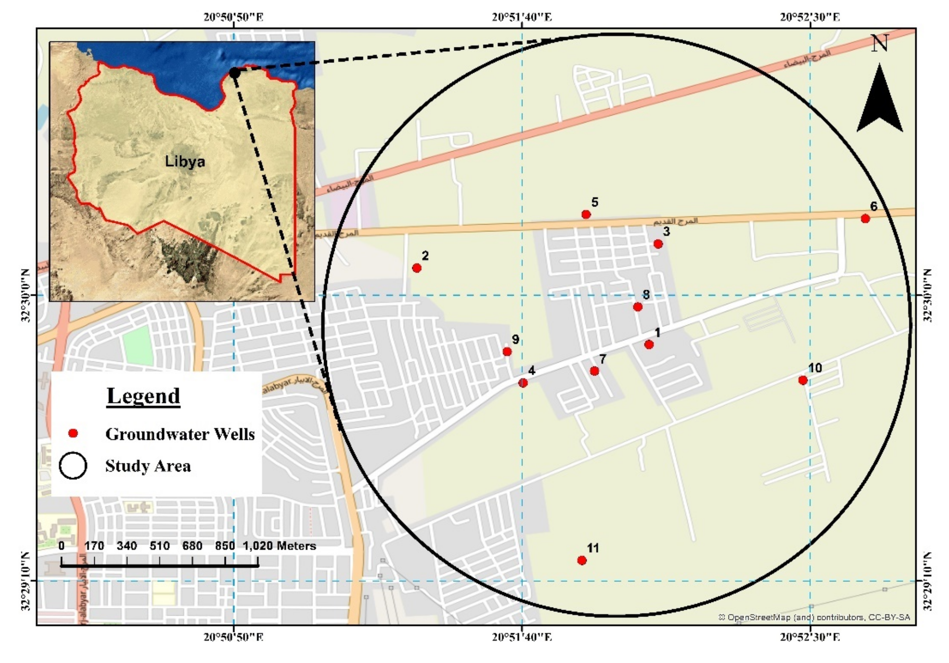
2.1. Description of the Study Area
2.2. Description of the Groundwater Wells
2.3. Sample Collection and Analysis
3. Results and Discussions
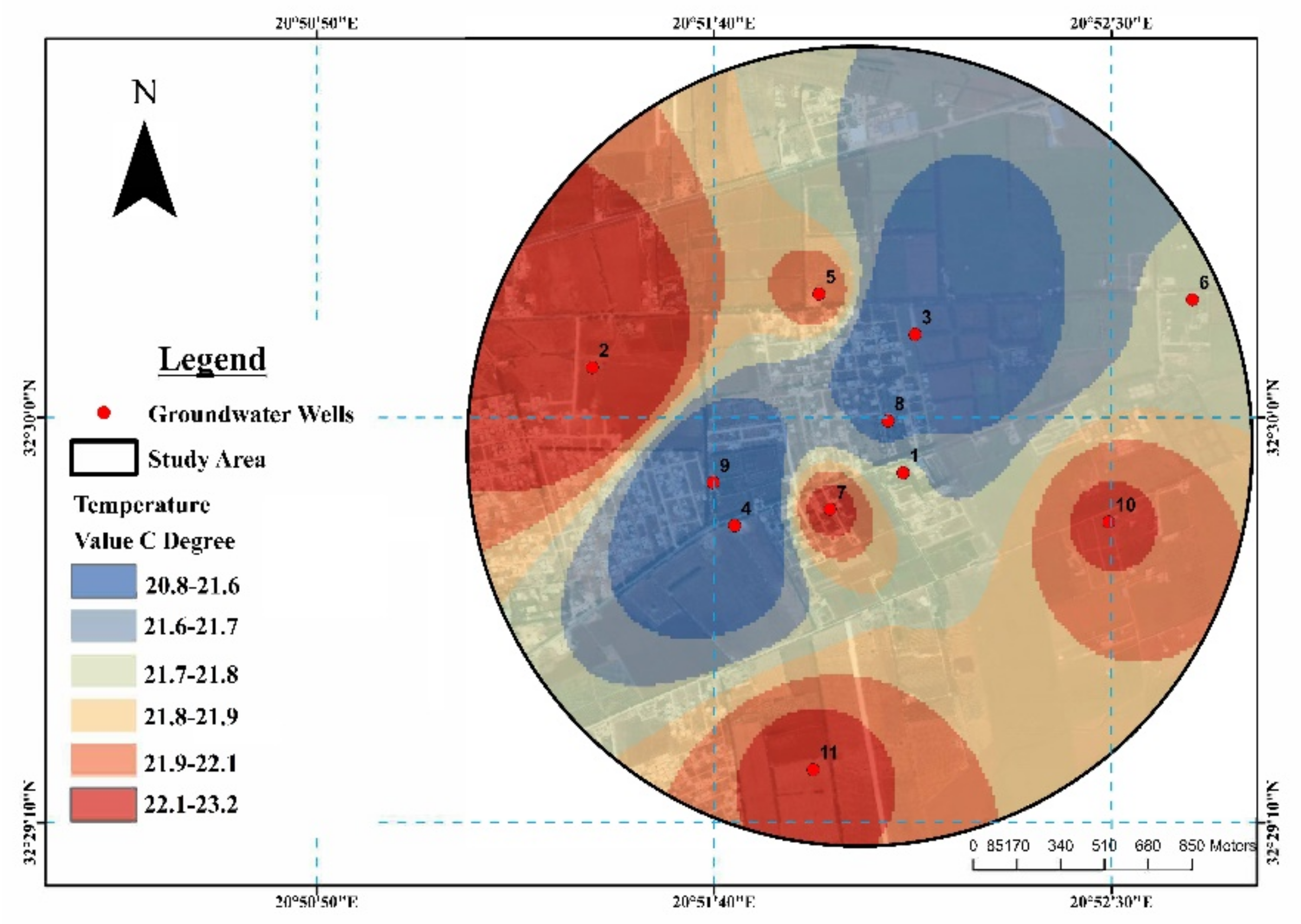
3.1. Temperature
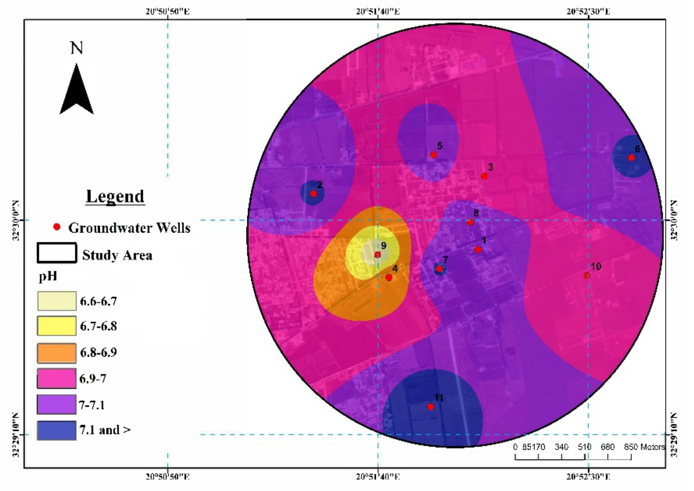
3.2. pH
3.3. Turbidity
3.4. Electrical Conductivity
3.5. Total Dissolved Solids
3.6. Chloride
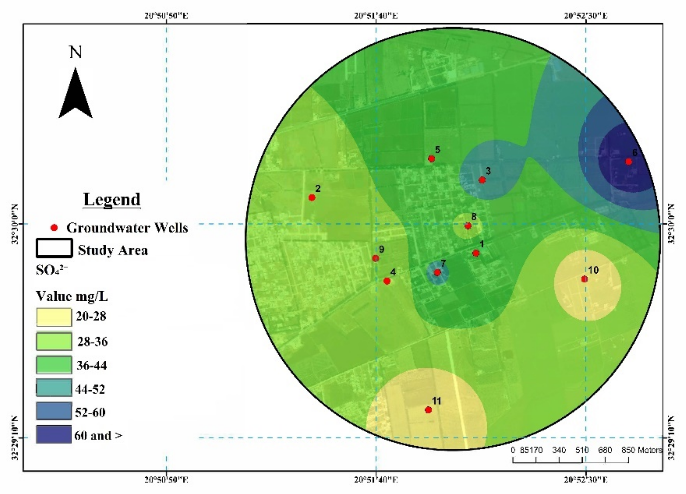
3.7. Sulphate
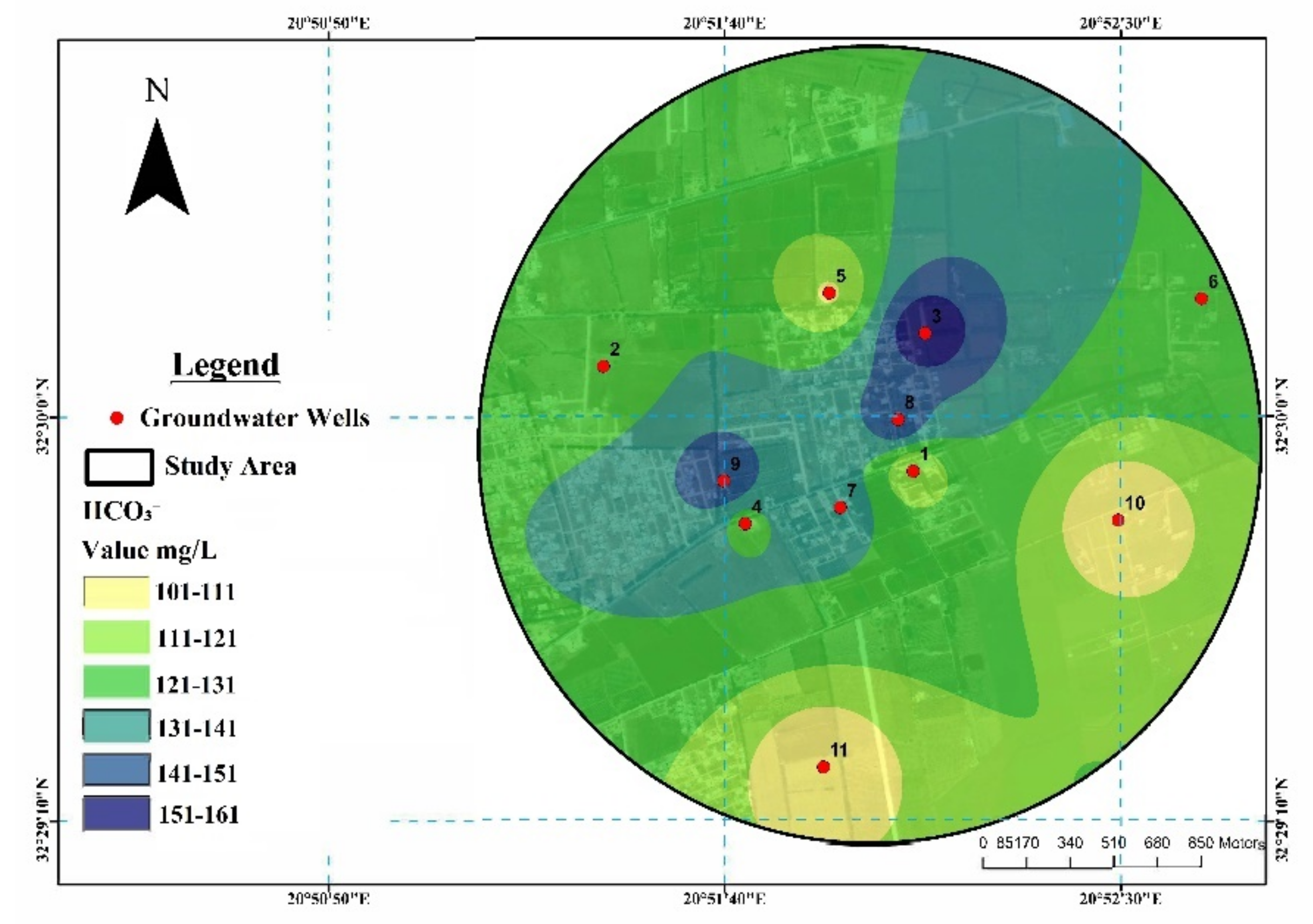
3.8. Bicarbonate
3.9. Total Hardness
3.10. Calcium
3.11. Potassium
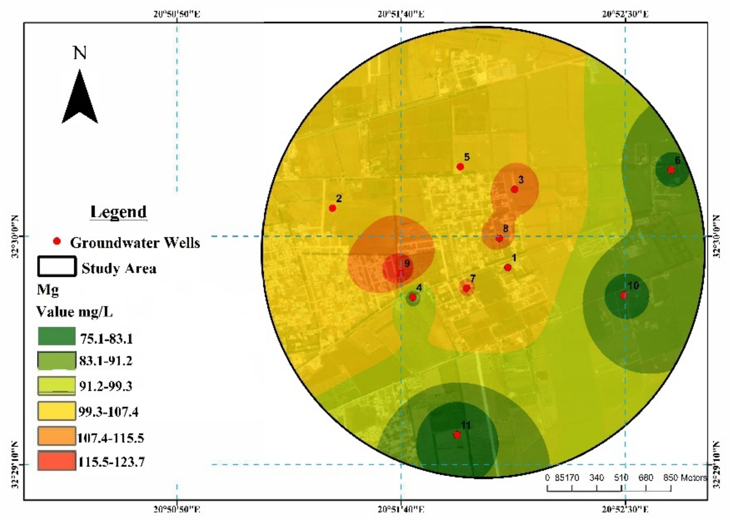
3.12. Magnesium
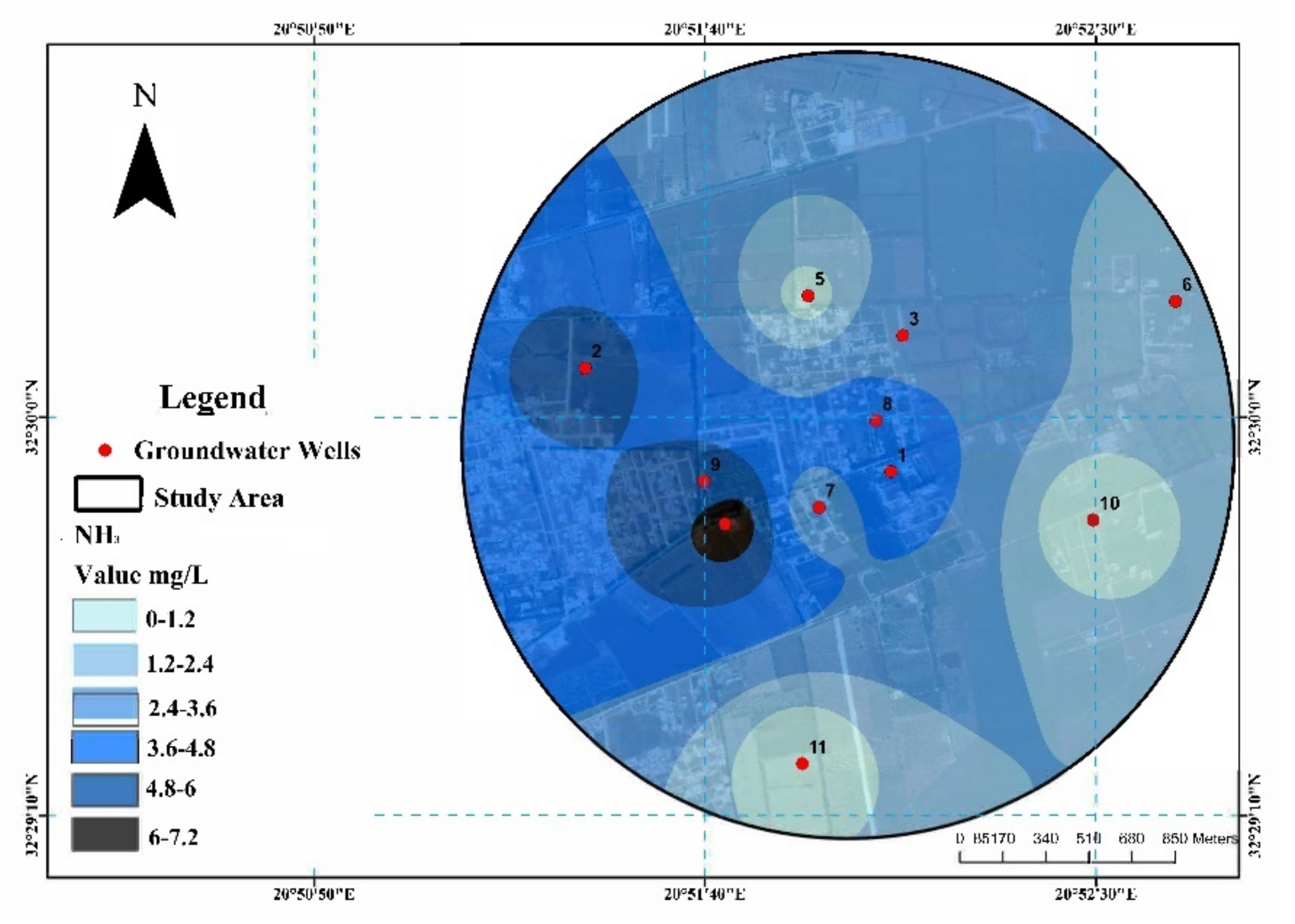
3.13. Ammonia
3.14. Ammoniacal Nitrogen
3.15. Nitrate
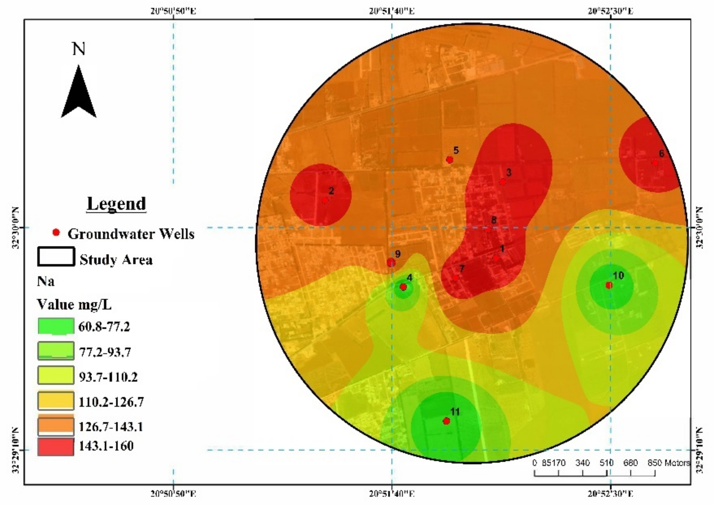
3.16. Sodium
3.17. Copper
3.18. Iron
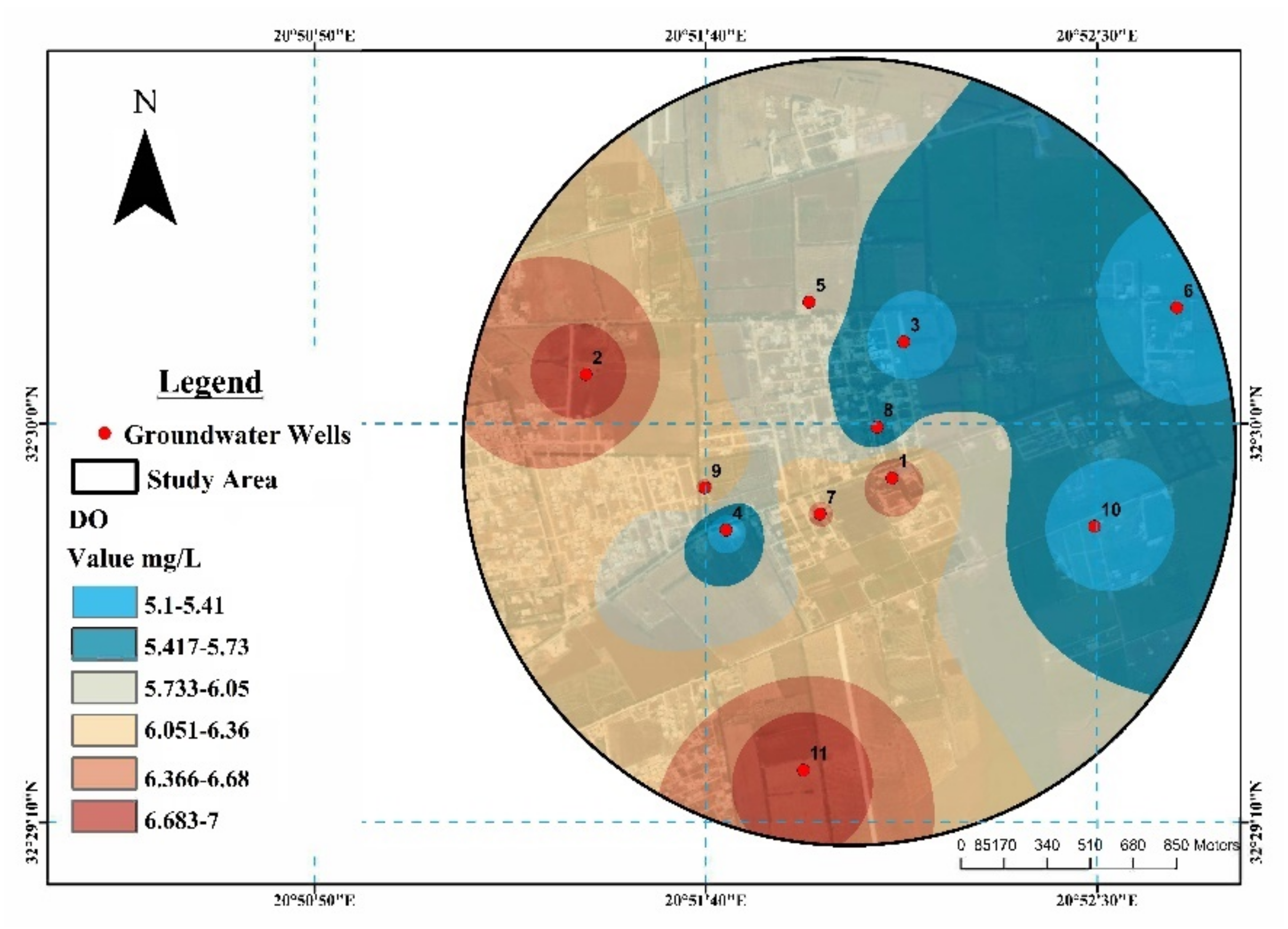
3.19. Dissolved Oxygen
3.20. Biological Oxygen Demand
3.21. Chemical Oxygen Demand
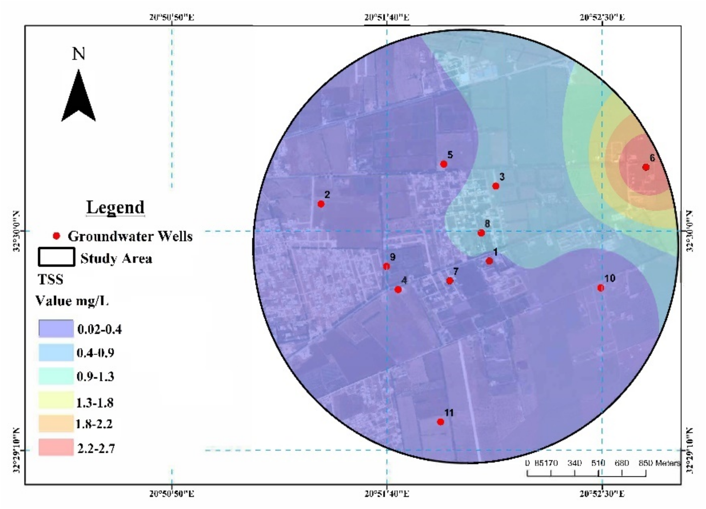
3.22. Total Suspended Solids
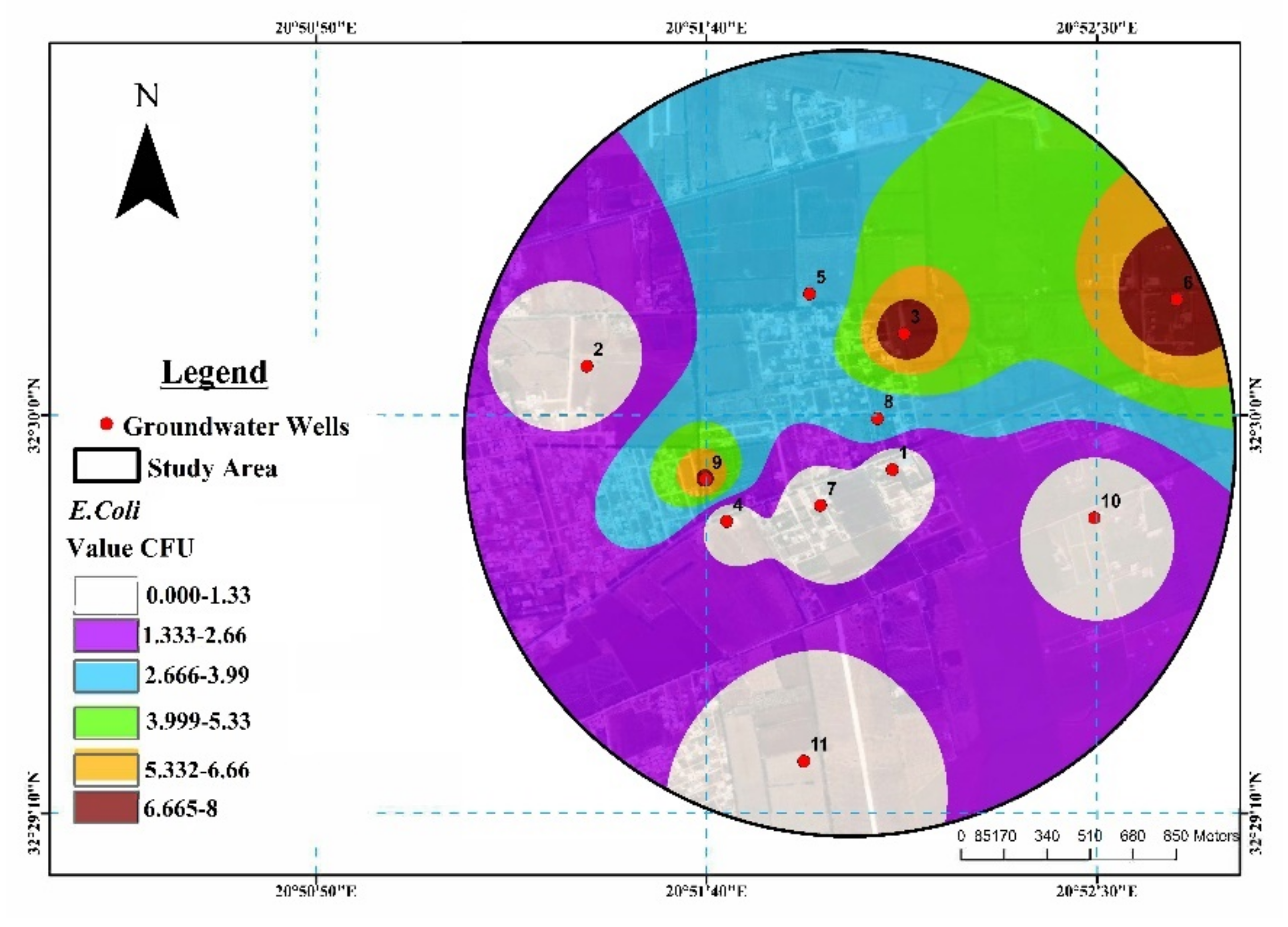
3.23. E. Coli
3.24. Total Coliforms
4. Conclusions
Author Contributions
Funding
Acknowledgments
Conflicts of Interest
References
- Hamzaoui-Azaza, F.; Ameur, M.; Bouhlila, R.; Gueddari, M. Geochemical characterization of groundwater in a Miocene Aquifer, Southeastern Tunisia. Environ. Eng. Geosci. 2012, 18, 159–174. [Google Scholar] [CrossRef]
- Nickson, R.T.; McArthur, J.M.; Shrestha, B.; Kyaw-Myint, T.O.; Lowry, D. Arsenic and other drinking water quality issues, Muzaffargarh District, Pakistan. Appl. Geochem. 2005, 20, 55–68. [Google Scholar] [CrossRef]
- Najafi Saleh, H.; Valipoor, S.; Zarei, A.; Yousefi, M.; Asghari, F.B.; Mohammadi, A.A.; Amiri, F.; Ghalehaskar, S.; Khaneghah, A.M. Assessment of groundwater quality around municipal solid waste landfill by using water quality index for groundwater resources and multivariate statistical technique: A case study of the landfill site, Qaem Shahr City, Iran. Environ. Geochem. Health 2020, 42, 1305–1319. [Google Scholar] [CrossRef] [PubMed]
- Loh, Y.S.A.; Akurugu, B.A.; Manu, E.; Aliou, A.S. Assessment of groundwater quality and the main controls on its hydrochemistry in some Voltaian and basement aquifers, northern Ghana. Groundw. Sustain. Dev. 2020, 10, 100296. [Google Scholar] [CrossRef]
- Wheida, E.; Verhoeven, R. An alternative solution of the water shortage problem in Libya. Water Resour. Manag. 2007, 21, 961–982. [Google Scholar] [CrossRef]
- Nair, G.A.; Bohjuari, J.A.; Al-Mariami, M.A.; Attia, F.A.; El-Toumi, F.F. Groundwater quality of north-east Libya. J. Environ. Biol. 2006, 27, 695–700. [Google Scholar]
- Jouda, J.H.R.; Hanafiah, M.M.; Yaakob, W.Z.W. Water resources management in Libya: Challenges and future prospects. Malaysian J. Sustain. Agric. 2017, 1, 2–5. [Google Scholar] [CrossRef]
- Tuinhof, A.; Foster, S.; van Steenbergen, F.; Talbi, A.; Wishart, M. Appropriate groundwater management policy for Sub-Saharan Africa. Appropr. Groundw. Manag. Policy Sub. Saharan Africa 2011. [Google Scholar] [CrossRef]
- Rashrash, S.M.; Ben Ghawar, B.M.; Hweesh, A.M. Evaluating groundwater pollution using hydrochemical data: Case study (Al Wahat Area East of Libya). J. Water Resour. Prot. 2015, 7, 369–377. [Google Scholar] [CrossRef]
- Abd El-Aziz, S.H. Evaluation of groundwater quality for drinking and irrigation purposes in the north-western area of Libya (Aligeelat). Environ. Earth Sci. 2017, 76. [Google Scholar] [CrossRef]
- Nnamani, E. Lack of Access to Potable Water Supply and Its Impact on the Nigerian Rural Communities. 2018. Available online: https://www.researchgate.net/publication (accessed on 23 December 2020).
- Jaouda, J.R.H.; Hanafiah, M.M.; Abdullah, S. Problems and current practices of solid waste management in the city of Al-marj, Libya. J. Clean WAS 2017, 1, 1–5. [Google Scholar] [CrossRef]
- El-Barasi, Y.M.; Saaed, M.W.B.; El-Amrouni, A.O.; Mohamad, N.F. Check list of flora and vegetation on south El-Marj zone: South El-Jabal El-Akhadar–Libya. Ann. Fac. Eng. Hunedora 2011, 9, 141. [Google Scholar]
- Bartram, J.; Ballance, R. Water Quality Monitoring–A Practical Guide to the Design and Implementation of Freshwater; Qual. Stud. Monit. Program; CRC Press: Boca Raton, FL, USA, 1996; pp. 1–348. ISBN 0-419-21730-4. Available online: https://apps.who.int/iris/handle/10665/41851 (accessed on 25 December 2020).
- Baird, R.B.; Eaton, A.D.; Rice, E.W.; Bridgewater, I. American Public Health Association (APHA). Standard Methods for the Examination of Water and Wastewater, 23th ed.; American Public Health Association/American Water Works Association/Water Environment Federation: Washington, DC, USA, 2017. [Google Scholar]
- Canadian Council of Ministers of the Environment (CCME). Introduction. Updated. In Canadian Environmental Quality Guidelines 1999; Canadian Council of Ministers of the Environment (CCME): Winnipeg, MB, Canada, 2001; Available online: https://www.ccme.ca/en/resources/canadian_environmental_quality_guidelines/ (accessed on 15 October 2020).
- Sayato, Y. WHO guidelines for drinking-water quality. Eisei Kagaku 1989, 35, 307–312. [Google Scholar] [CrossRef]
- HACH. Company. DR/890 Colorimeter Procedures Manual; HACH: Loveland, CO, USA, 2013; p. 616. [Google Scholar]
- Mostafa, H.; Al-wasify, R.S.; Sayed, A.M.; Bakry, M. Microbiological and Physicochemical Evaluation of Groundwater in Egypt. Int. J. Environ. Sustain. 2013, 2, 1–10. [Google Scholar] [CrossRef]
- Parmar, P.J. The studies on underground water quality of some villages of chalisgaon blocks along the north side of Girna Canal (Right) of Jalgaon. Oriental J. Chem. 2012, 28, 927–931. [Google Scholar] [CrossRef][Green Version]
- Nhua, H.E. Coseismic groundwater temperature response associated with the Wenchuan earthquake. Pageoph 2019. [Google Scholar] [CrossRef]
- Chacha, N.; Njau, K.N.; Lugomela, G.V.; Muzuka, A.N.N. Hydrogeochemical characteristics and spatial distribution of groundwater quality in Arusha well fields, Northern Tanzania. Appl. Water Sci. 2018, 8, 1–23. [Google Scholar] [CrossRef]
- Suk-ueng, K.; Chantima, K.; Prasertsin, T. Spatial distribution of soil quality using geoinformatics in agricultural areas in Nang Lae Sub-district, Mueang District, Chiang Rai Province. Intern. J. Agricult. Technol. 2019, 15, 779–790. [Google Scholar]
- World Health Organization (WHO). Guidelines for Drinking Water Quality [Electronic Resource]: Incorporating First Addendum. Volume 1, Recommenda-tions, 3rd ed.; WHO: Geneva, Switzerland, 2006; Available online: https://www.who.int/water_sanitation_health/dwq/gdwq0506.pdf (accessed on 5 October 2020).
- Brhane, G.K. Characterization of hydro chemistry and groundwater quality evaluation for drinking purpose in Adigrat area, Tigray, northern. TITLE Water Sci. 2018, 2017. [Google Scholar] [CrossRef]
- Nas, B.; Berktay, A. Groundwater quality mapping in urban groundwater using GIS. Environ. Monit. Assess. 2008, 160, 215–227. [Google Scholar] [CrossRef]
- Akinbile, C.O.; Yusoff, M.S. Environmental impact of leachate pollution on groundwater supplies in Akure, Nigeria. IJESD 2011. [Google Scholar] [CrossRef]
- Alfaifi, H.J.; Kahal, A.Y.; Abdelrahman, K.; Zaidi, F.K.; Albassam, A.; Lashin, A. Assessment of groundwater quality in Southern Saudi Arabia: Case study of Najran area. Arab. J. Geosci. 2020, 13, 1–15. [Google Scholar] [CrossRef]
- Dzwairo, B.; Hoko, Z.; Love, D.; Guzha, E. Assessment of the impacts of pit latrines on groundwater quality in rural areas: A case study from Marondera district, Zimbabwe. Phys. Chem. Earth 2006, 31, 779–788. [Google Scholar] [CrossRef]
- Qaseem, N.M.A.; Al-Barwary, M.R.A. Evaluation of physical and chemical quality of well water in Zakho District, Kurdistan region, Iraq Evaluation of physical and chemical quality of well water in Zakho District, Kurdistan region. Iraq. IOP Conf. 2018. [Google Scholar] [CrossRef]
- Mahmood, K.; Kamal, A.A.; Hama, A.R. Study and evaluation of stored drinking water characteristics using three types of roof water tanks in Kirkuk Governorate, Iraq. WJES 2018, 11–16. [Google Scholar] [CrossRef]
- Gopinath, G.; Laluraj, C.M. Assessment on seasonal variation of groundwater. Environ. Monit. Assess. 2006, 45–57. [Google Scholar] [CrossRef]
- El-salam, M.M.A.; Abu-zuid, G.I. Impact of landfill leachate on the groundwater quality: A case study in Egypt. J. Adv. Res. 2014. [Google Scholar] [CrossRef]
- Wei, Y.; Wu, S.; Chou, C.; Che, C.; Tsai, S.; H. Lien, H. Influence of nanoscale zero-valent iron on geochemical properties of groundwater and vinyl chloride degradation: A field case study. Water Res. 2009, 1–10. [Google Scholar] [CrossRef]
- Shah, M.; Sircar, A.; Shaikh, N.; Thakar, V.; Sharma, D.; Vaidya, D. Author’s accepted manuscript. Groundw. Sustain. Dev. 2018. [Google Scholar] [CrossRef]
- Geological, J.; Of, S. Factor and cluster analysis of water quality data of the Groundwater wells of Kushtia, Bangladesh: Implication for arsenic enrichment and mobilization. JGSI 2013, 81, 377–384. [Google Scholar]
- Lorite-Herrera, M.; Jiménez-Espinosa, R. Impact of agricultural activity and geologic controls on groundwater quality of the alluvial aquifer of the Gualquivir River (province of Jaen Spain): A case study. Environ. Geol. 2008, 1391–1402. [Google Scholar] [CrossRef]
- Biglari, H.; Chavoshani, A.; Javan, N.; Hossein Mahvi, A. Geochemical study of groundwater conditions with special emphasis on fluoride concentration, Iran. Desalin. Water Treat. 2016, 57, 22392–22399. [Google Scholar] [CrossRef]
- Boyd, C.E. Water Quality, An Introduction; Kluwer Academic Publishers: Boston, MA, USA, 2000; 330p. [Google Scholar]
- James, M. Spatial analysis of Groundwater sources in the duport road (shara and cow field) and soul clinic diamond creek communities, Paynesville City, Republic of Liberia. IJSRST 2017, 3, 1–12. [Google Scholar]
- Talat, R.A.; Al-Assaf, A.Y.; Al-Saffawi, A.Y. Valuation of water quality for drinking and domestic purposes using WQI: A case study for groundwater of Al-Gameaa and Al-Zeraee qaurters in Mosul city/Iraq. JPCS 2019. [Google Scholar] [CrossRef]
- Deshpande, S.M.; Aher, K.R.; Gaikwad, G.D. Assessment of groundwater quality and its suitability for drinking uses in warora tehsil, district chandrapur, India introduction. Int. J. Recent Trends Sci. Technol. 2012, 4, 120–124. [Google Scholar]
- Liaghat, S.M.S.K.E.A.M. Groundwater quality assessment using the Water Quality Index and GIS in Saveh-Nobaran aquifer, Iran. Science 2013. [Google Scholar] [CrossRef]
- Tikle, S.; Saboori, M.J.; Sankpal, R. Spatial distribution of ground water quality in some selected parts of pune city, Maharashtra, India using GIS. Curr. World Environ. 2012, 7, 281–286. [Google Scholar] [CrossRef][Green Version]
- Belkhiri, L.; Narany, T.S. Using multivariate statistical analysis, geostatistical techniques and structural equation modeling to identify spatial variability of Groundwater quality. Water Resour. Manag. 2015, 29, 2073–2089. [Google Scholar] [CrossRef]
- Kringel, R.; Rechenburg, A.; Kuitcha, D.; Fouépé, A.; Bellenberg, S.; Kengne, I.M.; Fomo, M.A. Mass balance of nitrogen and potassium in urban groundwater in Central Africa, Yaounde/Cameroon. Sci. Total Environ. 2016, 547, 382–395. [Google Scholar] [CrossRef]
- Shomar, B.; Fakher, S.A.; Yahya, A. Assessment of Groundwater quality in the Gaza strip, Palestine using GIS mapping. J. Water Resour. Prot. 2010, 2, 93–104. [Google Scholar] [CrossRef]
- Chenini, I.; Farhat, B.; Mammou, A.B. Identification of major sources controlling groundwater chemistry from a multilayered aquifer system. Chem. Speciat. Bioavailab. 2010, 22, 183–189. [Google Scholar] [CrossRef]
- Kouras, A.; Katsoyiannis, I.; Voutsa, D. Distribution of arsenic in groundwater in the area of Chalkidiki, Northern Greece. J. Hazard. Mater. 2007, 147, 890–899. [Google Scholar] [CrossRef]
- Kazi, T.G.; Arain, M.B.; Jamali, M.K.; Jalbani, N.; Afridi, H.I.; Sarfraz, R.A.; Baig, J.A.; Shahet, A.Q. Assessment of water quality of polluted lake using multivariate statistical techniques: A case study. Ecotoxicol. Environ. Saf. 2009, 72, 301–309. [Google Scholar] [CrossRef] [PubMed]
- Fu, Q.; Zheng, B.; Zhao, X.; Wang, L.; Liu, C. Ammonia pollution characteristics of centralized drinking water sources in China. J. Environ. Sci. 2012, 24, 1739–1743. [Google Scholar] [CrossRef]
- Harms-ringdahl, P. Identifying Possible Sources of Ammonium Ions and Arsenic in Groundwater in the Nam Du Area, Vietnam. Master’s Thesis, Hanoi Univ. of Mining and Geology Vietnam, Hanoi, Vietnam, 2007; p. 82. [Google Scholar]
- Jafari, M.T.; Khayamian, T. Direct determination of ammoniacal nitrogen in water samples using corona discharge ion mobility spectrometry. Talanta 2008, 76, 1189–1193. [Google Scholar] [CrossRef] [PubMed]
- Shakya, B.M.; Nakamura, T.; Kamei, T.; Das Shrestha, S.; Nishida, K. Seasonal groundwater quality status and nitrogen contamination in the shallow aquifer system of the Kathmandu Valley, Nepal. Water 2019, 11, 2184. [Google Scholar] [CrossRef]
- Wu, Z.; Ye, Q. Water pollution loads and shifting within China’s inter-province trade. J. Clean. Prod. 2020, 259, 120879. [Google Scholar] [CrossRef]
- Wakida, F.T.; Lerner, D.N. Non-agricultural sources of groundwater nitrate: A review and case study. Water Res. 2005, 39, 3–16. [Google Scholar] [CrossRef]
- Keeney, D.; Olson, R.A. Sources of nitrate to ground water. Crit. Rev. Environ. Control 1986, 16. [Google Scholar] [CrossRef]
- Wagh, V.M.; Panaskar, D.B.; Mukate, S.V.; Aamalawar, M.L.; Sahu, L.U. Nitrate associated health risks from groundwater of Kadava river Basin Nashik, Maharashtra, India. Hum. Ecol. Risk Assess. 2020, 26, 654–672. [Google Scholar] [CrossRef]
- El Hamidi, M.J.; Larabi, A.; Faouzi, M.; Souissi, M. Spatial distribution of regionalized variables on reservoirs and groundwater resources based on geostatistical analysis using GIS: Case of Rmel-Oulad Ogbane aquifers (Larache, NW Morocco). Arab. J. Geosci. 2018, 11. [Google Scholar] [CrossRef]
- Odoma, L.; Ocheri, M.I. Spatial Variability of Nitrate Levels in Groundwater of Lokoja Town, Kogi State, Nigeria. Curr. J. Appl. Sci. Technol. 2020, 39, 7–11. [Google Scholar] [CrossRef]
- Siemens, M.; Dynes, J.J.; Chang, W. Sodium adsorption by reusable zeolite adsorbents: Integrated adsorption cycles for salinised groundwater treatment. Environ. Technol. 2020, 1–41. [Google Scholar] [CrossRef] [PubMed]
- Rezaei, H.; Ryan, B.; Stoianov, I. Pipe failure analysis and impact of dynamic hydraulic conditions in water supply networks. Procedia Eng. 2015, 119, 253–262. [Google Scholar] [CrossRef]
- Adimalla, N.; Taloor, A.K. Hydrogeochemical investigation of groundwater quality in the hard rock terrain of South India using Geographic Information System (GIS) and groundwater quality index (GWQI) techniques. Groundw. Sustain. Dev. 2019, 100288. [Google Scholar] [CrossRef]
- Małecki, J.; Kadzikiewicz-Schoeneich, M.; Szostakiewicz-Hołownia, M. Concentration and mobility of copper and zinc in the hypergenic zone of a highly urbanized area. Environ. Earth Sci. 2016, 75, 1–13. [Google Scholar] [CrossRef]
- Santos, A.; Alonso, E.; Callejón, M.; Jiménez, J.C. Distribution of Zn, Cd, Pb and Cu metals in groundwater of the Guadiamar River Basin. Water. Air. Soil Pollut. 2002, 134, 275–286. [Google Scholar] [CrossRef]
- Yessuf, M.H. Geospatial study on characterization of Groundwater in Bheemunipatnam Municipality, Visakhapatnam District, Andhra Pradesh, India. IJERT 2018, 7, 175–184. [Google Scholar]
- Rajappa, B.; Manjappa, S.; Puttaiah, E. Monitoring of Heavy Metal Concentration in Groundwater of Hakinaka Taluk, India. Contemp. Eng. Sci. 2010, 3, 183–190. [Google Scholar]
- Kanoo, B.; Jawed, M. Assessing iron (II) and fluoride removals by indigenously fabricated household water filter of north Guwahati. Lect. Notes Civ. Eng. 2020, 57, 91–103. [Google Scholar] [CrossRef]
- Qiao, Y.; Zhu, X.; Jia, M.; Shao, X.; Niu, X.; Liu, J. Distributions of arsenic and other heavy metals, and health risk assessments for groundwater in the Guanzhong Plain region of China. Environ. Res. 2020, 181, 108957. [Google Scholar] [CrossRef] [PubMed]
- Zan, J.; Dong, Y.; Zhang, W.; Xu, W.; Li, J.; Gao, B.; Hu, F.; Wang, Q. Distribution characteristics of dissolved oxygen and stable isotope compositions of shallow groundwater in the vicinity of an inland nuclear power plant, HK, China. E3S Web Conf. 2019, 98, 4. [Google Scholar] [CrossRef]
- Yan, M.; Herrmann, B.; Kampe, R.; Lehmann, K.; Totsche, U.; Küsel, K. Environmental selection shapes the formation of near-surface groundwater microbiomes. Water Res. 2020, 170, 115341. [Google Scholar] [CrossRef] [PubMed]
- Owamah, H.I. A comprehensive assessment of groundwater quality for drinking purpose in a Nigerian rural Niger delta community. Groundw. Sustain. Dev. 2020, 10, 100286. [Google Scholar] [CrossRef]
- Abiriga, L.; Vestgarden, S.; Klempe, H. Groundwater contamination from a municipal landfill: Effect of age, landfill closure, and season on groundwater chemistry. Sci. Total Environ. 2020, 737, 140307. [Google Scholar] [CrossRef]
- Cox, B.A. A review of dissolved oxygen modelling techniques for lowland rivers. Sci. Total Environ. 2003, 314–316, 303–334. [Google Scholar] [CrossRef]
- Hanipha, A.; Hussain, Z. Study of Groundwater quality at Dindigul town, Tamilnadu, India. Int. Res. J. Environ. Sci. 2019, 2, 68–73. [Google Scholar]
- Koda, E.; Miszkowska, A.; Sieczka, A. Levels of organic pollution indicators in groundwater at the old landfill and waste management site. Appl. Sci. 2017, 7, 638. [Google Scholar] [CrossRef]
- Agbalagba, O.; Agbalagba, H.; Ononugbo, C.P.; Alao, A.A. Investigation into the physico-chemical properties and hydrochemical processes of groundwater from commercial boreholes In Yenagoa, Bayelsa State, Nigeria. Afr. J. Environ. Sci. Technol. 2011, 5, 473–481. [Google Scholar]
- González, S.O.; Almeida, C.A.; Calderón, M.; Mallea, M.A.; González, P. Assessment of the water self-purification capacity on a river affected by organic pollution: Application of chemometrics in spatial and temporal variations. Environ. Sci. Pollut. Res. 2014, 21, 10583–10593. [Google Scholar] [CrossRef]
- Negi, P.; Mor, S.; Ravindra, K. Impact of landfill leachate on the groundwater quality in three cities of North India and health risk assessment. Environ. Dev. Sustain. 2020, 22, 1455–1474. [Google Scholar] [CrossRef]
- Zhang, Z.; Yuan, Y.; Fang, Y.; Liang, L.; Ding, H.; Jin, L. Preparation of photocatalytic nano-ZnO/TiO2 film and application for determination of chemical oxygen demand. Talanta 2007, 73, 523–528. [Google Scholar] [CrossRef] [PubMed]
- Sajil Kumar, P.J.; Elango, L.; James, E.J. Assessment of hydrochemistry and groundwater quality in the coastal area of South Chennai, India. Arab. J. Geosci. 2014, 7, 2641–2653. [Google Scholar] [CrossRef]
- Ngang, B.U.; Agbazue, V.E. A seasonal assessment of Groundwater pollution due to biochemical oxygen demand, chemical oxygen demand and elevated temperatures in Enugu Northern Senatorial District, South East Nigeria. IOSR-JAC 2016, 9, 66–73. [Google Scholar] [CrossRef]
- Sojobi, A.O. Evaluation of groundwater quality in a rural community in North Central of Nigeria. Environ. Monit. Assess. 2016, 188, 1–17. [Google Scholar] [CrossRef]
- Hassan, A.; Nawaz, M. Microbiological and physicochemical assessments of groundwater quality at Punjab, Pakistan. Afr. J. Microbiol. Res. 2014, 8, 2672–2681. [Google Scholar] [CrossRef]
- Kumari, S.; Singh, A.K. Assessment and spatial distribution of groundwater quality in industrial areas of Ghaziabad, India. Environ. Monit. Assess 2013, 2014. [Google Scholar] [CrossRef]
- Bisiriyu, M.T.; Ganiyu, M.A.; Audu, L.I.; Abdullahi, A.S.; Animashaun, I.M. An Assessment of Groundwater Quality in Tudun Fulani, Niger State, Nigeria. SLUJST 2020, 1, 7–16. [Google Scholar]
- Figueras, M.J.; Borrego, J.J. New perspectives in monitoring drinking water microbial quality. Int. J. Environ. Res. Public Health 2010, 7, 4179–4202. [Google Scholar] [CrossRef]
- Yang, M.; Li, Y.; Wang, L.; Wang, L.; Niu, L. Hydrodynamic conditions influence bacterial growth and phenol biodegradation of strains with different morphology and motility. Water. Air. Soil Pollut. 2018, 229. [Google Scholar] [CrossRef]
- Daffi, R.E.; Alfa, M.I.; Ibrahim, E.S. Gis-based analysis of water quality parameters of Groundwater with proximity to onsite wastes pits in vom community of Jos South, Nigeria. J. Eng. Res. Rep. 2020, 10, 6–18. [Google Scholar] [CrossRef]
- Mkandawire, T. Quality of groundwater from shallow wells of selected villages in Blantyre District, Malawi. Phys. Chem. Earth 2008, 33, 807–811. [Google Scholar] [CrossRef]
- Invik, J.; Barkema, H.W.; Massolo, A.; Neumann, N.F.; Checkley, S. Total coliform and Escherichia coli contamination in rural well water: Analysis for passive surveillance. J. Water Health 2017, 15, 729–740. [Google Scholar] [CrossRef] [PubMed]
- Stokdyk, J.P.; Firnstahla, A.D.; Walshb, J.F.; Spencerc, S.K.; de Lambertb, J.R.; Anderson, A.C.; Rezania, L.-I.W.; Kieke, A.B., Jr.; Borchardt, M.A. Viral, bacterial, and protozoan pathogens and fecal markers in wells supplying groundwater to public water systems in Minnesota, MN, USA. Water Res. 2020, 178, 115814. [Google Scholar] [CrossRef]
- Kausch, M.E.; Fisher, S.C.; Fisher, I.J.; Phillips, P.J.; Mullan, G.D.O. Bacterial quality of groundwater downgradient of onsite wastewater disposal systems and the in fluence on eastern Long Island’s embayments. Mar. Pollut. Bull. 2019, 2018, 110598. [Google Scholar] [CrossRef]


| No. | Wells Name | Coordinates | Elevation (m) | Depth of wells (m) | Wells Age (Year) | |
|---|---|---|---|---|---|---|
| Latitude | Longitude | |||||
| 1 | Salah Amtaual | 32.497556 | 20.864528 | 284 | 280 | 1978 |
| 2 | Salam Edaab | 32.501167 | 20.853667 | 300 | 472 | 1979 |
| 3 | Al Marthi | 32.502306 | 20.864944 | 292 | 200 | 2001 |
| 4 | Saad Mokhtar | 32.495750 | 20.858639 | 297 | 228 | 1965 |
| 5 | Al Sahly | 32.503694 | 20.861583 | 296 | 200 | 1978 |
| 6 | Ali Ibrahim | 32.5035 | 20.874639 | 288 | 262 | 2010 |
| 7 | Agdora Al Abidi | 32.496306 | 20.861972 | 295 | 301 | 2002 |
| 8 | Mohamad Abd Raba | 32.499333 | 20.864 | 296 | 250 | 1999 |
| 9 | Sediq Al Rashed | 32.497222 | 20.857889 | 314 | 280 | 1978 |
| 10 | Idris Moftah | 32.436833 | 20.882028 | 356 | 365 | 1998 |
| 11 | Abo Shuisha | 32.428333 | 20.871694 | 363 | 300 | 2008 |
| Groundwater Wells | 1 | 2 | 3 | 4 | 5 | 6 | 7 | 8 | 9 | 10 | 11 |
|---|---|---|---|---|---|---|---|---|---|---|---|
| Mean | 21.8 | 23.2 | 20.8 | 21.2 | 22.1 | 21.8 | 22.3 | 21.6 | 21 | 22.2 | 22.3 |
| Std Dev | 2.9 | 1.2 | 2.2 | 2.6 | 1.2 | 1.9 | 2.1 | 1.5 | 2.5 | 2 | 2.4 |
| p-Value | 0.965 | ||||||||||
| WHO’s guideline | - | ||||||||||
| Groundwater Wells | 1 | 2 | 3 | 4 | 5 | 6 | 7 | 8 | 9 | 10 | 11 |
|---|---|---|---|---|---|---|---|---|---|---|---|
| Mean | 7.1 | 7.2 | 7 | 6.9 | 7.1 | 7.2 | 7.2 | 7.1 | 6.6 | 7 | 7.3 |
| Std Dev | 0.95 | 0.96 | 0.55 | 0.85 | 0.7 | 1.1 | 1.2 | 0.95 | 1.2 | 0.8 | 1 |
| p-Value | 0.99 | ||||||||||
| WHO’s guideline | 6.5–8.5 | ||||||||||
| Groundwater Wells | 1 | 2 | 3 | 4 | 5 | 6 | 7 | 8 | 9 | 10 | 11 |
|---|---|---|---|---|---|---|---|---|---|---|---|
| Mean | 0.2 | 0.3 | 1.2 | 0.4 | 0.5 | 0.6 | 0.7 | 0.8 | 0.6 | 0.2 | 0.3 |
| Std Dev | 0.08 | 0.1 | 0.8 | 0.2 | 0.2 | 0.4 | 0.2 | 0.4 | 0.09 | 0.2 | 0.2 |
| p-Value | 0.076 | ||||||||||
| WHO’s guideline | 5 |
| Groundwater Wells | 1 | 2 | 3 | 4 | 5 | 6 | 7 | 8 | 9 | 10 | 11 |
|---|---|---|---|---|---|---|---|---|---|---|---|
| Mean | 1479 | 1513 | 1711 | 1514 | 1564 | 1497 | 1648 | 1522 | 1530 | 905 | 826 |
| Std Dev | 16.5 | 4.6 | 10 | 16 | 3.6 | 15.5 | 8.5 | 9 | 95.6 | 13.1 | 11.5 |
| p-Value | 0.00 | ||||||||||
| WHO’s guidelines | 300 | ||||||||||
| Groundwater Wells | 1 | 2 | 3 | 4 | 5 | 6 | 7 | 8 | 9 | 10 | 11 |
|---|---|---|---|---|---|---|---|---|---|---|---|
| Mean | 739 | 757 | 854 | 756 | 782 | 748 | 824 | 761 | 765 | 452 | 412 |
| Std Dev | 12 | 12.3 | 4.5 | 13.5 | 3.6 | 11 | 8.2 | 8.5 | 6 | 18 | 4.6 |
| p-Value | 0.00 | ||||||||||
| WHO’s guidelines | 500 | ||||||||||
| Groundwater Wells | 1 | 2 | 3 | 4 | 5 | 6 | 7 | 8 | 9 | 10 | 11 |
|---|---|---|---|---|---|---|---|---|---|---|---|
| Mean | 288 | 283.4 | 353.1 | 285 | 281.3 | 284.4 | 319 | 282 | 282.6 | 147.6 | 134.3 |
| Std Dev | 11 | 3 | 6.5 | 14.7 | 7 | 9 | 6.2 | 4.6 | 7 | 10.1 | 5.7 |
| p-Value | 0.00 | ||||||||||
| WHO’s guideline | 250 | ||||||||||
| Groundwater Wells | 1 | 2 | 3 | 4 | 5 | 6 | 7 | 8 | 9 | 10 | 11 |
|---|---|---|---|---|---|---|---|---|---|---|---|
| Mean | 38 | 30 | 51 | 30 | 40.7 | 69 | 47 | 34 | 31.7 | 21.3 | 20 |
| Std Dev | 5.5 | 6 | 7.5 | 5.5 | 9.6 | 8.2 | 9.6 | 6.2 | 2.5 | 3.5 | 4 |
| p-Value | 0.00 | ||||||||||
| WHO’s guideline | 250 | ||||||||||
| Groundwater Wells | 1 | 2 | 3 | 4 | 5 | 6 | 7 | 8 | 9 | 10 | 11 |
|---|---|---|---|---|---|---|---|---|---|---|---|
| Mean | 111 | 125 | 161 | 128 | 110 | 131 | 135 | 151 | 151.3 | 101 | 101.7 |
| Std Dev | 3.6 | 8.7 | 8.5 | 7 | 7.5 | 6.5 | 6 | 8 | 3.8 | 4.6 | 3.5 |
| p-Value | 0.00 | ||||||||||
| WHO’s guideline | 300 | ||||||||||
| Groundwater Wells | 1 | 2 | 3 | 4 | 5 | 6 | 7 | 8 | 9 | 10 | 11 |
|---|---|---|---|---|---|---|---|---|---|---|---|
| Mean | 228 | 222 | 250.7 | 216 | 271 | 176 | 231 | 219 | 211.7 | 161 | 149 |
| Std Dev | 7 | 6.2 | 2.5 | 3.6 | 3.6 | 8 | 3 | 7.5 | 6.5 | 9.1 | 3.6 |
| p-Value | 0.00 | ||||||||||
| WHO’s guideline | 500 | ||||||||||
| Groundwater Wells | 1 | 2 | 3 | 4 | 5 | 6 | 7 | 8 | 9 | 10 | 11 |
|---|---|---|---|---|---|---|---|---|---|---|---|
| Mean | 124 | 116 | 140 | 127.7 | 167 | 94 | 122 | 110 | 123.7 | 81 | 74 |
| Std Dev | 3.6 | 8.1 | 4 | 6.5 | 5.3 | 4.6 | 3.6 | 6.2 | 3.5 | 2.1 | 6.6 |
| p-Value | 0.00 | ||||||||||
| WHO’s guideline | 75 | ||||||||||
| Groundwater Wells | 1 | 2 | 3 | 4 | 5 | 6 | 7 | 8 | 9 | 10 | 11 |
|---|---|---|---|---|---|---|---|---|---|---|---|
| Mean | 9.8 | 12 | 9.5 | 11.3 | 6.2 | 6.9 | 8.1 | 10.7 | 11.2 | 2.4 | 2.3 |
| Std Dev | 1.3 | 3 | 1.8 | 2.9 | 0.8 | 0.9 | 1.2 | 1.9 | 1.2 | 0.7 | 1.1 |
| p-Value | 0.00 | ||||||||||
| WHO’s guideline | 12 | ||||||||||
| Groundwater Wells | 1 | 2 | 3 | 4 | 5 | 6 | 7 | 8 | 9 | 10 | 11 |
|---|---|---|---|---|---|---|---|---|---|---|---|
| Mean | 104 | 106 | 110 | 88.3 | 104 | 82 | 108 | 109 | 123.7 | 80 | 75 |
| Std Dev | 3.6 | 4.4 | 2.6 | 3.1 | 2.6 | 3.6 | 6.6 | 13.1 | 3.5 | 4.6 | 10 |
| p-Value | 0.00 | ||||||||||
| WHO’s guideline | 150 | ||||||||||
| Groundwater Wells | 1 | 2 | 3 | 4 | 5 | 6 | 7 | 8 | 9 | 10 | 11 |
|---|---|---|---|---|---|---|---|---|---|---|---|
| Mean | 4.4 | 5.1 | 3 | 7 | 0.7 | 1.6 | 2.7 | 4.2 | 4.7 | 0.04 | 0.02 |
| Std Dev | 1.5 | 1.1 | 0.6 | 1 | 0.2 | 0.5 | 0.7 | 0.5 | 0.2 | 0.04 | 0.02 |
| p-Value | 0.00 | ||||||||||
| WHO’s guideline | 1.5 | ||||||||||
| Groundwater Wells | 1 | 2 | 3 | 4 | 5 | 6 | 7 | 8 | 9 | 10 | 11 |
|---|---|---|---|---|---|---|---|---|---|---|---|
| Mean | 3.7 | 4.3 | 2.5 | 5.8 | 0.6 | 1.3 | 2.2 | 3.5 | 3.7 | 0.03 | 0.01 |
| Std Dev | 1.5 | 1.2 | 0.7 | 0.6 | 0.1 | 0.5 | 0.8 | 0.5 | 0.2 | 0.03 | 0.02 |
| p-Value | 0.00 | ||||||||||
| WHO’s guideline | 0.1 | ||||||||||
| Groundwater Wells | 1 | 2 | 3 | 4 | 5 | 6 | 7 | 8 | 9 | 10 | 11 |
|---|---|---|---|---|---|---|---|---|---|---|---|
| Mean | 2.7 | 0.0 | 4.1 | 0.6 | 11 | 5 | 2.2 | 0.4 | 2.3 | 5.4 | 4.5 |
| Std Dev | 0.5 | 0.0 | 0.8 | 0.1 | 1.1 | 0.8 | 0.2 | 0.3 | 0.9 | 0.4 | 0.3 |
| p-Value | 0.00 | ||||||||||
| WHO’s guideline | 50 | ||||||||||
| Groundwater Wells | 1 | 2 | 3 | 4 | 5 | 6 | 7 | 8 | 9 | 10 | 11 |
|---|---|---|---|---|---|---|---|---|---|---|---|
| Mean | 153 | 149 | 160 | 63.8 | 136.3 | 150 | 155.3 | 144 | 145.7 | 65.7 | 60.8 |
| Std Dev | 14 | 8.5 | 8.1 | 4.3 | 9.5 | 8.7 | 6 | 8 | 5 | 12 | 6.9 |
| p-Value | 0.00 | ||||||||||
| WHO’s guideline | 200 | ||||||||||
| Groundwater Wells | 1 | 2 | 3 | 4 | 5 | 6 | 7 | 8 | 9 | 10 | 11 |
|---|---|---|---|---|---|---|---|---|---|---|---|
| Mean | 0.054 | 0.0035 | 0.0123 | 0.0021 | 0.0086 | 0.0083 | 0.0096 | 0.012 | 0.0096 | 0.001 | 0.0009 |
| Std Dev | 0.01 | 0.003 | 0.02 | 0.002 | 0.0017 | 0.014 | 0.0007 | 0.006 | 0.003 | 0.001 | 0.0007 |
| p-Value | 0.00 | ||||||||||
| WHO’s guideline | 2 | ||||||||||
| Groundwater Wells | 1 | 2 | 3 | 4 | 5 | 6 | 7 | 8 | 9 | 10 | 11 |
|---|---|---|---|---|---|---|---|---|---|---|---|
| Mean | 0.22 | 0.26 | 0.83 | 0.07 | 0.05 | 0.04 | 0.02 | 0.04 | 0.07 | 0.06 | 0.007 |
| Std Dev | 0.1 | 0.12 | 0.12 | 0.07 | 0.03 | 0.04 | 0.17 | 0.03 | 0.08 | 0.06 | 0.006 |
| p-Value | 0.00 | ||||||||||
| WHO’s guideline | 0.3 | ||||||||||
| Groundwater Wells | 1 | 2 | 3 | 4 | 5 | 6 | 7 | 8 | 9 | 10 | 11 |
|---|---|---|---|---|---|---|---|---|---|---|---|
| Mean | 6.7 | 6.9 | 5.1 | 5.2 | 5.9 | 5.2 | 6.4 | 5.4 | 6.4 | 5.2 | 7 |
| Std Dev | 1.2 | 1.3 | 0.56 | 0.46 | 0.82 | 0.53 | 0.81 | 1.25 | 1.41 | 0.4 | 0.9 |
| p-Value | 0.09 | ||||||||||
| WHO’s guideline | 4 | ||||||||||
| Groundwater Wells | 1 | 2 | 3 | 4 | 5 | 6 | 7 | 8 | 9 | 10 | 11 |
|---|---|---|---|---|---|---|---|---|---|---|---|
| Mean | 1.97 | 3.86 | 6.16 | 6.25 | 1.16 | 3.95 | 1.03 | 1.32 | 2.06 | 3.2 | 2.24 |
| Std Dev | 0 | 0.11 | 0.14 | 0.13 | 0.07 | 0.32 | 0.58 | 0.2 | 0.44 | 0.26 | 0.34 |
| p-Value | 0.00 | ||||||||||
| WHO’s guideline | 3 | ||||||||||
| Groundwater Wells | 1 | 2 | 3 | 4 | 5 | 6 | 7 | 8 | 9 | 10 | 11 |
|---|---|---|---|---|---|---|---|---|---|---|---|
| Mean | 4.41 | 8.25 | 9.26 | 9.34 | 2.13 | 10.1 | 2.25 | 3.7 | 3.07 | 5.62 | 3.61 |
| Std Dev | 0 | 0.2 | 0.7 | 0.3 | 0.1 | 0.1 | 0.1 | 0.1 | 0.4 | 0.3 | 0.2 |
| p-Value | 0.00 | ||||||||||
| WHO’s guideline | 10 | ||||||||||
| Groundwater Wells | 1 | 2 | 3 | 4 | 5 | 6 | 7 | 8 | 9 | 10 | 11 |
|---|---|---|---|---|---|---|---|---|---|---|---|
| Mean | 0.41 | 0.02 | 0.65 | 0.21 | 0.25 | 2.7 | 0.21 | 0.77 | 0.19 | 0.11 | 0.02 |
| Std Dev | 0 | 0.02 | 0.14 | 0.11 | 0.13 | 0.65 | 0.21 | 0.13 | 0.12 | 0.11 | 0.03 |
| p-Value | 0.00 | ||||||||||
| WHO’s guideline | NA | ||||||||||
| Groundwater Wells | 1 | 2 | 3 | 4 | 5 | 6 | 7 | 8 | 9 | 10 | 11 |
|---|---|---|---|---|---|---|---|---|---|---|---|
| Mean | 0.0 | 0.0 | 8.0 | 0.0 | 3.0 | 8.0 | 0.0 | 4.0 | 7.0 | 0.0 | 0.0 |
| Std Dev | 0 | 0 | 0 | 0 | 0 | 0 | 0 | 0 | 0 | 0 | 0 |
| p-Value | * | ||||||||||
| WHO’s guideline | 0 | ||||||||||
| Groundwater Wells | 1 | 2 | 3 | 4 | 5 | 6 | 7 | 8 | 9 | 10 | 11 |
|---|---|---|---|---|---|---|---|---|---|---|---|
| Mean | 0.0 | 0.0 | 240 | 0.0 | 39 | 460 | 0 | 39 | 210 | 7.0 | 0.0 |
| Std Dev | 0 | 0 | 0 | 0 | 0 | 0 | 0 | 0 | 0 | 0 | 0 |
| p-Value | * | ||||||||||
| WHO’s guideline | 0 | ||||||||||
Publisher’s Note: MDPI stays neutral with regard to jurisdictional claims in published maps and institutional affiliations. |
© 2021 by the authors. Licensee MDPI, Basel, Switzerland. This article is an open access article distributed under the terms and conditions of the Creative Commons Attribution (CC BY) license (http://creativecommons.org/licenses/by/4.0/).
Share and Cite
Hamad, J.R.J.; Yaacob, W.Z.; Omran, A. Quality Assessment of Groundwater Resources in the City of Al-Marj, Libya. Processes 2021, 9, 154. https://doi.org/10.3390/pr9010154
Hamad JRJ, Yaacob WZ, Omran A. Quality Assessment of Groundwater Resources in the City of Al-Marj, Libya. Processes. 2021; 9(1):154. https://doi.org/10.3390/pr9010154
Chicago/Turabian StyleHamad, Jauda R. Jauda, Wan Zuhairi Yaacob, and Abdelnaser Omran. 2021. "Quality Assessment of Groundwater Resources in the City of Al-Marj, Libya" Processes 9, no. 1: 154. https://doi.org/10.3390/pr9010154
APA StyleHamad, J. R. J., Yaacob, W. Z., & Omran, A. (2021). Quality Assessment of Groundwater Resources in the City of Al-Marj, Libya. Processes, 9(1), 154. https://doi.org/10.3390/pr9010154