Article

Method of Real-Time Wellbore Surface Reconstruction Based on Spiral Contour

1
School of Petroleum Engineering, China University of Petroleum, Qingdao 266580, China
2
Sinopec Shengli Drilling Technology Research Institute, Dongying 257000, China
*
Author to whom correspondence should be addressed.
Energies 2021, 14(2), 291; https://doi.org/10.3390/en14020291
Submission received: 5 December 2020 / Revised: 27 December 2020 / Accepted: 4 January 2021 / Published: 7 January 2021
(This article belongs to the Section H: Geo-Energy)

Abstract

:
A wellbore surface is an irregular surface structure. The distribution of points on the wellbore surface measured based on the drilling diameter is not uniform. Thus, the conventional modeling method based on a point cloud cannot satisfy the needs of real-time measurement updating and wellbore display. This study proposes a spiral profile method for drilling shaft surface reconstruction. Scattered data along the drilling diameter are measured, and an inverse distance weighting cylindrical space surface algorithm with iterative interpolation is used to obtain the spiral angle and pitch of a relatively homogeneous helical contour line along the surface of the shaft. Using sets of four adjacent points in the spiral, quadrilaterals are formed, and then all obtained quadrilaterals are used to form the wellbore inner surface structure. This method can further construct the outer surface spiral contour line to advance the quadrilateral surface to the spatial hexahedron structure. The caliper and gamma measurement data obtained from the calibrated wellbore were used to verify the real-time surface reconstruction and fusion while drilling. The homogenized reconstructed surface profile is more than 99.5% similar to the actual measurement. Proved by experiment and application, this method has very high real-time performance, and the three-dimensional stereo imaging wellbore with additional gamma attributes has good visual effects.

1. Introduction

When performing imaging measurement while drilling (IMWD), downhole instruments collect wellbore information, such as the inclination, orientation, tool surface status, and bore diameter, and perform natural gamma and resistivity imaging in real time [1,2]. These data can be transmitted to the ground for display or storage. The traditional display mode of the wellbore surface is in the form of a curve or two-dimensional graph, and consequently, the results are difficult to interpret. Real-time display of a wellbore as a cylindric three-dimensional (3D) structure based on information obtained from the downhole measurements is critical because it provides information for real-time understanding and evaluation of downhole working conditions and geological structures [3,4,5]. The actual physical structure of a wellbore is a cylinder that is several thousands of meters long, formed by the drill bit after drilling into the earth. The borehole size is irregular due to various factors, such as shrinkage, collapse, and underground cracks [6], and the central axis is the drilling track. To measure wellbore changes, imaging while drilling requires the trajectory data obtained by the IMWD and the wellbore size structure measured along the drilling diameter, and gamma and resistivity imaging data be added to reconstruct a tubular structure with geological properties.
The technique for target surface reconstruction based on discrete spatial points has been a focus of study in in a variety of fields, including geology, medical imaging, and shipbuilding. The parallel contour method and irregular triangulation network are common methods for surface reconstruction to realize three-dimensional discrete data point subdivision and modeling. However, the use of the above methods results in roughness of the reconstructed surface, which makes it challenging to determine the real characteristics of the surface. Furthermore, the complexity of the algorithm makes it difficult to program real-time calculations and displays.
To meet the practical engineering needs of wellbore surface reconstruction and in light of the characteristics of the rotational drilling measurements performed during wellbore imaging, a new contour wellbore surface modeling method is proposed in this study. The spatial coordinates of caliper points on the wellbore are connected by a continuous spiral curve based on collected time series data. A spiral contour with a relatively uniform angle and pitch is obtained by iterative interpolation using an inverse distance weighting algorithm, and the space spiral envelopes the wellbore surface measured with the drilling diameter. Based on sets of four adjacent points in the spiral, spatial quadrilaterals are formed, and all the obtained quadrilaterals are joined to determine the structure of the inner surface of the wellbore. The algorithm can be updated and retested in real time and is easily programmed.

2. Basic Data and Existing Techniques for Wellbore Surface Reconstruction
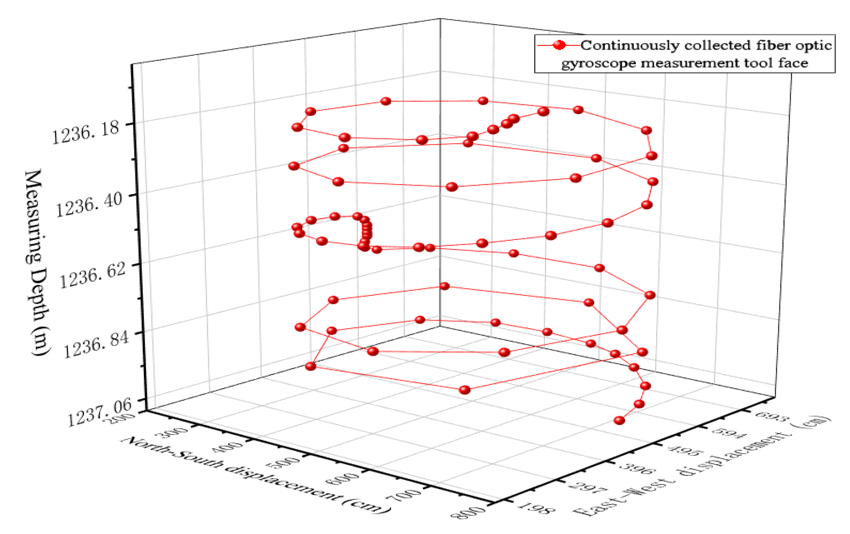
2.1. Basic Data

While performing drilling-shaft surface reconstruction, the drilling caliper data drilling trajectory data and gamma or resistivity imaging data were collected. Based on which, a 3D trajectory curve along the shaft surface was obtained. It can be seen that the geological parameters of the imaging data and the corresponding relationship with the wall surface were established. Finally, a color scheme can be added to the 3D wellbore surface reconstruction. The data measured by IMWD are used to form a ( D e p t h , I n c , A z i ) set on the wellbore axis, and then a continuous well trajectory is formed using the minimum curvature method or the minimum radius method. An ultrasonic borehole diameter sensor is used to measure the borehole diameter in real time, and the measurement point set ( Φ , L , R )   is obtained by combining the sensor measurements and ground depth data obtained by a fiber optic gyroscope, where Φ, L, and R are the measuring tool surface angle, sounding depth, and measured borehole diameter, respectively. In this methodology, the borehole diameter measurement accuracy can reach ±1 mm. The imaging data of 8, 16, or more sectors can be obtained by using gamma or resistivity imaging instruments, where the data can be represented as ( Φ , L , Gr ) and ( Φ , L , Res ) , with Gr denoting gamma data and Res denoting resistivity data.
For a real wellbore, although there are a variety of diameter changes, from a macroscopic point of view, the bore is a regular hollow cylinder structure. IMWD instruments measure the hole deviations, azimuth, caliper, natural gamma ray data, and electrical resistivity. Sensors placed on the surface or in the middle of the drill collar scan and measure the borehole wall during the drilling process Some of the measured real-time data are uploaded and stored for playback after data processing. Unlike wireline logging of the relative mean velocity measurements, due to the influence of drilling and downhole friction, the measured velocities in the radial and circumferential directions vary nonuniformly, and the measured points on the circumferential direction also vary (as shown in Figure 1). The measurement depth and tool surface of each sensor are different at the same instant, and the relative asynchronous measurement results constitute a complex of measurement parameters in chronological order. There are many challenges in the reconstruction of the wellbore surface due to the abovementioned characteristics, such as the sparsity and nonuniformity of the borehole wall measurements and the asynchronous sampling between each measurement sensor.

2.2. Problems in Current Surface Reconstruction Technologies

In the parallel contour method for surface reconstruction, discrete points on the surface are aggregated into several disjointed sections, as shown in Figure 2 [7]. Among them, some points on the surface are in point set A with m points, and some are in point set B with n points. In this method, the points on two closed contour lines are connected to form a number of triangles, and an outer surface is formed between the two contour lines. The more mature methods include the triangle method, minimum surface method, shortest diagonal method, implicit function surface method, and slice-seam method. However, these are only used if the number of points m is not too different from the number of points n. When there is a big difference between m and n, the regions of the point set with fewer points correspond to multiple edges on the point set with more points, and the constructed 3D structure becomes rough, and, in some instances, even loses the characteristics of the structure itself [8,9,10,11,12].
Another method is to use the Delaunay irregular triangulation mesh to realize the segmentation and modeling of discrete data points in space [13,14,15]. For a uniform set of spatial points, the technology of using Delaunay triangulation to form a spatial surface is relatively mature. However, for the sparse spatial point cloud on the hollow cylindrical surface, this method has difficulty constructing a smooth cylindrical surface, as shown in Figure 3. For example, in real wellbore surface scan data, due to the fast drilling process, the data points are sometimes dense, and other times sparse and uneven. When the set of points on the borehole wall is very sparse, the Delaunay subdivision may treat the sparse points on the borehole wall as holes. For the hole surface reconstruction along with the drilling borehole scan data, the wellbore formed by Delaunay triangulation is relatively rough. This method is also fairly (cannot use “more”, as we are not comparing to anything) complicated and difficult to code, and it cannot complete the task of the real-time calculation and display of changes of the surface of the drilling bore, as shown in Figure 3.
The characteristics of the wellbore measurement data are summarized as follows: (1) there is a definite central axis; (2) the borehole wall data are measured and recorded in time sequence with progressing depth; (3) the measurement data are sparse in some places and dense in others; (4) the overall shape is an irregular hollow cylinder. For wellbore surface reconstruction while drilling, the following problems must be solved: (1) The measured uneven caliper data must be interpolated to construct a relatively uniform spatial wellbore surface structure; (2) the formed surface structure can easily establish a one-to-one correspondence with gamma and resistivity imaging sector data; (3) the method needs to be simple and easily implemented by programming, which in turn would enable real-time processing and real-time display of the wellbore surface reconstruction while drilling.

3. Principle of Wellbore Surface Reconstruction Using Spiral Contour Methodology

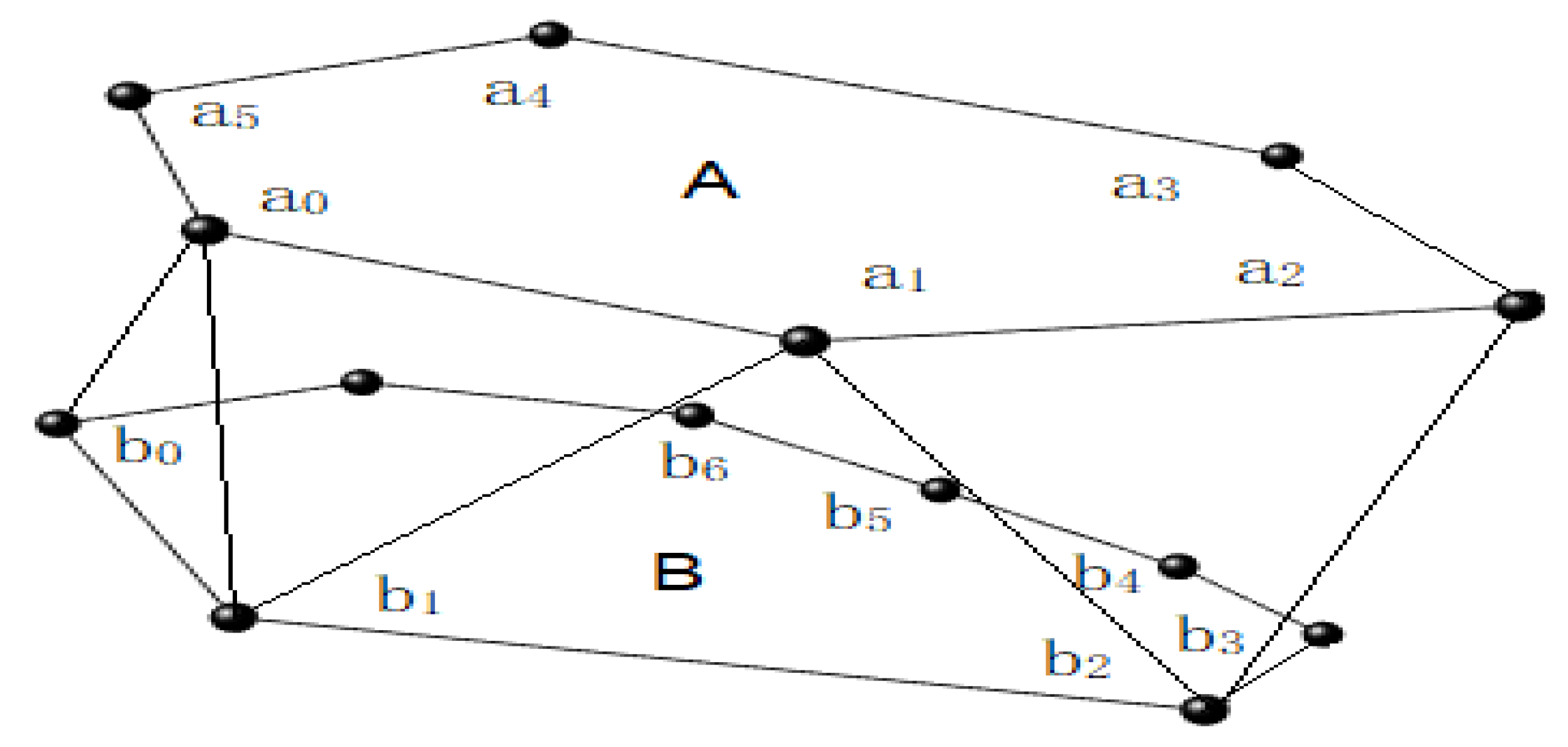
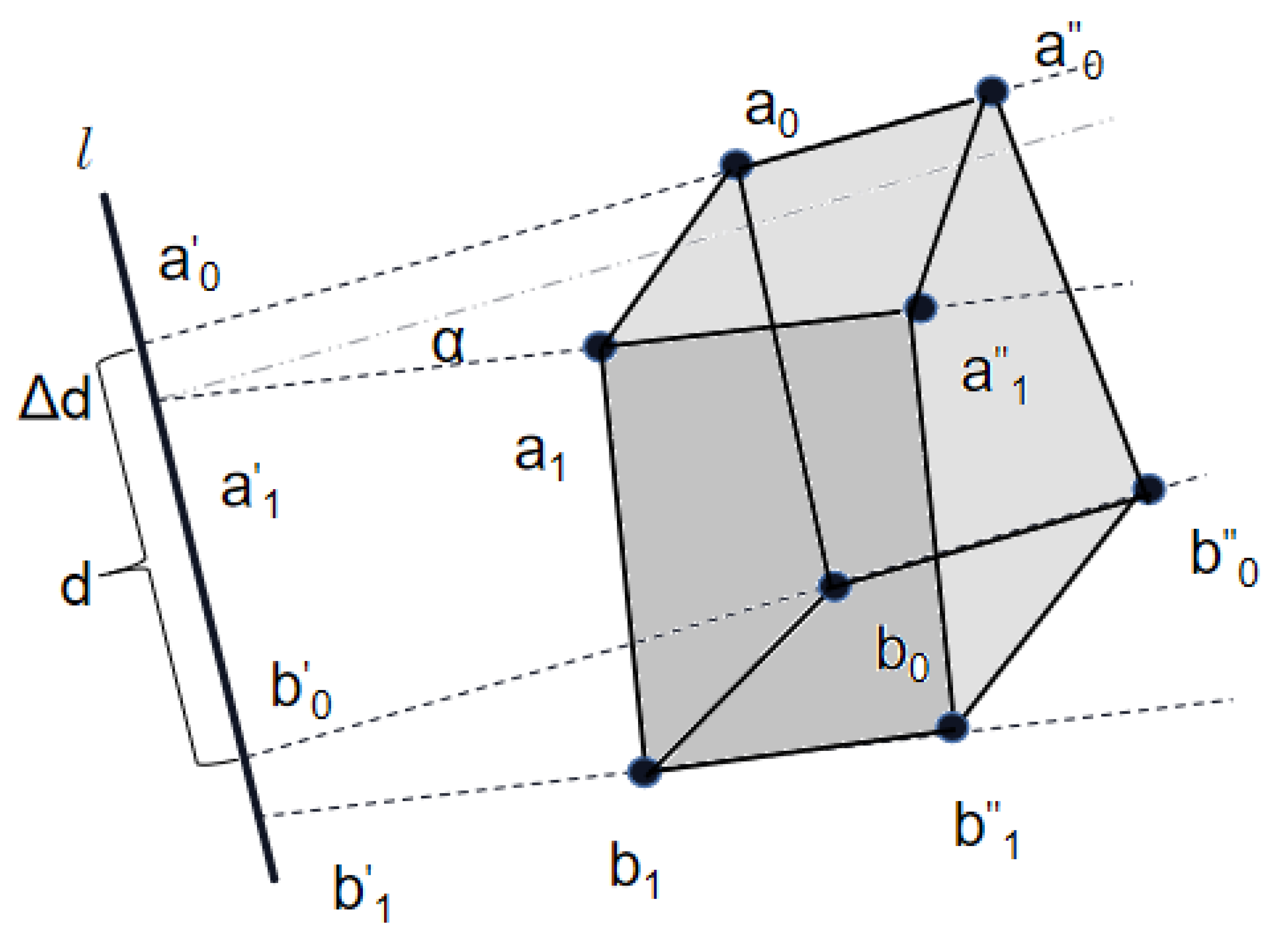
3.1. Basic Structure of Surface of Wellbore with Spiral Profile

Unlike the traditional classical parallel contour line, the discrete data points around the wellbore are sorted, and then a spiral curve around the wellbore axis is formed. Relative to the original measured helix, the data points and pitch on its circumference become relatively uniform. Two points on adjacent helices are selected to construct a quadrilateral as the basic element (Figure 4). Relevant quadrilateral sequences are then successively established around the wellbore to establish the entire surface of the wellbore. Based on the direction of the normal vector crossing the surface of the wellbore from the axis, the quadrilaterals are ordered counterclockwise in accordance with the right hand rule at the point a 0 , a 1 , b 1 , b 0 . The corresponding data at this point are ( Φ a 0 , L a 0 , R a 0 ; Φ a 1 , L a 1 , R a 1 ; Φ b 1 , L b 1 , R b 1 ; Φ b 0 , L b 0 , R b 0 ) , where Φ , L , and R are the tool surface angle, measurements depth, and wellbore diameter at a particular point.
The quadrilateral obeys the following rules on the spiral contour:
  • Rule 1
On two adjacent spiral lines, the included angle of rotation around the axis line from a 0 to a 1 is the same as the included angle of the rotation around the axis line from b 0 to b 1 , with a magnitude of α , that is, the angles between adjacent points on the pitch are equal.
  • Rule 2
The projection points of a 0 , a 1 , b 1 and b 0 on the axis of the spiral are a 0 , a 1 , b 1 and b 0 . The length of the line segment a 0 a 1 between the projection of the two points a 0 and a 1 on the axis is equal to the length of the line segment b 1 b 0 between the projection points of the two points b 0 and b 1 on the axis, where the length is Δ d .
  • Rule 3
The length of the line segment a 0 b 0 between the projection points of the two points a 0 and b 0 on the axis is equal to the length of the line segment a 1 b 1 between the projection points of the two points a 1 and b 1 on the axis, where the length is d . Thus, the pitches of the two adjacent spirals are equal.
  • Rule 4
The division of the wellbore is as follows, where K is the number of sectors evenly divided by the wellbore.
360 α = d Δ d = K ,

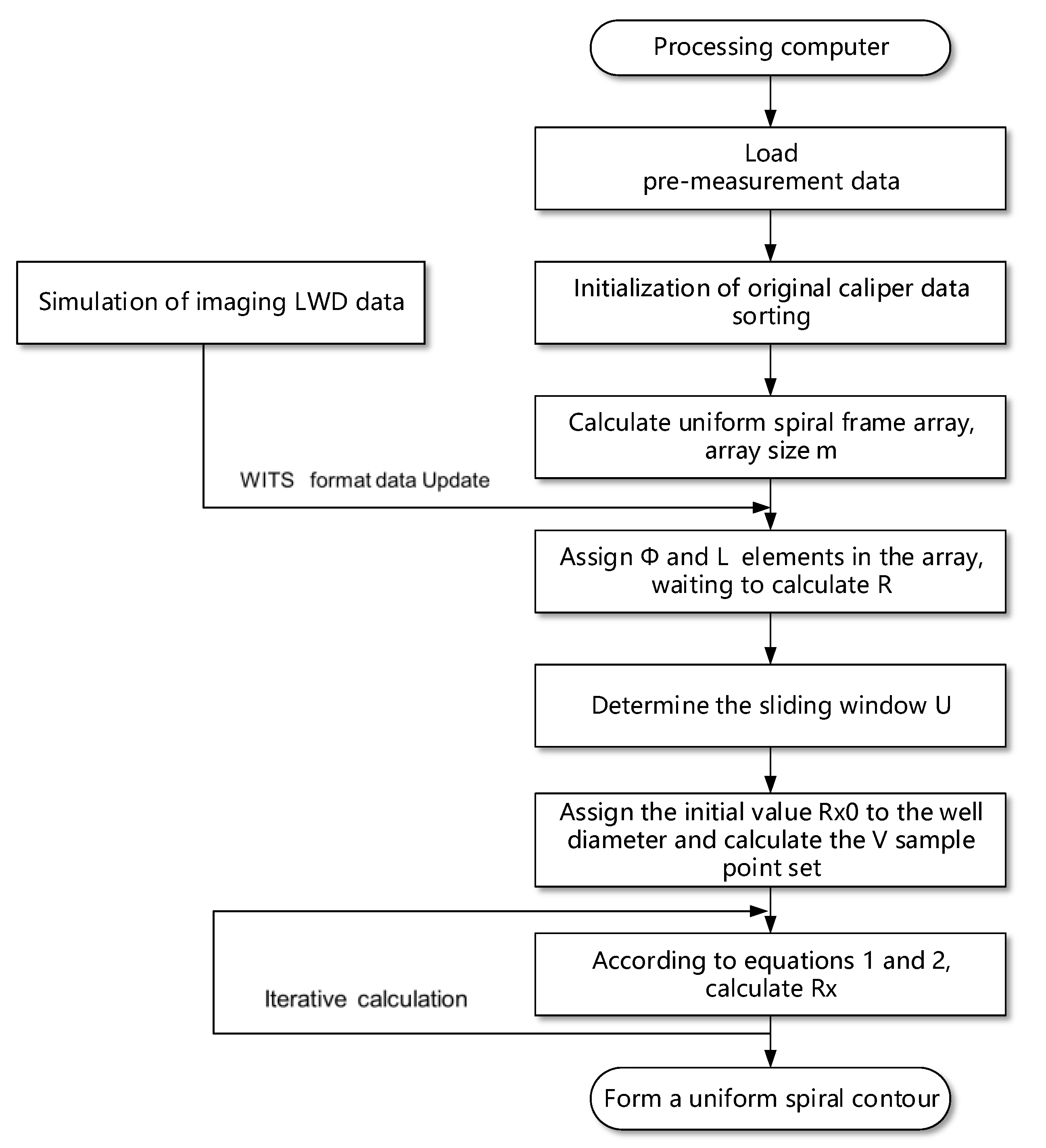
3.2. Modeling Steps for Wellbore Surface Structure Reconstruction Using Spiral Profile

3.2.1. Data Organization

First, the measured well diameter data are preprocessed and sorted in order of increasing time and depth. The redundant data are eliminated to form a point set consisting of the measurement angle, measurement depth, and ultrasonic well diameter ( Φ 1 , L 1 , R 1 ; Φ 2 , L 2 , R 2 ; ; Φ n , L n , R n ) . Thus, an ordered set of points in space with a rotation angle period of 360° is obtained, arranged by increasing angle and depth.

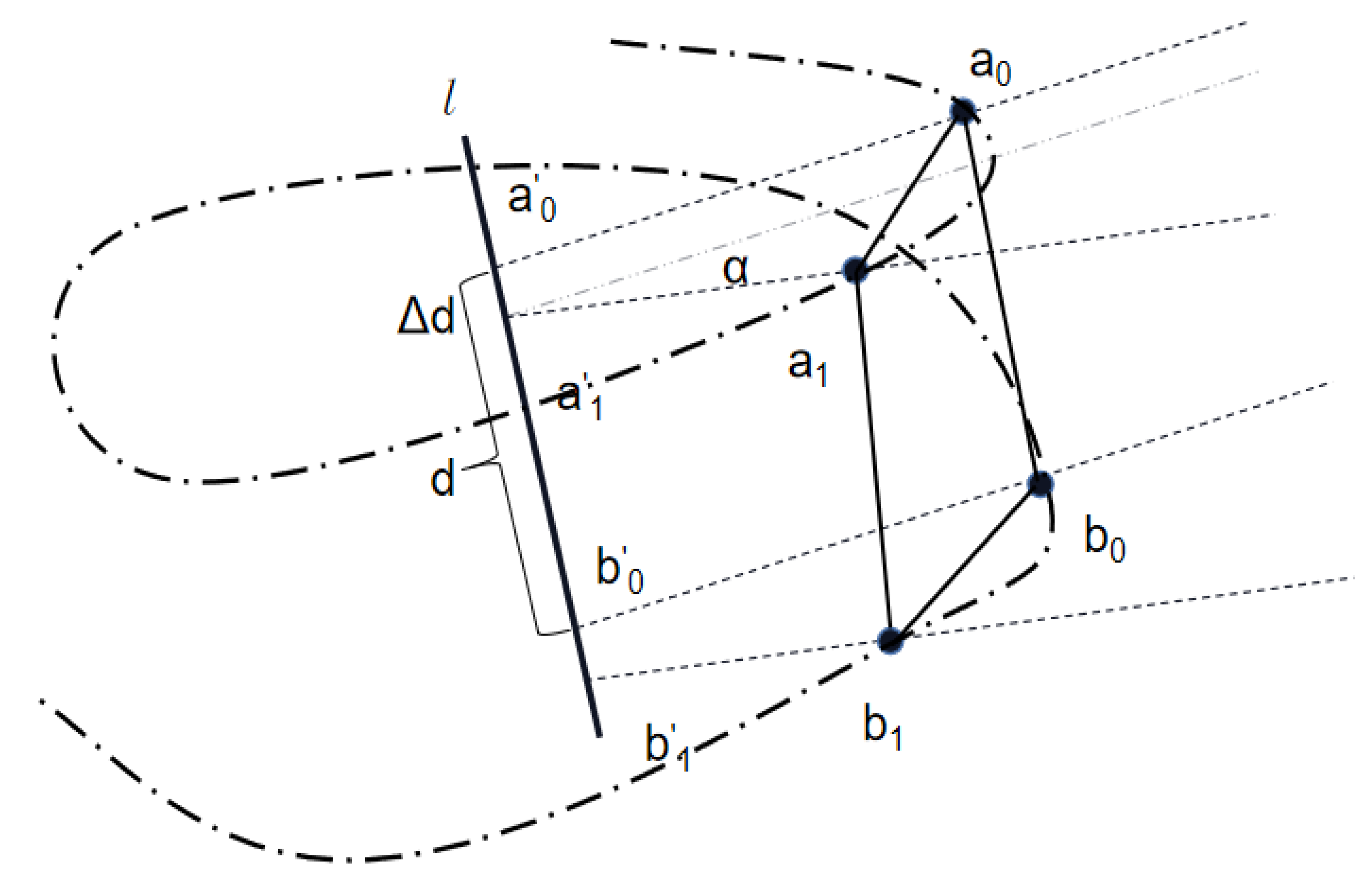
3.2.2. Angle and Pitch Homogenization

The above point sets have uneven angles, uneven depths, and uneven data density and sparsity. Direct triangulation leads to large differences in the sizes of the triangular surfaces, and the reconstructed surface is rough and irregular. To form a relatively smooth wellbore structure and establish a uniform surface, it is necessary to process the spatial dataset to form a relatively regular spiral. The spatial point set after the original scanning arrangement is transformed into a helical point set with uniform rotation angle and drilling depth:
( Φ 0 , L 0 , R 0 ; Φ 0 + α , L 0 + Δ d , R 1 ; ; Φ 0 + m × α , L 0 + m × Δ d , R m ) ,
where Φ 0 is the starting angle of the well diameter scan, L 0 is the starting depth of the well diameter scan, α is the increment of the angle in the scanning direction, and Δ d is the increment of the depth.
The transformed helix uniformly changes by an angle α , and the 360° turn of a helix is uniformly divided into several segmentation angles. Through the above steps, the data are mapped to the evenly segmented sector surfaces of the well shaft. When divided into K sectors, α is equal to 360 / K . After transformation, the helix increases uniformly according to the step length Δ d , where Δ d = P i t c h / K , and the pitch can be selected as required (e.g., 0.05, 0.1, or 0.125 m) Corresponding to the wellbore with a fixed measurement section length L , the winding number of the helix is also fixed, and the value is depth/pitch. When the depth of the wellbore to be treated is determined, the number of spatial point sets of helices formed is also determined as follows:
m = K × Depth Pitch ,

3.3. Iterative Cylindrical Space Surface Inverse Distance Interpolation Algorithm

There are three elements in the uniform helical point concentration described above: depth, angle, and well diameter ( Φ x , L x , R x ) . The angle and depth ( Φ x and L x , respectively) of each point in the homogenized point set are known quantities, and only interpolation is needed for the well diameter R x . The T-spline, B-spline, Kriging, and other methods are used to study the advantages and disadvantages of spatial point interpolation [16,17,18,19,20], but in terms of the cylindrical shape interpolation and computational efficiency, the inverse distance weighted interpolation has good properties [21,22,23]. In this study, the surface inverse distance weighted spatial interpolation method was used to determine the value of the well diameter on the homogeneous helix. First, some of the original measurement points closest to the interpolation point are selected to establish the sample space U. The distance between the interpolation point and each sample is calculated to sort the original sample space U. The closest points are then selected as the final impact sample V of the interpolation, and the distance is calculated (using Equation (4), below). It is assumed that the sample points in the space V have some influence on the interpolation point. However, with the increase in the distance, the influence is gradually reduced. The influences of different sample points accumulate to obtain the final value (using Equation (5), below), and the final value is calculated as follows:
d i = ( ( Φ x Φ i ) × 2 × π × R x 0 180 ) 2 + ( L x L i ) 2 ,
R x = i = 1 V 1 d i i = 1 V 1 d i × R i ,
where R x is the well diameter value obtained by interpolation, L x is the depth at the insertion point, Φ x is the tool surface angle at the point to be inserted, π is the well-known irrational number, L i is the depth of each sample point, and Φ i is the tool surface angle of each sample point.

3.3.1. Data Preprocessing and Acquisition of Sliding Window

First, the measured caliper data were preprocessed, the redundant data were eliminated, and the sequence was sorted in the order of increasing time and depth to obtain ( Φ 1 , L 1 , R 1 ; Φ 2 , L 2 , R 2 ; ; Φ n , L n , R n ) . The sample space point set was initialized, the previous sequence of the original measurement sequence was assigned to a sliding window to obtain the sequence ( Φ 1 + w , L 1 + w , R 1 + w ; Φ 2 + w , L 2 + w , R 2 + w ; ; Φ U + w , L U + w , R U + w ) , with w = 0 at this time. When the depth of the insertion point L x changed, where L x L U + U / 2 , the sample window U slides along the original sample space in the order of increasing W until L x < L U + U / 2 , and a new sample window is obtained, where 0 < w n U / 2 . This method continuously slides along the original sample, based on the size of the point to be interpolated, and forms a reduced sampling sample space around different point sets U obtained by the point to be interpolated ( Φ x , L x , R x ) .

3.3.2. Sort Point Set in the Sliding Window to Obtain the Final Calculation Sample

The above sliding window process is continued. The initial value R x 0 of the radius of the point to be inserted is set as the radius of the drill, R x 0 is equal to the radius of the drill, and the set of points to be inserted and initialized is ( Φ x , L x , R x 0 ) . The distance d 1 , d 2 , , d U from the sample space point of the original sliding window U to the point to be interpolated is calculated using Equation (4). The points are sorted based on their distance to obtain the closest distance sample space V as the final calculation sample point set, which is ( Φ 1 , L 1 , R 1 ; Φ 2 , L 2 , R 2 ; ; Φ V , L V , R V ) . For the initial assignment of the point to be inserted, R x 1 is calculated using Equation (5).

3.3.3. Iterative Calculation of Caliper of Insertion Point

Since the purpose of the spatial sorting in the previous step was to assign an initial value R x 0 to the value to be inserted, the result of the sorting did not consider the influence of surrounding factors. R x 1 calculated in the first step is affected by the value of the surrounding well diameter, which is close to the final interpolation result. Therefore, the distance between the interpolation point and the point in the sliding window U should be recalculated based on the new point ( Φ x , L x , R x 1 ) , and a new point set V should be obtained by reordering. The calculation procedure in Section 3.2 is repeated. A new caliper value R x 2 is obtained, and the first caliper calculation iteration is completed. The above cycle is continued to obtain R x 3 , R x 4 , and so on in turn, and the borehole diameter gradually approaches the interpolation accuracy limit, which is limited by the sampling accuracy (when the data is dense, this point is directly assigned the real sampling value). Based on this method, R x can be finally be obtained after several iterations. The number of iterations is affected by the sample value, which will be further discussed in the following experiments.

3.4. Adjustment Method of Surface of Wellbore after Data Update

3.4.1. Data Update

For imaging measurements while drilling, the amount of data of the wellbore is constantly increasing with the drilling process. For this reason, it is necessary to constantly update the wellbore model. Compared with the global data update and calculation required for traditional spatial interpolation and reconstruction, the method in this article is relatively simple, with fewer calculation steps, and the updating method is as follows.
First, it is necessary to judge whether the updated point set is within the range of the next spatial quadrilateral and to process it according to the following criterion:
{ ( Φ , L ) ( Φ 0 + ( m + 1 ) × α , L 0 + ( m + 1 ) × Δ d ) - - - - - - - - - - - - D i r e c t   c o n n e c t i o n ( Φ , L ) ( Φ 0 + ( m + 1 ) × α , L 0 + ( m + 1 ) × Δ d ) - - - - - - - - - - - - C o n n e c t   a f t e r   i n t e r p o l a t i o n ,
When the real-time added data is in the next grid, a direct connection can be adopted to display the new data point on the graph in real time. When the real-time data cross the next increasing quadrilateral, the number of quadrilaterals can be increased accordingly. Finally, the value is not in the spatial quadrilateral, and then interpolation is performed. The new sample value is used to update the sliding window presented in Section 3.3.1 according to the first-in/first-out principle, so that the sliding window maintains the latest U sample values. The new spiral point is then calculated based on the increase in the depth and angle. The quantity m is then calculated according to the methods presented in Section 3.3.2 and Section 3.3.3 to obtain the supplementary points on the new spatial spiral, and the newly added measurement points to the existing sequential spiral are updated.

3.4.2. Point Interference Reconstruction

Because the drilling time is too fast and the scan point set on the borehole wall is too sparse, to review and obtain important location information, an engineer must operate the IMWD tool lift to scan the wellbore for supplemental testing. In this case, it is necessary to recalculate and update the supplementary test part. As stated above, for the data point set of the determined measurement depth, when α and Δ d are determined, the number of data points on the unique homogenized space spiral can be obtained. For the supplementary measurement data, the depth does not increase, nor does the number of points on the spatial spiral. The data for the supplementary measurements are only updated for the interpolation point set that has been calculated. Based on the data that have been supplemented, we divide it into the range of influence on the wellbore including the supplementary data points, which are in the angle range of i × α and the depth range of j × Δ d . There are i × j constant points on the spiral line of the uniform space in this range. To obtain the data points of the supplementary measurements, the spiral interpolation steps presented in Section 3.3.1, Section 3.3.2, Section 3.3.3 are used. The sliding window U and the calculation sample window V are selected again. The i × j points in the affected angle range i × α and depth range j × Δ d are updated, and the set of points that are not affected in other spaces remain unchanged.
The above method does not require overall intervention, but only partial updates, and the calculation effect is high. The update and interpolation calculation can be completed on a field collection computer in real time.

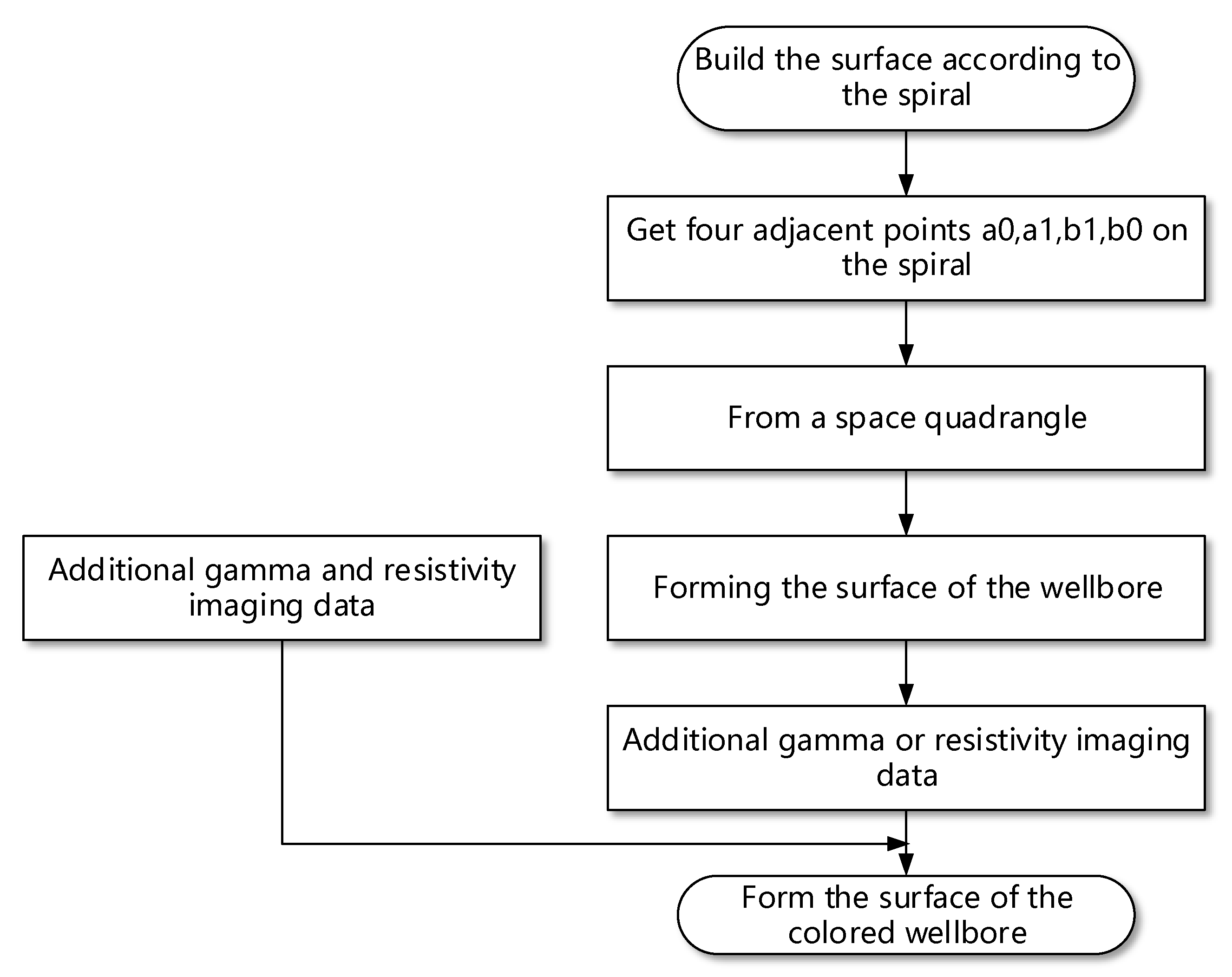
3.5. Extension from Surface to Volume

For wellbore modeling, it is also necessary to establish a wellbore structure with a certain thickness, which is used to describe the shape of the mud cake on the well wall and the geological structure for deep exploration. For example, the depths of the deep, medium, and shallow measurements of the azimuth imaging resistivity are different, reflecting the different thicknesses of the reservoir and formation structure of the extension part of the wellbore, and the subsequent formation profile can be measured. In this way, it is necessary to expand the surface of the wellbore to form an epitaxial structure that wraps the surface of the wellbore and to expand the inner surface structure of the wellbore to a hollow cylindrical structure surrounding the axis of the wellbore.
To reconstruct the spiral contour line with the surface of the drilling barrel involved in this study, it is only necessary to build a new uniform spatial spiral. The hollow wellbore with a certain thickness is described by two continuous spiral lines, where each spiral line represents the surface of the thick wellbore. The structure of the basic unit of the hollow wellbore is completed by combining two spatial quadrilaterals corresponding to the two spiral lines into a spatial hexahedron. Each spatial hexahedron of the hollow cylinder structure (Figure 5) is composed of eight spatial points on two spiral lines, which are the quadrilateral point a 0 a 1 b 1 b 0 on the inner spiral line and the point a 0 a 1 b 1 b 0 on the outer spiral line. For two corresponding points on the two spirals, such as a 0 , a 1 , the tool face angles Φ a 0 and Φ a 0 are equal, and the measured depth L a 0 is equal to L a 0 . The bore diameter R a 0 corresponding to a 0 and the bore diameter R a 0 corresponding to a 0 is different. The length of the line segment a 0 a 1 is the difference between R a 0 and R a 0 , which is the thickness of the wellbore structure at that location. The use of two spatial spirals can form a wellbore structure with a certain thickness.

3.6. Method for Wellbore Attribute Assignment

Typically, images obtained while drilling are ordered based on the depth of the measurements, and 8, 16, 32, or 128 curves are formed in a sector-by-sector manner to represent the property changes around the wellbore. In existing engineering applications, the imaging data during drilling are generally expanded along an angle into a two-dimensional map, and different colors are used to represent the changes of the data. It is difficult to understand the spatial changes of the wellbore and the trend of the formation from these images [24]. The existing spatial expansion also uses conventional three-dimensional graphics and image technology to establish the borehole surface, and rendering technology is used to add color to the surface. It is difficult to establish the correspondence between sequentially arranged imaging data while drilling and the scattered triangles on the wellbore. It becomes difficult and time-consuming to add color information for imaging while drilling in the wellbore space.
However, based on the wellbore spatial data points established in this study, each spatial quadrilateral corresponds to the depth and sector measured by imaging while drilling. The imaging data while drilling and the wellbore spatial data can establish a one-to-one correspondence between the well diameter and the measured data based on the measured depth and tool surface, forming a spatial quadrangle ( a 0 , a 1 , b 1 , b 0 , v 1 , v 2 ) with additional measurements or analysis attribute values, e.g., v 1 and v 2 , which represent different IMWD properties, such as gamma and resistivity measurements. Using this method, it is easy to build a color 3D wellbore surface. The reconstructed surface is smooth and retains all the details of the IMWD data control points, and the measurement attributes and assignments can be quickly changed based on the different measurement attributes.

4. Experiment and Applications

To simulate the real-time processing of imaging measurement data while drilling, we first used a three-axis fiber-optic gyro while drilling to obtain the effects of the downhole measurement rotation speed and drilling time under actual drilling conditions. This working condition was attached to the ultrasonic caliper test equipment for open hole scanning in a calibrated well in the Shengli Oilfield of China, and further organized the original imaging measurement data of the well into a measurement while collecting drilling data; the resulting caliper data are shown in Figure 6. This method performed well from data preparation to the real-time reconstruction of the spiral contour line along the surface of the drilling barrel.

4.1. Experimental Conditions and Experimental Procedures

The abovementioned imaging and drilling measurement data were uploaded onto a Thinkpad T490 notebook to simulate the image acquisition process while drilling. The experimental well was drilled with a 216-mm drill bit, and the irregular radius was approximately 110 mm. A Thinkpad T590 computer was used to conduct the data calculation and display of the real-time reconstruction method results along the drilling borehole surface. The two laptops used a network cable for data exchange, and the transmission data format used the wellsite information transfer specification (WITS) protocol data format commonly used in the petroleum industry. The notebook computer T490 used for the experiments was configured for network transmission and exchange of IMWD data, and the experimental data were input to the T590 processing computer through the network cable for real-time processing. The independently developed wellbore surface real-time reconstruction software based on the method described above was installed on the computer. The computer operating system was Windows 10 Home Edition, the programming language was Visual Basic, and the data storage was binary text format.
The real-time wellbore surface reconstruction software performed data processing based on the two main software flowcharts. One flowchart illustrates the steps for processing the imaging-while-drilling measurement data to form a uniform contour line around the wellbore (Figure 7). The other flowchart illustrates the procedure of taking two points from each adjacent spiral on the homogenized spatial spiral, forming a spatial quadrilateral, and then splicing all the spatial quadrilaterals to form the inner surface of the wellbore (Figure 8).

4.2. Comparison of Spatial Interpolation Results

4.2.1. Analysis of Relationship between Sample Size and Interpolation Distance to Be Interpolated

As shown in Figure 9, the sliding window U was programmed to read data, and the value of the sliding window sample was 100. Assuming that the initial value R x 0 = 11 cm for the insertion point, the distance between the points in the sliding window were calculated using Equation (4), and the values were sorted to obtain the results shown in Figure 9. Point no. 0 is the point to be inserted on the helix, and the data points in the sliding window were sorted as no. 1–100 based on the distance between them.
Based on the method in the flow chart shown in Figure 7, the first eight sorted values in the sliding window U were selected to establish the value sample space V , and the coordinates of points on the borehole wall after interpolation were obtained through continuous iterative calculations. Figure 10 shows 20 points randomly checked during the interpolation calculation. The curves in the figure show the distance between the interpolation points and the sample space V in turn. The distances between the interpolation points and the sample space V increased in order. When V was 4, the radius of the sample surrounding the interpolation point was less than 0.5 mm, and when V was 8, the radius of the sample surrounding the interpolation point was less than 0.7 mm. The number of data points of the borehole wall collected by the IMWD ultrasonic caliper affected the accuracy of the wellbore surface reflected by the spatial helix after the interpolation calculation.

4.2.2. Comparison of Interpolation Iterations

In the interpolation process, the radius of the interpolation point was first treated with the initial value Rx0 = 11 cm, and the black line in Figure 11 represents the uniform initial value of the well diameter of each interpolation point. Four iterations were conducted according to the method shown in Section 3.3.3, and the 390 interpolation points in Figure 11 were randomly checked. The first calculation result after the initial value basically reflects the final interpolation result of the borehole wall, but there were still 15 points that needed to be further iterated. The above 390 point sets were iterated once, and it was found that only one sample still needed to be iterated. The second, third, and fourth iterations were performed, and the spatial points after interpolation were completely consistent and did not change. Thus, in most cases, interpolation calculations only require two iterations to meet the interpolation requirements, and there is no need to consume computing resources and time to perform more iterations.

4.2.3. Analysis of the Model Fit between Data and Wellbore after Interpolation

To verify the model fit between the point set on the spatial helix and the wellbore surface after interpolation, the following tests were conducted. During the interpolation process, 10 groups of data were randomly selected based on the condition that the spatial distance on the nearest sample V was <0.01 mm. At this time, it was assumed that there was an actual measurement point on the spatial helix. Therefore, the fitting relationship between the point set on the spatial helix and the wellbore surface could be obtained by comparing the well diameter Rx of the interpolation points on the calculated helix with the value of the first point set on the sampling space V . In Table 1, the second row shows the distance between the interpolation points of the ten sets of data and the nearest measured point. The third row shows the difference between the interpolation points and the nearest measured point. The fourth line shows the similarity between the interpolation point and the nearest point. The fifth line shows the diameter of the well after interpolation. The sixth to the twelfth row show the size of the well diameter corresponding to V 1 V 7 in the sample space. Table 1 shows that although the diameter of V 1 V 7 varied, the nearest V 1 determined the Rx size of the point after interpolation. The third row in the table is the difference between the corresponding diameter of V 1 and the corresponding point on the calculated spiral contour line, and the absolute value was less than 0.02 cm. This was less than the ultrasonic measurement accuracy. The fourth row of the table shows that the similarity between the difference point and the measured point was >99.5%, and the data after the difference value were close to the real measured value. Thus, when the sample values were relatively dense, the spatial helix calculated using the method proposed in this study strictly conformed to the actual wellbore size.

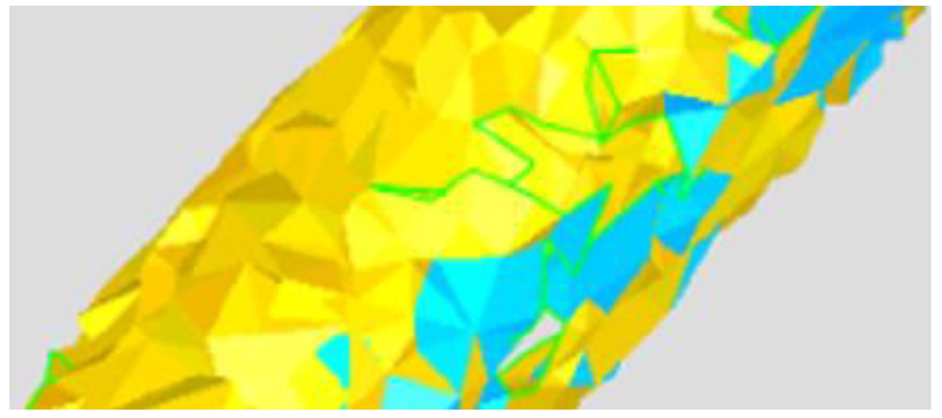
4.3. Inner Surface of Wellbore and Attribute Assignment

Based on the experiments and analysis described above, after the corresponding processing of the data points measured while drilling, the entire dataset was transformed into a continuous line around the borehole surface (Figure 12). The spatial curve strictly follows the spiral contour rules proposed in this study. After the above set of spiral points was obtained, the flow chart of the wellbore surface composed of spatial quadrilaterals was established using the uniform spiral, as shown in Figure 8, to construct the spatial quadrilateral and represent the inner surface of the wellbore.
The structure after treatment is shown in Figure 13a,b. According to the rules of spiral wellbore surface reconstruction, four adjacent spatial points were connected to form the inner surface structure of the wellbore, forming a relatively smooth surface (Figure 13a). The quadrilateral can be divided into two triangles by adding a diagonal line to each parallelogram in the clockwise direction of the drilling rotation (Figure 13b). Figure 13 was established based on a Cartesian coordinate system, in which the Z-axis represents the vertical direction of the wellbore, the X-axis represents the north–south direction displacement of the wellbore, and the Y-axis represents the east–west displacement of the wellbore, which follows the typical convention used in the oil industry.
After the completion of the wellbore quadrilateral, the reconstructed surface quadrilateral and the depth and angle (sector) of the measured data had unique properties, which corresponded to the gamma and resistivity imaging data that were also obtained while drilling. The quadrilateral was colored based on the corresponding relation by using the imaging measurement chromatography to form a relatively intuitive color wellbore spatial structure, as show in Figure 14.

4.4. Applications

Through the research of the above technology, we selected two wells for the field application of the wellbore surface reconstruction technology. Among them, the Sheng3-X5 well was located in Shengli Oilfield, China. The depth of this well was 2458 m. The applied interval was 1865 m to 1905 m, the well inclination was 48°, and the azimuth was 248°. The caliper and the gamma imaging tool while drilling were used to track the drilling. The underground measurement data was transmitted to the ground by signal transmitter, and the data transmission interval was 10 s~25 s. The computer processed the downhole data in real time; the information transmitted downhole can be processed in real time using the method of surface reconstruction of the borehole wall described in this article, the data was processed in real time using the flow chart of Figure 7 and Figure 8, and the data processing speed was less than 1 s. In the process of data processing, this method can be used to separate specific well sections for a full-scale display of rotary amplification (Figure 15), which meets the needs of geological engineers for real-time analysis.
The Peng154-P1 well was located in Sichuan Province, China. The depth of the well was 3085 m, and the application interval was 2480 to 2530 m. This section had a deviation of 38° to 44° and an azimuth of 52°. The caliper and the gamma imaging tool while drilling were also used to track the drilling. This section used the method of this article to construct a borehole wall model in real time, and used gamma chromatograms of different colors to represent changes in lithology. In this case, the formation with low gamma was found at 2510 m in time, and compared with other information to identify the oil layer; it can be seen that real-time well wall reconstruction provides a very friendly interactive method for geological analysis and identification (Figure 16).

5. Conclusions and Discussion

In this study, a method to reconstruct the surface of a wellbore using a continuous spatial helical curve is presented, and a rule for constructing quadrilateral elements to represent the wellbore surface is developed. Using this method, a relatively smooth wellbore surface was reconstructed using the multi-source discrete data of the trajectory, diameter, and wellbore properties measured while drilling, which is of great value for the real-time evaluation of the drilling risk and geologically guided decision-making in drilling engineering. This method has the following advantages:
(1)
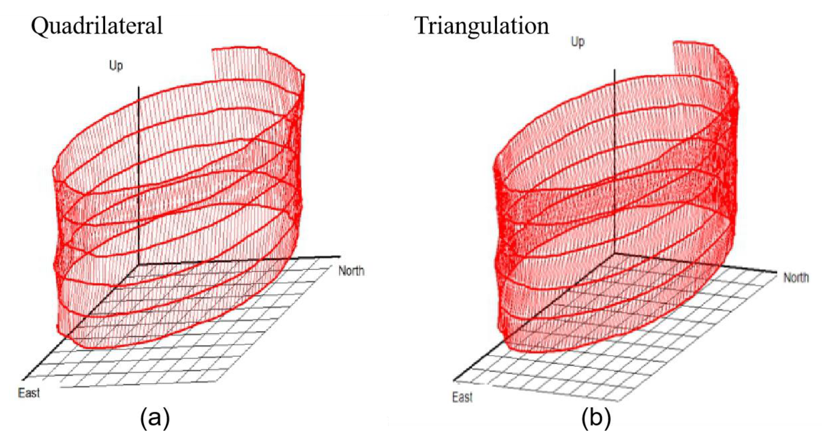
The method proposed in this paper reconstructs the solid wellbore surface into a spiral curve with continuous and uniform spacing. The four adjacent points of the upper and lower pitch form a quadrilateral to form the wellbore surface, which could be extended to describe the wellbore surface with a certain thickness.
(2)
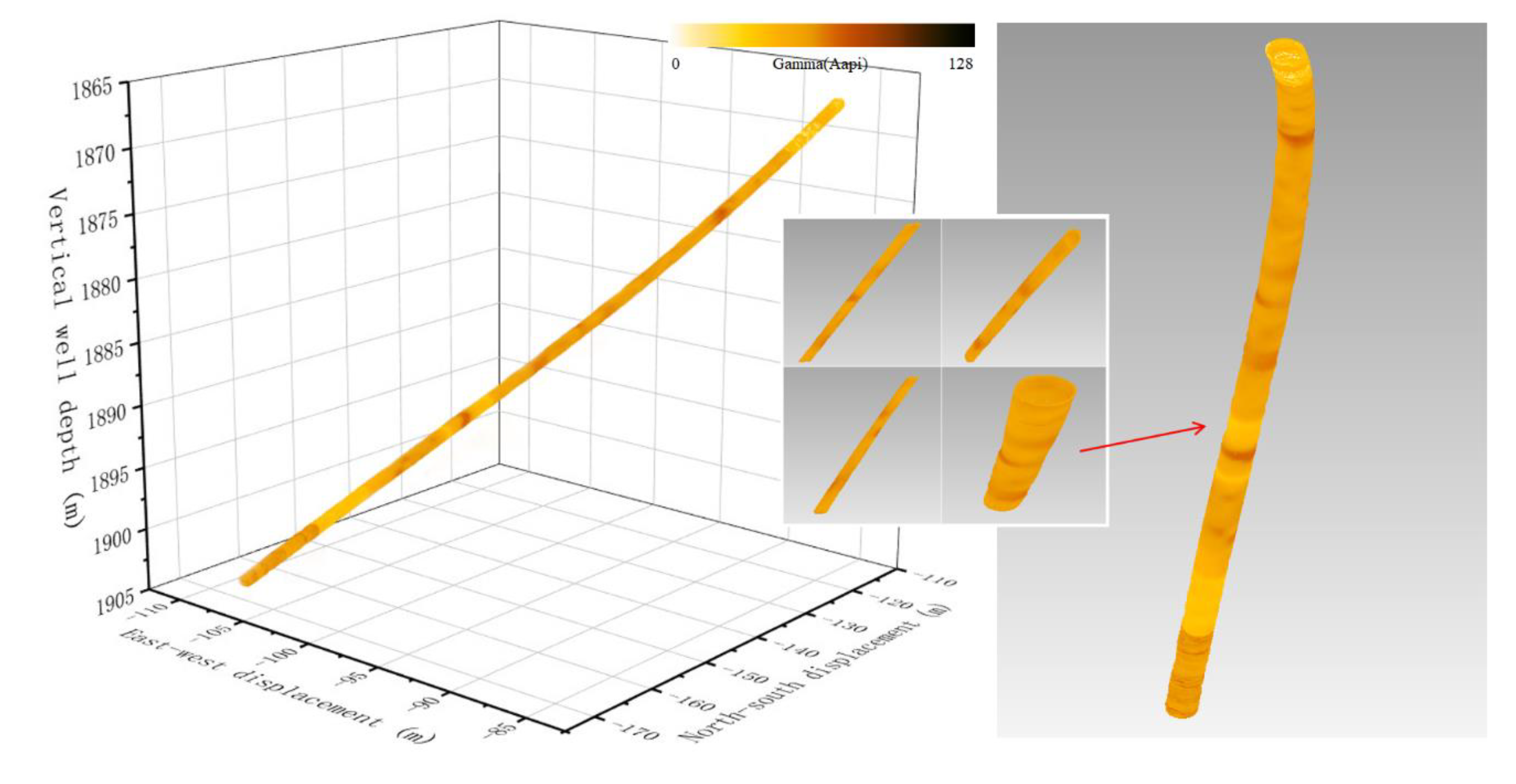
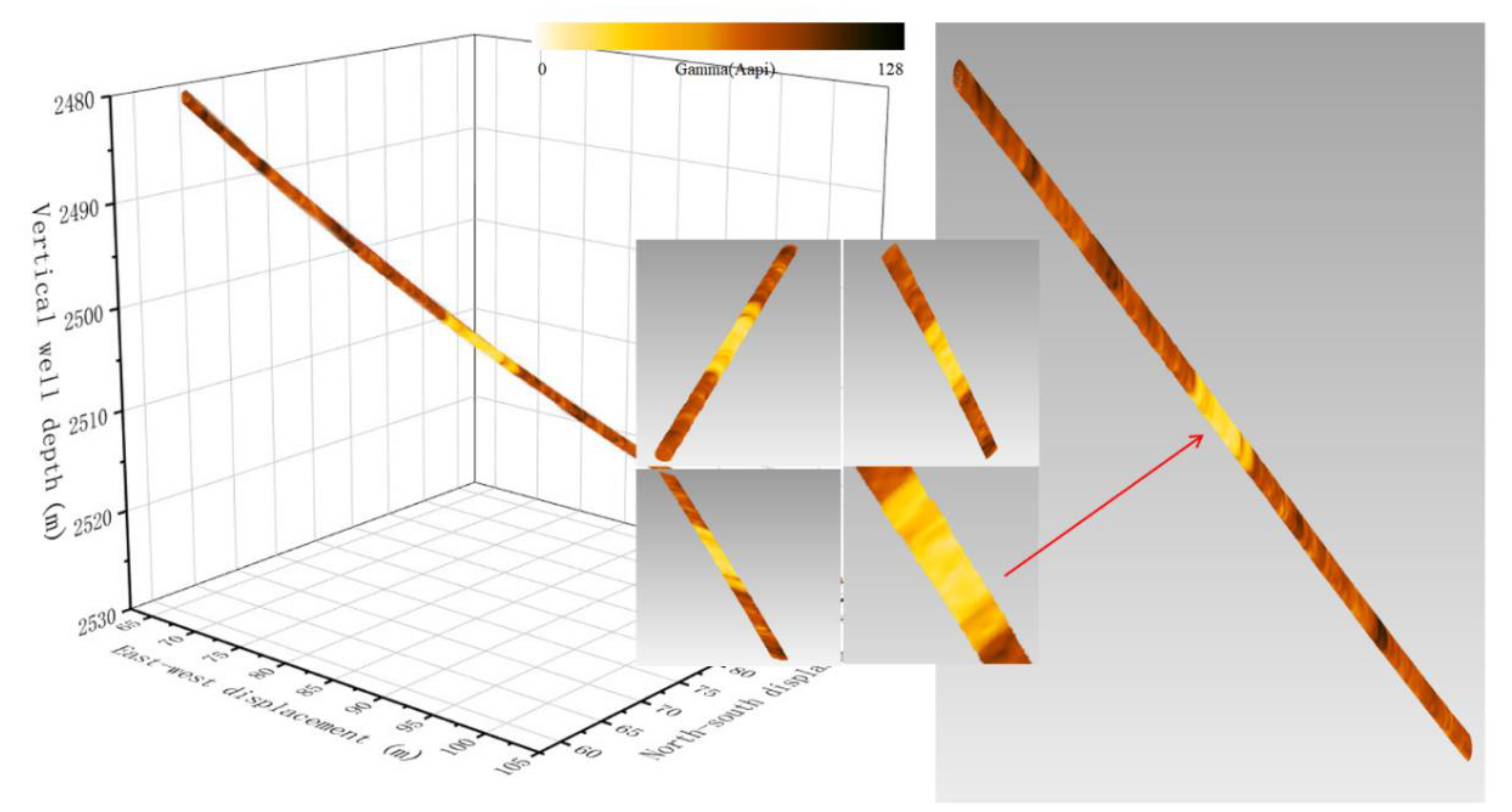
The improved inverse distance weighted interpolation method takes into account the influence of the wellbore shape on the caliper interpolation. A sliding window was used to reduce computation volume. The wellbore surface was reconstructed with high similarity to the actual measurement data. The measured data could be updated in real time, data could be stored, and the calculation efficiency was high.
(3)
The spatial quadrilaterals were further constructed to form triangular facets. The existing file architecture and display software could be used to visualize and store the data points.
(4)
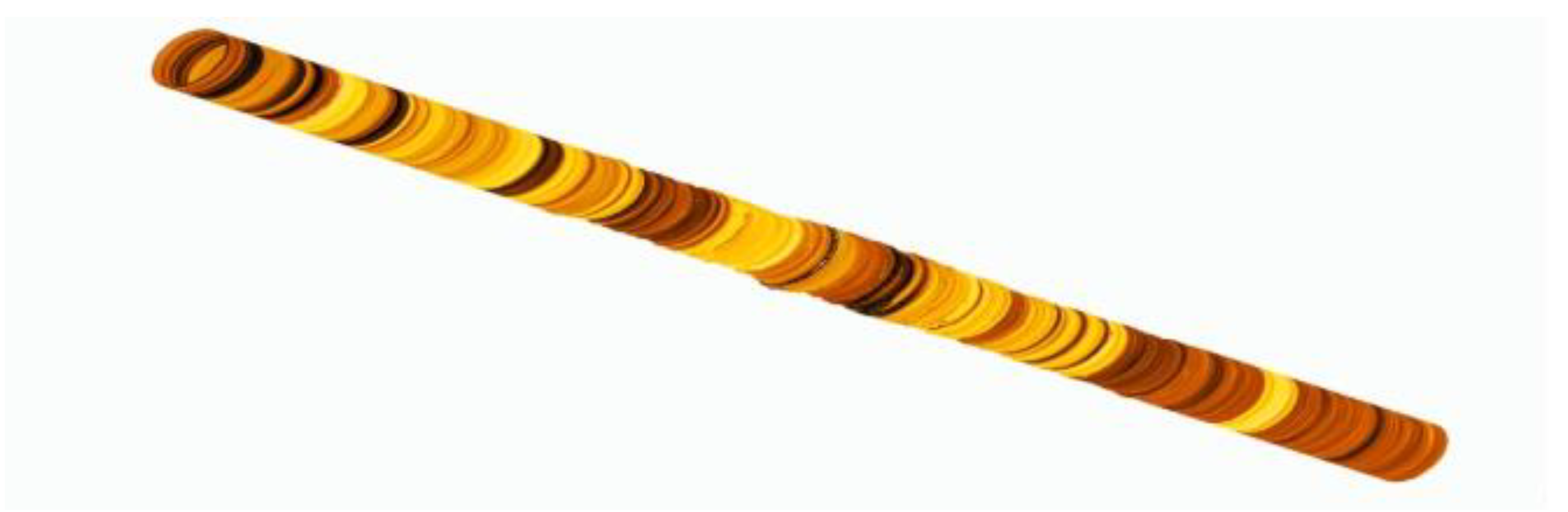
The constructed space quadrilateral and partial hexahedron corresponded to the sector data measured by imaging while drilling, which is convenient for adding geological properties.
This method can be used to calculate and display the wellbore structure properties in real time using a portable computer on the engineering site, whether for the data transmitted in real time or stored. However, the degree to which the established wellbore surface shape matches that of the real wellbore depends on a relatively uniform downhole rotation measurement and data uploading. A small amount of data while drilling still distorts the wellbore shape. Further optimization of the sensor measurement frequency and speeding up the transmission of the downhole information to the surface is required.

Author Contributions

All the authors made contributions to this work. This concept was originally proposed by R.W. and H.L. H.L. proposed the scheme, developed the algorithms and software, completed the experiment, and wrote the manuscript. All authors have read and agreed to the published version of the manuscript.

Funding

This research was funded by the National Science and Technology Major Project of China, grant number 2016X05011-002.

Institutional Review Board Statement

Not applicable.

Informed Consent Statement

Not applicable.

Data Availability Statement

The study did not report any data.

Acknowledgments

The first author is very grateful to his teacher Ruihe Wang for providing guidance and helping in the research process. Wang reviewed and revised the main structure of the article in detail. The authors are very grateful to Genlu Huang for providing guidance on the structure of the article. The authors thank Qifeng Sun for useful discussions on the experimental analysis and methods. The authors thank Lu Wang for useful discussion on writing the article.

Conflicts of Interest

The authors declare no conflict of interest.

References

  1. Prammer, M.; Morys, M.; Kizhnik, S. Field testing of an advanced LWD imaging resistivity tool. In Proceedings of the SPWLA 48th Annual Logging Symposium, Society of Petrophysicists and Well-Log Analysts, London, UK, 3–6 June 2007. [Google Scholar]
  2. Finlay, S.; Omeragic, D.; Thiel, M.; Farnoosh, N.; Denichou, J.; Viandante, M. First Use of Ultra-Deep Resistivity 2D Deep Azimuthal Images to Identify Reservoir Sweep in a Mature Waterflood of Al-Shaheen Field. In Proceedings of the IOR 2019–20th European Symposium on Improved Oil Recovery, Pau, France, 8–10 April 2019; Volume 2019. [Google Scholar]
  3. Pickering, J.G.; Sengupta, S. Achieving Digital Oilfield Competency. In Proceedings of the SPE Middle East Intelligent Energy Conference and Exhibition, Manama, Bahrain, 28–30 October 2013. [Google Scholar]
  4. Rommetveit, R.; Bjorkevoll, K.S.; Halsey, G.W.; Fjar, E.; Odegaard, S.I.; Herbert, M.C.; Sandve, O.; Larsen, B. e-Drilling: A System for Real-Time Drilling Simulation, 3D Visualization and Control. In Proceedings of the SPE Gulf Coast Section 2008 Digital Energy Conference and Exhibition, Houston, TX, USA, 11–12 April 2007. [Google Scholar]
  5. Rommetveit, R.; Bjorkevoll, K.S.; Odegaard, S.I.; Herbert, M.C.; Halsey, G.W. Automatic Real-Time Drilling Supervision, Simulation, 3D Visualization, and Diagnosis on Ekofisk. In Proceedings of the IADC/SPE Drilling Conference, Orlando, FL, USA, 4–6 March 2008. [Google Scholar]
  6. Han, R.; Ashok, P.; Pryor, M.; Van Oort, E. Real-Time 3D Computer Vision Shape Analysis of Cuttings and Cavings; Society of Petroleum Engineers (SPE): Houston, TX, USA, 2018. [Google Scholar]
  7. Keppel, E. Approximating Complex Surfaces by Triangulation of Contour Lines. IBM J. Res. Dev. 1975, 19, 2–11. [Google Scholar] [CrossRef]
  8. Mackay, D. Robust Contour Based Surface Reconstruction Algorithms for Applications in Medical Imaging. Master’s Thesis, University of Canterbury, Christchurch, New Zealand, 2019. [Google Scholar]
  9. Villard, B.; Grau, V.; Zacur, E. Surface Mesh Reconstruction from Cardiac MRI Contours. J. Imaging 2018, 4, 16. [Google Scholar] [CrossRef] [Green Version]
  10. Holloway, M.; Grimm, C.; Ju, T. Template-based surface reconstruction from cross-sections. Comput. Graph. 2016, 58, 84–91. [Google Scholar] [CrossRef] [Green Version]
  11. Liu, L.; Bajaj, C.; Deasy, J.O.; Low, D.A.; Ju, T. Surface reconstruction from non-parallel curve networks. Comput. Graph. Forum 2008, 27, 155–163. [Google Scholar] [CrossRef] [PubMed] [Green Version]
  12. Bermano, A.; Vaxman, A.; Gotsman, C. Online reconstruction of 3D objects from arbitrary cross-sections. ACM Trans. Graph. 2011, 30, 1–11. [Google Scholar] [CrossRef] [Green Version]
  13. Lhuillier, M. Surface reconstruction from a sparse point cloud by enforcing visibility consistency and topology con-straints. Comput. Vis. Image Underst. 2018, 175, 52–71. [Google Scholar] [CrossRef] [Green Version]
  14. Beaufort, P.A.; Geuzaine, C.; Remacle, J.F. Automatic surface mesh generation for discrete models—A complete and automatic pipeline based on reparametrization. J. Comput. Phys. 2020, 417, 109575. [Google Scholar] [CrossRef]
  15. Berger, M.; Tagliasacchi, A.; Seversky, L.M.; Alliez, P.; Guennebaud, G.; Levine, J.A.; Sharf, A.; Silva, C.T. A survey of surface reconstruction from point clouds. Graph. Forum 2017, 36, 301–329. [Google Scholar]
  16. Asthana, V.; Bhatt, A.D. G1 continuous bifurcating and multi-bifurcating surface generation with B-splines. Comput. Des. Appl. 2016, 14, 95–106. [Google Scholar] [CrossRef] [Green Version]
  17. Ginnis, A.I.; Kostas, K.V.; Kaklis, P.D. Construction of smooth branching surfaces using T-splines. Comput. Aided Des. 2017, 92, 22–32. [Google Scholar] [CrossRef] [Green Version]
  18. Ikechukwu, M.N.; Ebinne, E.; Idorenyin, U.; Raphael, N.I. Accuracy Assessment and Comparative Analysis of IDW, Spline and Kriging in Spatial Interpolation of Landform (Topography): An Experimental Study. J. Geogr. Inf. Syst. 2017, 9, 354–371. [Google Scholar] [CrossRef] [Green Version]
  19. Calcagno, P.; Chilès, J.P.; Courrioux, G.; Guillen, A. Geological modelling from field data and geological knowledge: Part I. Modelling method cou-pling 3D potential-field interpolation and geological rules. Phys. Earth Planet. Inter. 2008, 171, 147–157. [Google Scholar] [CrossRef]
  20. Mužík, J.; Vondrackova, T.; Sitányiová, D.; Plachy, J.; Nývlt, V. Creation of 3D Geological Models Using Interpolation Methods for Numerical Modelling. Procedia Earth Planet. Sci. 2015, 15, 25–30. [Google Scholar] [CrossRef] [Green Version]
  21. Dhamodaran, S.; Lakshmi, M. Comparative analysis of spatial interpolation with climatic changes using inverse dis-tance method. J. Ambient Intell. Humaniz. Comput. 2020, 1–10. [Google Scholar] [CrossRef]
  22. Cevik, N. A dynamic inverse distance weighting-based local face descriptor. Multimed. Tools Appl. 2020, 1–16. [Google Scholar] [CrossRef]
  23. Dag, A.; Ozdemir, A.C. A Comparative Study for 3D Surface Modeling of Coal Deposit by Spatial Interpolation Approaches. Resour. Geol. 2013, 63, 394–403. [Google Scholar] [CrossRef] [Green Version]
  24. Zhang, Q.; Zhu, H. Collaborative 3D geological modeling analysis based on multi-source data standard. Eng. Geol. 2018, 246, 233–244. [Google Scholar] [CrossRef]
Figure 1. Measuring tool surface for downhole recording.
Energies 14 00291 g001
Figure 2. Schematic modeling of parallel contour lines.
Energies 14 00291 g002
Figure 3. Wellbore surface constructed by Delaunay irregular triangulation mesh.
Energies 14 00291 g003
Figure 4. Four points on the spiral contour line constitute a quadrilateral in space.
Energies 14 00291 g004
Figure 5. Spatial quadrilateral extends to the hexahedron.
Energies 14 00291 g005
Figure 6. Caliper data obtained by scanning an open hole.
Energies 14 00291 g006
Figure 7. Flow chart for establishing a uniform shaft wall spiral.
Energies 14 00291 g007
Figure 8. Flow chart of surface reconstruction and attach attributes.
Energies 14 00291 g008
Figure 9. Distance between the insertion point and the point inside the window U.
Energies 14 00291 g009
Figure 10. Distance between the insertion point and the point in sample space V.
Energies 14 00291 g010
Figure 11. Relationship between interpolation and multiple iterations.
Energies 14 00291 g011
Figure 12. Wellbore formed by uniform contour lines obtained after processing.
Energies 14 00291 g012
Figure 13. The surface of a wellbore consisting of a quadrilateral (triangle) in space.
Energies 14 00291 g013
Figure 14. Three-dimensional wellbore with additional gamma imaging data.
Energies 14 00291 g014
Figure 15. Real-time 3D wellbore structure of the Sheng3-X5 well.
Energies 14 00291 g015
Figure 16. Real-time 3D wellbore structure of the Peng154-p1 well.
Energies 14 00291 g016
Table 1. Comparison of interpolation approximation.
PropertyTest 1Test 2Test 3Test 4Test 5Test 6Test 7Test 8Test 9Test 10Units
Distance0.000510.000270.00020.000550.000820.000230.000350.000740.000630.0008cm
Results compared0.01675−0.00044−0.017120.01492−0.00412−0.00512−0.00720.035170.0014−0.02493
Similarity99.844%99.996%99.847%99.860%99.963%99.954%99.936%99.670%99.987%99.779%
Rx10.744311.1580911.1908210.6631111.2429811.1283211.3206710.7087111.1658211.23907cm
V110.7275511.1585311.2079410.6481911.247111.1334411.3278710.6735411.1644211.264cm
V211.140111.1573811.0072311.0138911.199110.8677110.8958711.2076811.1644210.82163cm
V310.7898911.1279410.7279411.1806711.2645110.793611.1377911.3223711.2637410.82906cm
V410.6991410.8326410.615311.1965411.0828811.179910.7655711.3360611.1545611.22125cm
V511.0329610.7146210.7120610.8341810.6609910.6609910.7005410.8304610.6503711.1223cm
V610.7984610.7397110.7202610.78411.151110.9699811.1828511.0493410.7326710.77517cm
V710.8367410.6577910.6617611.1820811.0968311.151111.1809311.3360611.0585611.1223cm
Publisher’s Note: MDPI stays neutral with regard to jurisdictional claims in published maps and institutional affiliations.

