Examining the Effects of the Sacramento Dockless E-Bike Share on Bicycling and Driving

Fitch, Dillon T.; Mohiuddin, Hossain; Handy, Susan L.

doi:10.3390/su13010368

Open AccessArticle

Examining the Effects of the Sacramento Dockless E-Bike Share on Bicycling and Driving

by

Dillon T. Fitch

^1,*

,

Hossain Mohiuddin

¹

and

Susan L. Handy

^1,2

¹

Institute of Transportation Studies, University of California, Davis, CA 95616, USA

²

Department of Environmental Science and Policy, University of California, Davis, CA 41007, USA

^*

Author to whom correspondence should be addressed.

Sustainability 2021, 13(1), 368; https://doi.org/10.3390/su13010368

Submission received: 11 November 2020 / Revised: 18 December 2020 / Accepted: 28 December 2020 / Published: 3 January 2021

(This article belongs to the Special Issue Feature Papers in Sustainable Transportation Models and Applications)

Download

Browse Figures

Versions Notes

Abstract

:

One way cities are looking to promote bicycling is by providing publicly or privately operated bike-share services, which enable individuals to rent bicycles for one-way trips. Although many studies have examined the use of bike-share services, little is known about how these services influence individual-level travel behavior more generally. In this study, we examine the behavior of users and non-users of a dockless, electric-assisted bike-share service in the Sacramento region of California. This service, operated by Jump until suspended due to the coronavirus pandemic, was one of the largest of its kind in the U.S., and spanned three California cities: Sacramento, West Sacramento, and Davis. We combine data from a repeat cross-sectional before-and-after survey of residents and a longitudinal panel survey of bike-share users with the goal of examining how the service influenced individual-level bicycling and driving. Results from multilevel regression models suggest that the effect of bike-share on average bicycling and driving at the population level is likely small. However, our results indicate that people who have used-bike share are likely to have increased their bicycling because of bike-share.

Keywords:

bike-share; bicycling; before-and-after; travel behavior; vehicle miles traveled; multilevel model

1. Introduction

By providing a wider array of transportation options such as bike-share services, cities hope to reduce their dependence on private vehicles and in turn reduce the externalities associated with them. Innovative micromobility services such as shared electric-assisted bicycles (e-bikes) and e-scooters, with improved origin–destination convenience stemming from dockless parking have spread rapidly. Cities across the globe are attempting to leverage micromobility services to improve transportation sustainability. However, while the industry has demonstrated record growth rates (e.g., 260-fold increase from 2010 to 2018 in the U.S. [1]), the ability for cities to leverage this growth to serve their goals remains to be seen.

One of the first major challenges cities face in considering whether to authorize micromobility services is to estimate the potential demand for such services in their city. It is clear that micromobility services have substantial potential, with an estimated 84 million trips in the U.S. in 2018 [1], but adoption rates at the city level are difficult to measure. In addition, it is unclear how many users (and how much frequency of use) are needed to achieve substantial improvements in transportation sustainability. Surveys of micromobility users indicate that young men are the most prevalent user group [2,3,4]. Although the percent of women using e-scooters is relatively greater than for bike share, the gender gap for micromobility services is persistently as large as that of bicycling more generally [2,5,6]. In addition to the gender gap, people with lower incomes and people identifying with races and ethnicities other than white use micromobility services to lesser degrees [7], although the lack of representativeness of survey data leaves some doubt as to the accuracy of published percentages. Even if the lack of diversity in micromobility use is partially overstated, it still likely poses a barrier to wider adoption and to achieving the goal set by many cities of improving transportation equity.

Understanding the direct effects of micromobility services on current travel decisions is another important step for justifying investment in these services. Considering that reducing car distance traveled is one of the primary ways to increase the sustainability of transportation systems, planners and policy makers need estimates of how effective micromobility services are at reducing car use and increasing bicycling. Evidence from docked bike-share services indicate that most trips substitute for other sustainable modes such as walking and transit [7]. While even small amounts of car substitution can substantially reduce car travel for large bike-share systems, the process of rebalancing bikes by trucking them around the city can off-set many of those miles [8]. Many studies of the effect of bike-share on travel behavior were conducted prior to the rise of ridehailing services (e.g., Uber, DiDi). More recent studies have shown that many bike-share and e-scooter share trips substitute for ride-hail trips in addition to personal vehicle trips, suggesting that more recent dockless services may improve sustainability more than earlier systems [9]. However, net sustainability effects are still hampered by the use of conventional vans and trucks for rebalancing [8,10]. Additionally, the sustainability benefits of bike-share are still likely to be small as long as the many barriers to widespread adoption still exist [11]. Most importantly, limited bike availability—dictated by fleet size, service boundaries, station locations, and rebalancing operations—and a lack of safe bicycling environments are still strong barriers to adoption that are costly to overcome [11].

Beyond the role of micromobility services in reducing car use, some services have been shown to have other positive effects on travel behavior. For example, the implementation of bike-share services has consistently been associated with increased bicycling rates across many cities and countries [12], leading to rising physical activity levels and improvements in public health for adopters. Micromobility services have a more uncertain relationship with transit use, however. While mode substitution data are readily gained from travel surveys, valid data on the use of bike-share to connect to transit have proved difficult to collect. Results seem to suggest that in cities with high quality transit, micromobility services can compete with transit [12]. At the same time, in some cases aggregate bike-share trips have been associated with increased transit use [13]. In cases where bike-share services are designed specifically to connect to transit, transit connections can be substantial (e.g., 5.3 million bike-share trips connecting to transit in the Netherlands in 2019 [14]).

While mounting evidence suggests that micromobility services (especially bike-share) largely increase the sustainability of users’ travel when using the service, less is known about how micromobility services change travel behavior when not using the service and how substantial those changes are at the population level. Using the case of the micromobility service in the Sacramento region, we focus on two analyses that fill these research gaps. First, we examine who uses the service and compare their characteristics to a stratified random sample of non-users and to the population at large. Second, we estimate the effects of the emergence of the dockless electric bike-share on four behavioral variables: bicycling in the past week, general bicycling frequency, personal weekly vehicle miles traveled, and household vehicle miles traveled. While micromobility services can influence travel behavior in many ways, we focus on bicycling because bike-share can both encourage more bicycling as well as replace it, and we focus on driving because evidence for bike-share’s role in reducing driving is important for gauging the potential for bike-share to improve transportation sustainability. Notably, we do not cover the connection between bike-share and transit because we plan to analyze that phenomenon in a separate publication.

2. Materials and Methods

2.1. Sacramento Context

This study examines the use of the Jump-operated electric-assist bike-share service in the Sacramento, CA region, including the entire city of Davis, most of West Sacramento, and the downtown and adjacent-to-downtown neighborhoods of Sacramento. The service extends over an area of approximately 50 square miles, though the service areas are not all contiguous; Davis, in particular, is separated from West Sacramento by about 10 miles. While Davis has a rich history of bicycling [15], West Sacramento and Sacramento have not historically catered to bicyclists. However, recent investments in bicycling infrastructure in downtown Sacramento and in parts of West Sacramento have indicated a shift in the priority given to bicycling as a mode of travel in those cities. The flat topography in this area increases the feasibility of bicycling, but hot summer and wet winter weather can be a deterrent.

The Jump service was launched in the summer of 2018 with approximately 900 electric-assist bicycles (e-bikes) as of November 2018. By May 2019, the number of e-bikes increased to closer to 1000 and 100 e-scooters were also available in Sacramento and West Sacramento but not Davis. The service was discontinued in March 2020 due to the COVID-19 pandemic. Because the service was predominantly e-bikes (and not e-scooters) and because we have collected a much richer set of data about e-bike use, we refer to the service as the bike-share service and specifically call attention to e-scooter results when relevant. The Jump service was dockless, meaning the vehicles were locked to themselves rather than to a designated “dock” and could theoretically be parked anywhere. Although the service was technically dockless, Jump installed a limited number of docks in the region (including a few charging stations) to provide locations for rebalancing bikes, and users were sometimes incentivized to return bikes to the docks. In all three cities, policy dictated that e-bikes and e-scooters should be parked adjacent to (but not necessarily locked to) public bike racks. However, enforcement was limited during the study period, meaning that in many cases people parked the e-bikes and e-scooters in places other than bike racks, as was the case in most early dockless services across the U.S.

2.2. Survey Data

2.2.1. Household Survey

We implemented a “before” survey of households in April 2016 using a stratified random sampling mail-to-web approach. The initial sample for the “before” survey included 5000 addresses in Davis, 2000 addresses in West Sacramento, 5000 address in downtown Sacramento, and 2000 addresses in the South Natomas neighborhood of Sacramento, all randomly selected from county databases. We compared the respondents from South Natomas, which lies outside of the service area, to respondents from the other areas to examine differences in observed changes given differences in access to the bike-share service from home. Although we refer to these residents as a control group, they are not a true control group in that they could certainly use the bike-share service (and some did), and all of them could have seen the bikes, either parked or in use, when they traveled into the service area. In the “before” survey (May 2016) we over sampled Davis for a concurrent research project specific to Davis (see Table 1); these respondents completed an additional set of questions not asked of the Sacramento and West Sacramento respondents. In the “after” survey (May 2019), we used approximate response rates from the “before” survey to get a more balanced (by population size) sample by neighborhood of 11,000 new addresses. This resulted in the random selection of 1034 address in Davis, 2584 addresses in West Sacramento, 4429 addresses in downtown Sacramento, and 2953 addresses in South Natomas (Figure 1). After accounting for undeliverable addresses, we achieved response rates of 14% and 10% in the “before” and “after” surveys, respectively. The larger “before” response rate was due to the oversample of Davis residents (where the response rate was much higher, at approximately 20%).

Questions in both online surveys asked about access to and use of different transportation modes, attitudes towards bicycling and other aspects of transportation, experience with bike-share services in other regions, and socio-demographic characteristics including income and race/ethnicity. The “after” survey was expanded to include questions about awareness and use of the bike-share service in the Sacramento region (see Fitch et al. [16] for further details about the survey).

2.2.2. User Survey

We used a two-wave longitudinal survey of bike-share service users to measure the impact of the service on a user’s travel behavior, as well as attitudes and perceptions. The first wave survey was implemented in October 2018 and captured user behavior after only 4–5 months of service operation. The second wave survey occurred in May 2019 (nearly one year following bike share launch) and included a follow up with the initial first wave user sample and a new sample of users. We made only slight changes to the content of the second wave survey where necessary (e.g., to include e-scooter-focused questions).

Recruitment for these surveys included the following techniques: (1) intercepting users at key locations throughout the study area on foot, (2) taping fliers with the URL and QR code to the survey to bike seats, and (3) for the first wave recruitment only, Facebook advertisements run by Jump on our behalf (targeted by zip code). We based our field recruitment strategy (involving the first two techniques) on the goal of maximizing the number of users intercepted while at the same time attempting to recruit users across all city geographies and times of day (except for night-time) to ensure that the sample included people using the service in a variety of different ways. Sample characteristics are shown in Table 1 and approximate location data shown in Figure 2.

2.3. Analysis

We separate our analysis into two components, one for each of the research gaps we identified in the Introduction.

Analysis 1: How prevalent is bike-share use? And who uses bike-share?

We use descriptive statistics of the household survey data to understand the rate of adoption and who is using bike-share. We discuss the descriptive statistics in the context of the sampling strategy and census data to ascertain the generalizability of the results.

Analysis 2: How has bike-share influenced bicycling and driving?

To estimate the effect bike-share has had on bicycling and driving, we pool the household and user survey data. We then model bicycling and driving as a function of a series of variables thought to influence those behaviors while focusing on the primary before-and-after effect of bike-share availability (see Table 2 for dependent variable summaries and regression model details). We consider two bicycling outcomes, days bicycled in the last seven days and general bicycling frequency, and two driving outcomes, weekly individual (respondent) vehicle miles traveled (VMT) and annual household VMT. We estimate each model using a Bayesian framework with the R statistical package brms [17], which interfaces with the statistical platform Stan [18]. Because we sampled residents by four neighborhoods (Davis, West Sacramento, Sacramento, and Natomas), we included neighborhood as a grouping variable making our models multi-level (see Appendix A for modeling details). For model inferences we use in-sample model predictions of bicycling and driving, and provide model parameter summaries in Appendix B.

2.4. Limitations

Several limitations of this study should be noted. As with all surveys, the representativeness of the sample is a concern. Most importantly, we oversampled the Davis population in the “before” household survey for a concurrent project, and this may have important ramifications on inferences even considering that we use multilevel models to account for the city-level grouping of our sample. The techniques used to recruit respondents for the user survey may have produced a biased sample. For example, we may have over sampled bike-share commuters as they were easier to intercept because of predictable travel patterns. The time lapse between the “before” household survey in 2016 and the “after” survey in 2019 was longer than intended, given a delay in the implementation of the bike-share service in the Sacramento region beyond the originally anticipated date. This time lapse increases the possibility that factors other than the implementation of the bike-share service affected travel behavior, though the use of a geographic “control” group helps to correct for any such effects.

Two important omissions in the survey were discovered after data collection. First, we failed to track (due to a coding error) the wave 2 user respondents who were recruited through the mail from the household survey. Since we encouraged people in the “after” household recruitment to take the user survey in lieu of the household survey if they had used bike-share in the region, we may have slightly biased the bike-share effects in the household survey by reducing the sample of those most impacted by the bike-share. Although this is a concern, we suspect only a small number of respondents followed our suggestion. Using data from URL clicks from a URL shortening service (bit.ly), total responses from the “before” household recruitment, and URL clicks from the wave 2 user survey, we estimate that approximately 63 bike-share survey responses in wave 2 were respondents recruited through the household survey.

We estimate 63 responses as an average of two estimation methods. In the first method, the response rate in the wave 1 bike-share survey is 60% of those who arrived at the opening survey webpage. Since 108 household respondents said “yes” to having used bike-share and did not continue with the rest of the survey, we assume those respondents followed our suggestion for them to take the bike-share survey. If we assume a 60% response rate for those 108, we get an estimate of 64 responses. In the second method, we calculated the total number of wave 2 bike-share survey responses that were not from panel members and not taken on a smartphone (via a QR code); this number was 205. Since 239 people arrived on the opening survey page from the bit.ly shortened URL link, applying the same 60% response rate leaves 143 estimated responses. If we subtract 143 from 205, we get an estimate of 62 responses that are unaccounted for from the field recruitment. We averaged 64 and 62 to arrive at an estimate of 63 responses.

Because we do not know which of the respondents are those recruited through the household survey, we cannot know how this problem alters inferences from the before-and-after analysis, but it likely results in a toward-zero bias in the effects of bike-share on bicycling and an away-from zero bias in the effects of bike-share on driving. Second, we collected data on having ever used the service in the household survey but neglected to collect bike-share trip frequency. This makes it impossible to know if household survey respondents who used bike-share differed from respondents to the user survey with respect to frequency of use of the system.

3. Results

3.1. Bike-Share Adoption and Comparison of Users and Non-Users

The bike-share service adoption rate (those who have used the service, including scooters as well as bikes) from the second wave of the household survey is higher in Sacramento (13% of respondents) and West Sacramento (13%) than in Davis (3%). Although estimating adoption of e-scooters is more uncertain given the smaller sample size of the “after” survey, 74% of respondents report having used only e-bikes, 25% of respondents report having used both the e-bikes and e-scooters, and the remaining 1% report having only used e-scooters.

The socio-demographics of the service users generally align with the non-users with respect to incomes, race, and gender, according to the “after” household survey (Table 3). The exception is that users tend to fall into the middle-income categories, and in Davis the percent of the users that identify as Asian is much larger than for non-users. Age and student status are more clearly different between users and non-users; service users have an average age more than 10 years younger than the non-users and are twice as likely to be students as the non-users, although the student effect is reversed in Davis (a finding to be discussed further below).

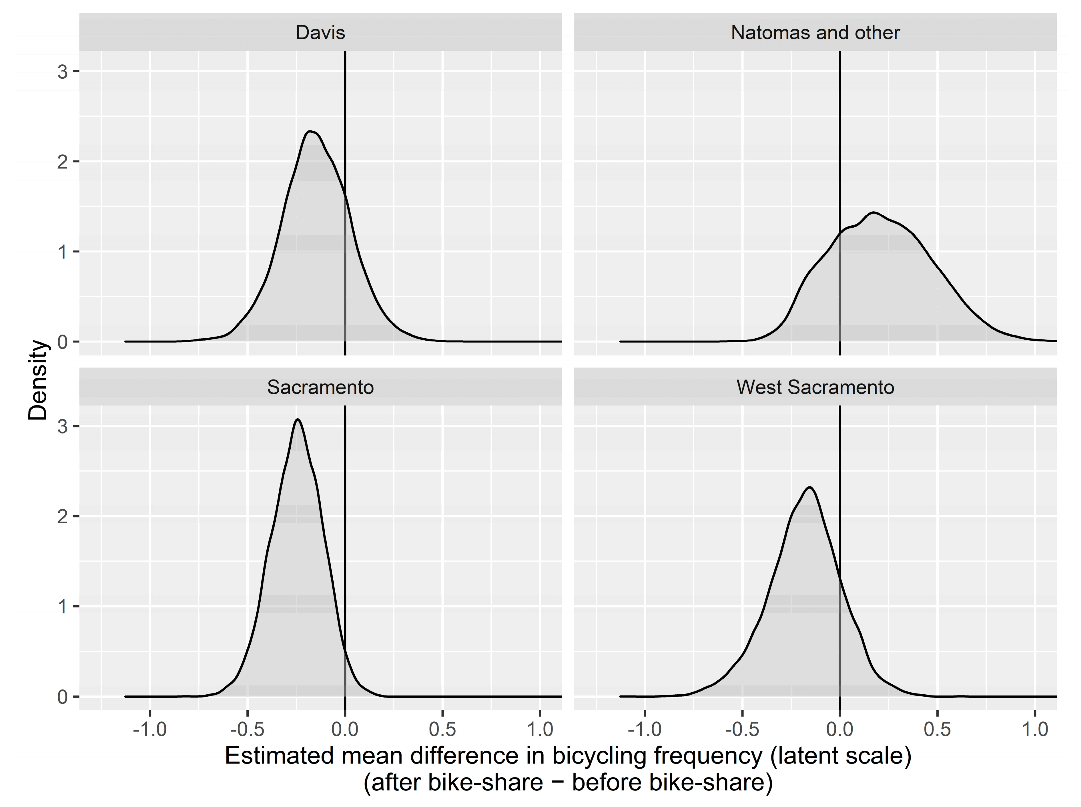
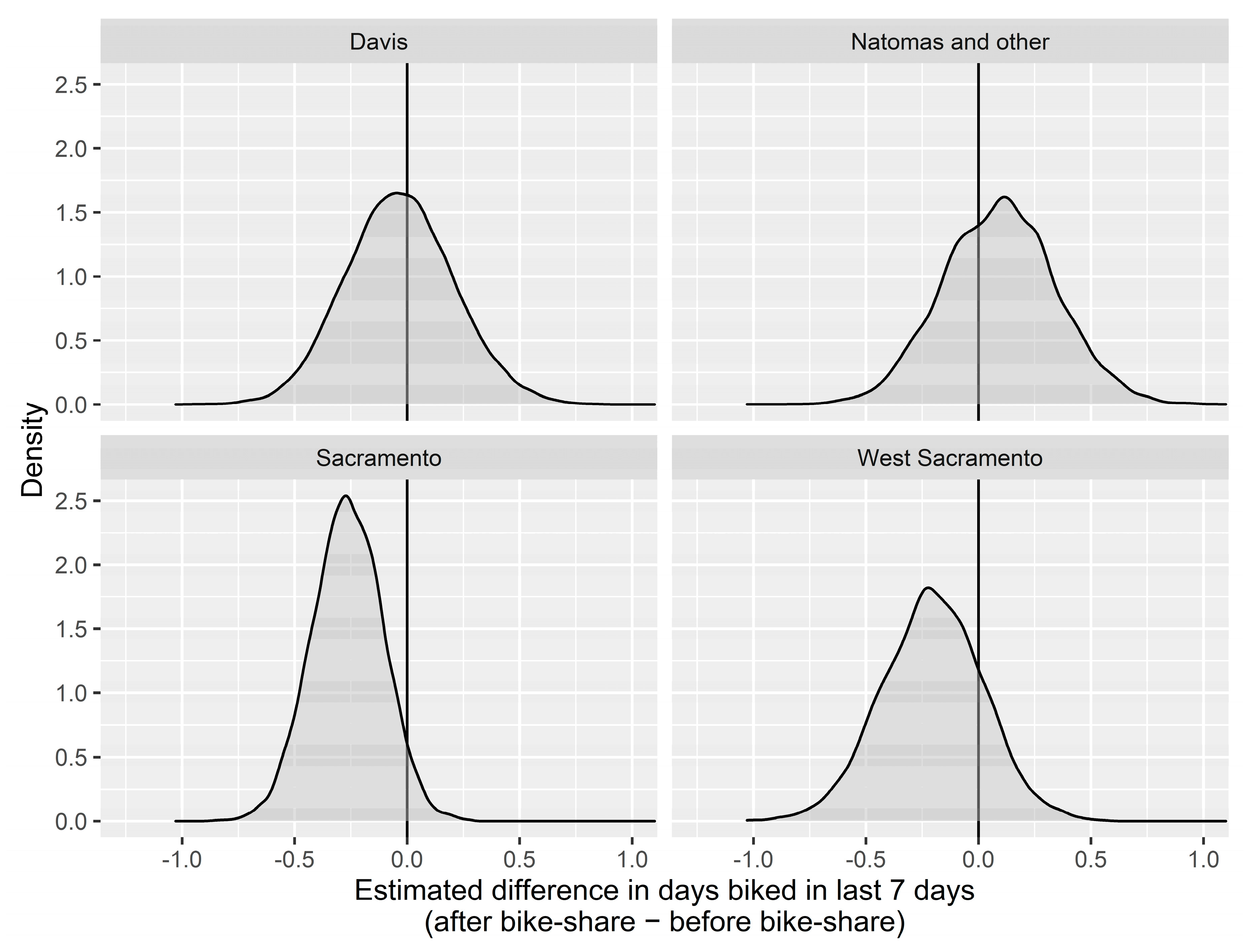
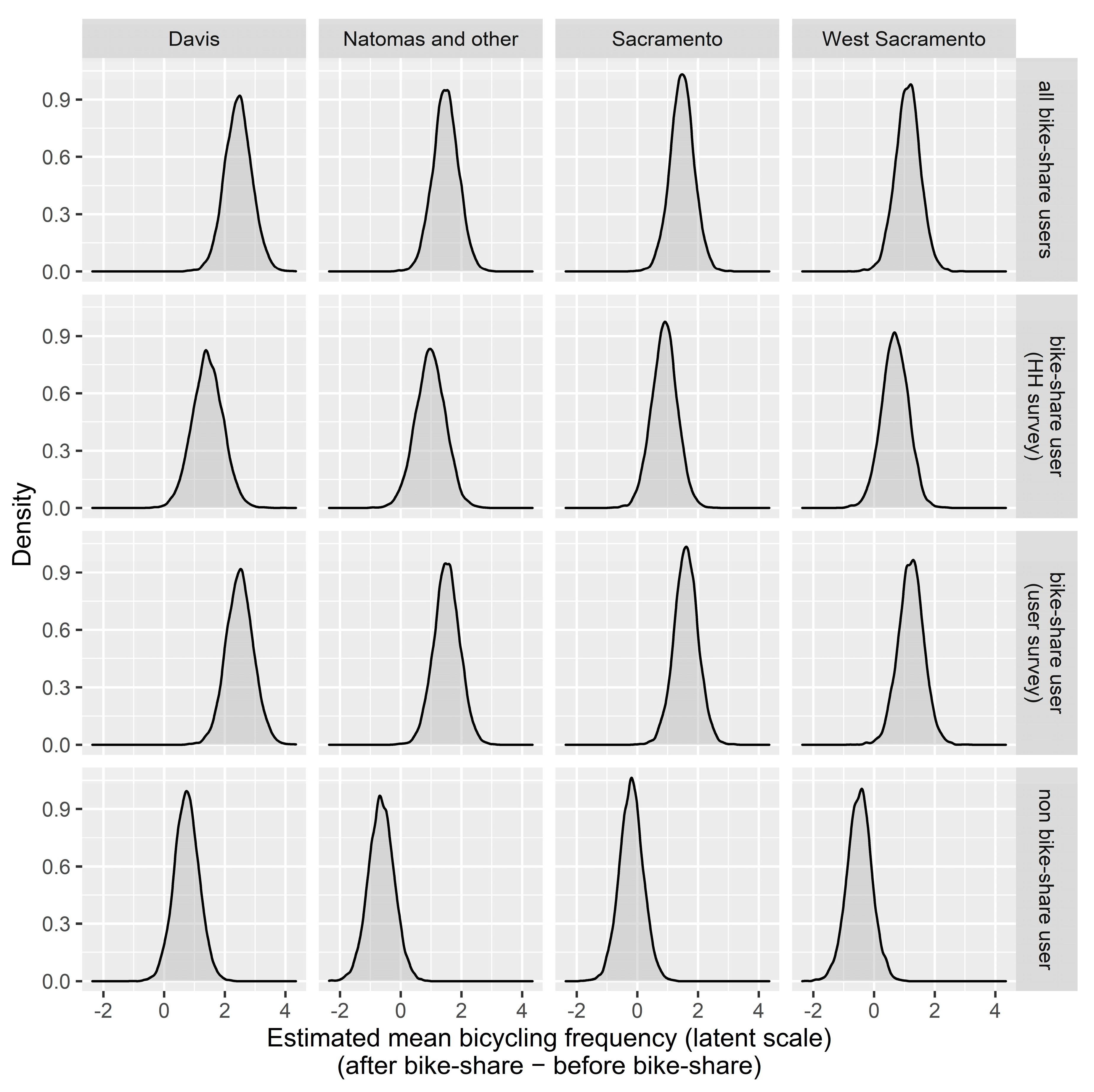
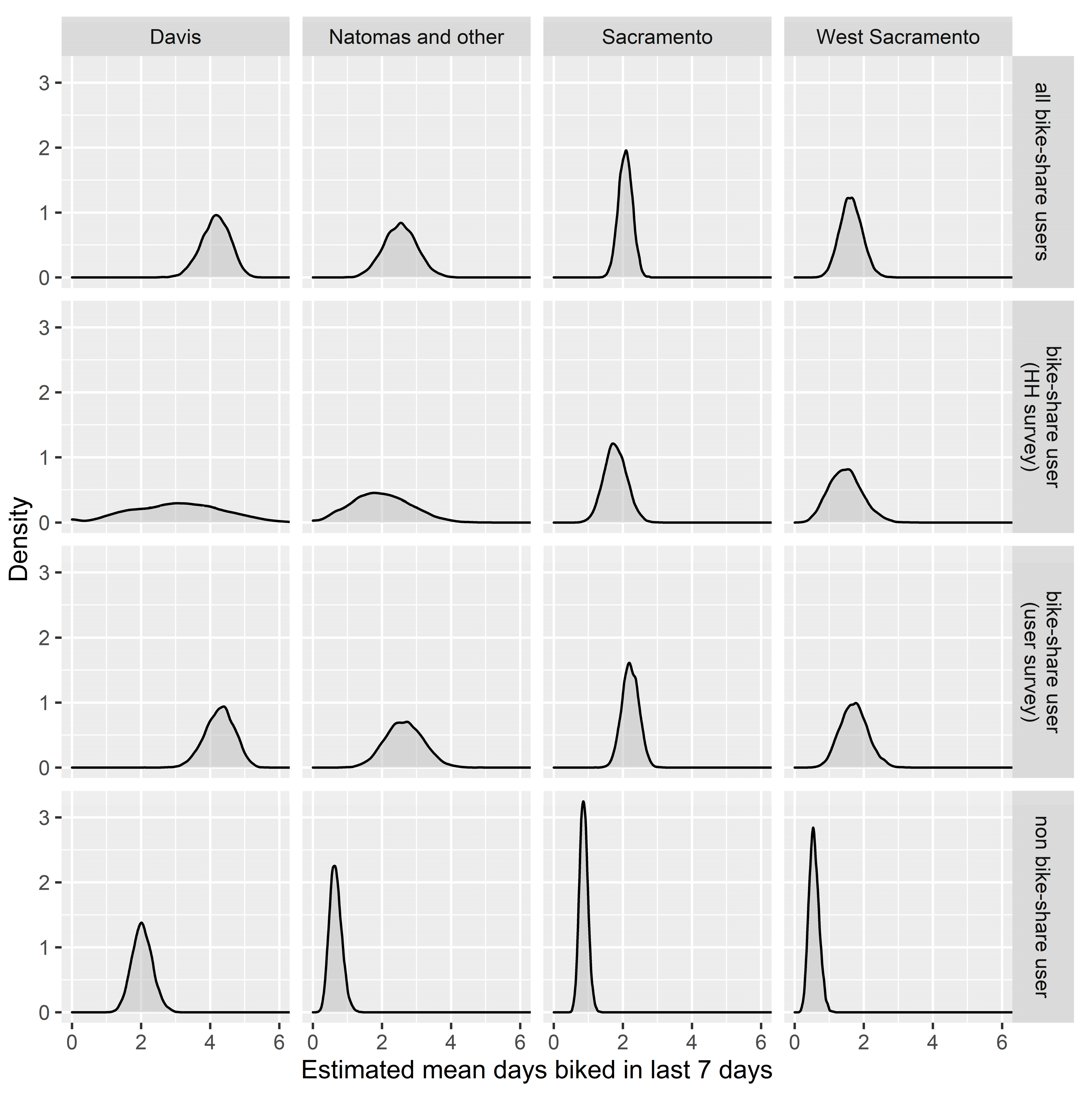
3.2. Bicycling Before-and-After Bike-Share

Summary statistics suggest that several changes may have occurred in bicycling behavior in the three years between the two household surveys. The self-reported number of days bicycled in the last 7 days using either a privately-owned bicycle or the bike-share service dropped from 1.7 days to 1.1 days between 2016 and 2019. However, the household respondents who reported having used the bike-share service rode a bike on 1.9 days on average in 2019, which is 84% greater than the overall average in 2019.

The daily bicycling of all user survey respondents is higher than for the household survey respondents who reported using bike-share: 2.8 days on average in the past 7 days. The greater bicycling rate of the user survey respondents, in comparison to the users from the household survey, suggests their responses likely over-estimate the bicycling of the general population of bike-share users. With that caveat, the distribution of bike-share use according to the user survey is heavily skewed: the median frequency of bike-share use in the past 28 days is 5 trips, the mean is 12.3 trips, and the maximum is 218 trips. The skew in individual-level bike-share frequency indicates that a small group of bike-share users behave very differently than most users. Given the recruitment methods for the two surveys, it is not surprising that we were more likely to capture high frequency users in the user survey than in the household survey.

While these differences in bicycling before-and-after bike-share are notable, they are unadjusted for a variety of factors other than bike-share that could have caused them, and unadjusted for the differences in the before and after samples. Multilevel models that adjust for a series of factors (see Table 2) indicate that differences in bicycling before-and-after bike-share are likely to be small and in many cases the direction of difference is uncertain (see Figure 3 and Figure 4). After bike-share, the frequency of bicycling in general (i.e., not just bike-share) in Davis, Sacramento, and West Sacramento slightly declines (Figure 3), but that decline is not estimated to be greater than 1 day per week on average in any of the cities (Figure 4). The Natomas neighborhood (the sample for which includes user survey respondents living in other neighborhoods outside of the bike-share service area) is the only area where bicycling is not likely to have decreased after bike-share according to the models.

To better understand the effect of bike-share on bicycling, we also use the same models to predict differences by groups of respondents (Figure 5 and Figure 6). The predictions in Figure 5 indicate that people who have used bike-share ride a bike at much greater frequencies than those who have never used bike-share. These differences are similar between the household and user survey respondents, though user survey respondents bicycle at greater frequencies. The adjusted positive association of using bike-share and general bicycling is roughly eight times stronger than the negative before-and-after association between bike-share implementation and population-level bicycling.

These differences in bicycling are also seen in the model predictions of days bicycled in the past 7 days (Figure 6) where bike-share users are predicted to ride a bike approximately twice as many days per week compared to their neighbors who have never used bike-share. Like the effects on general bicycling frequency, using bike-share has a much stronger positive association with days bicycled (Figure 6) than the negative association with bike-share implementation on days bicycled for the general population (Figure 4).

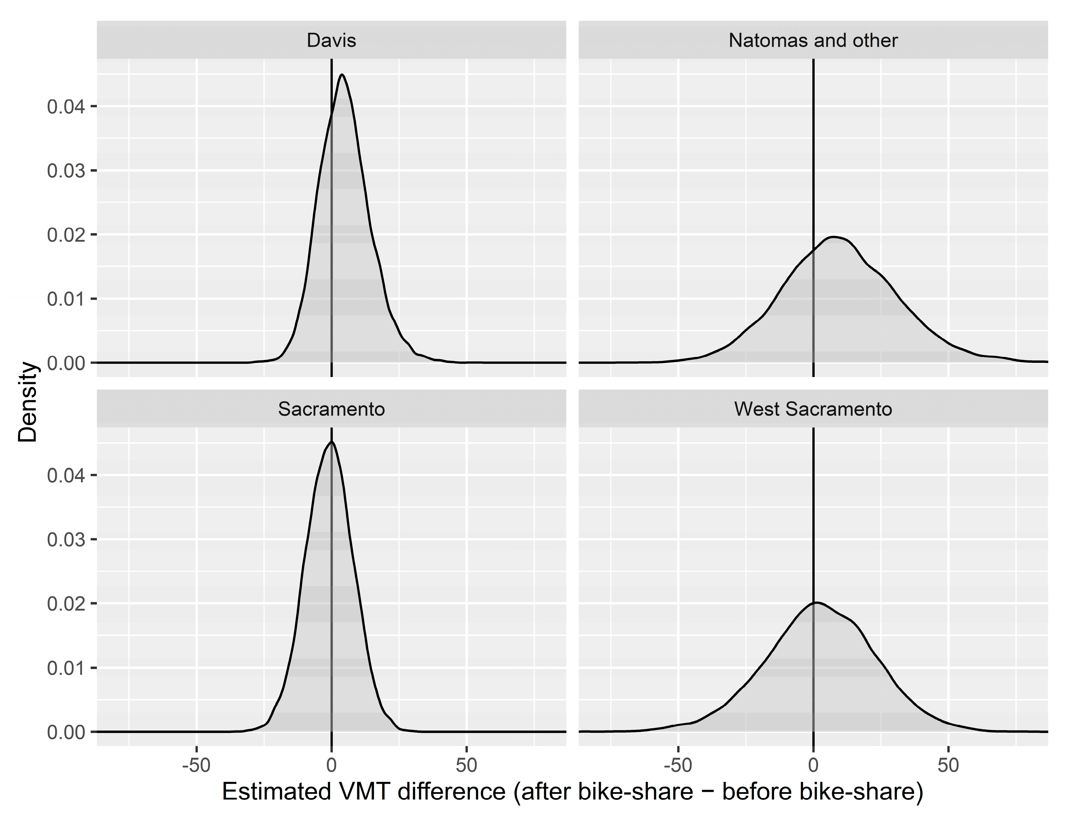
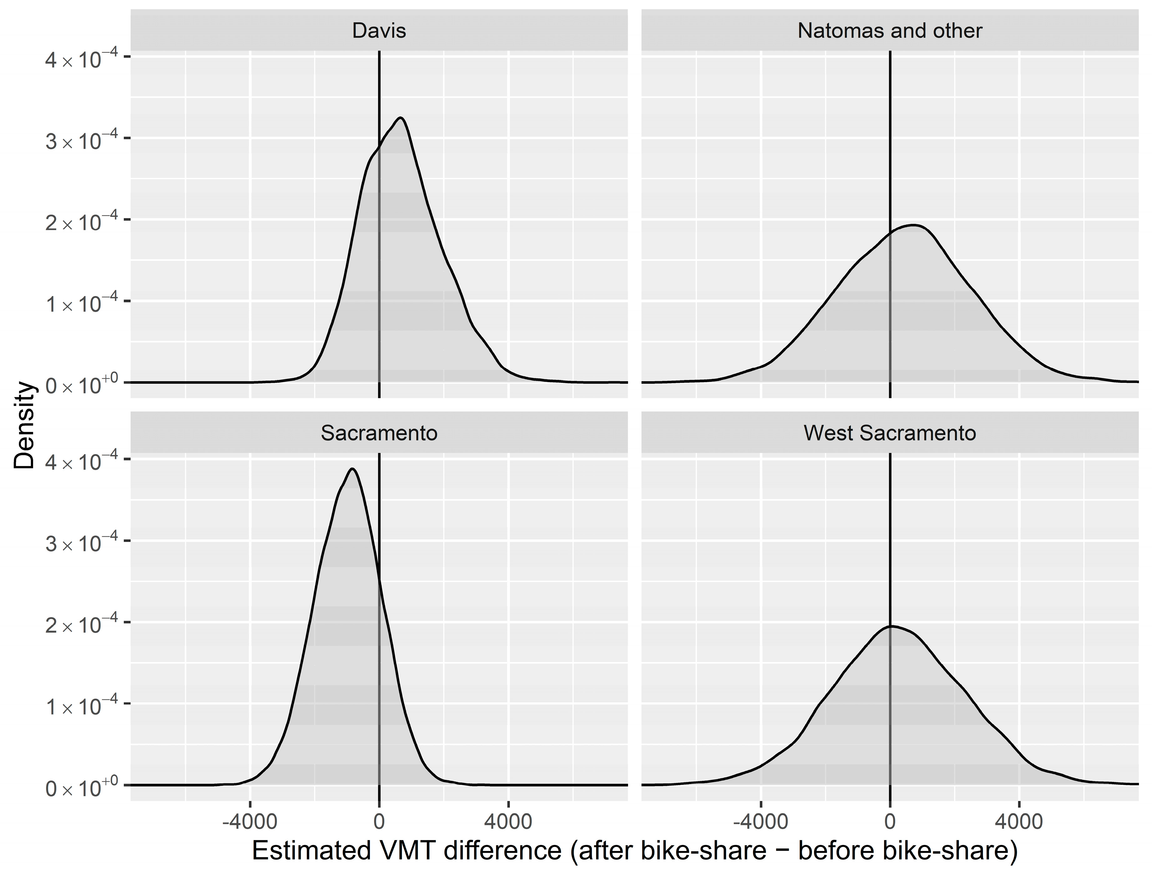
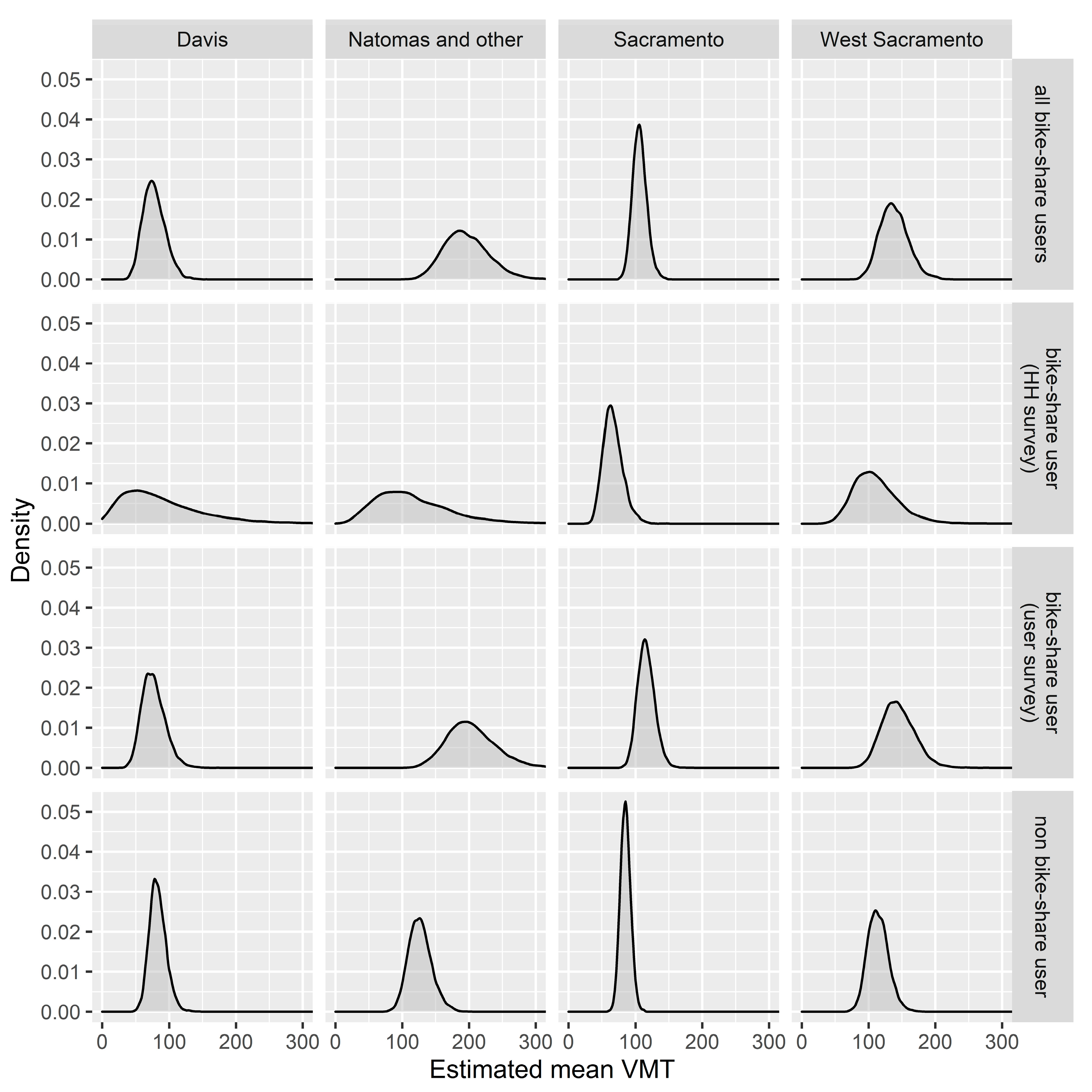
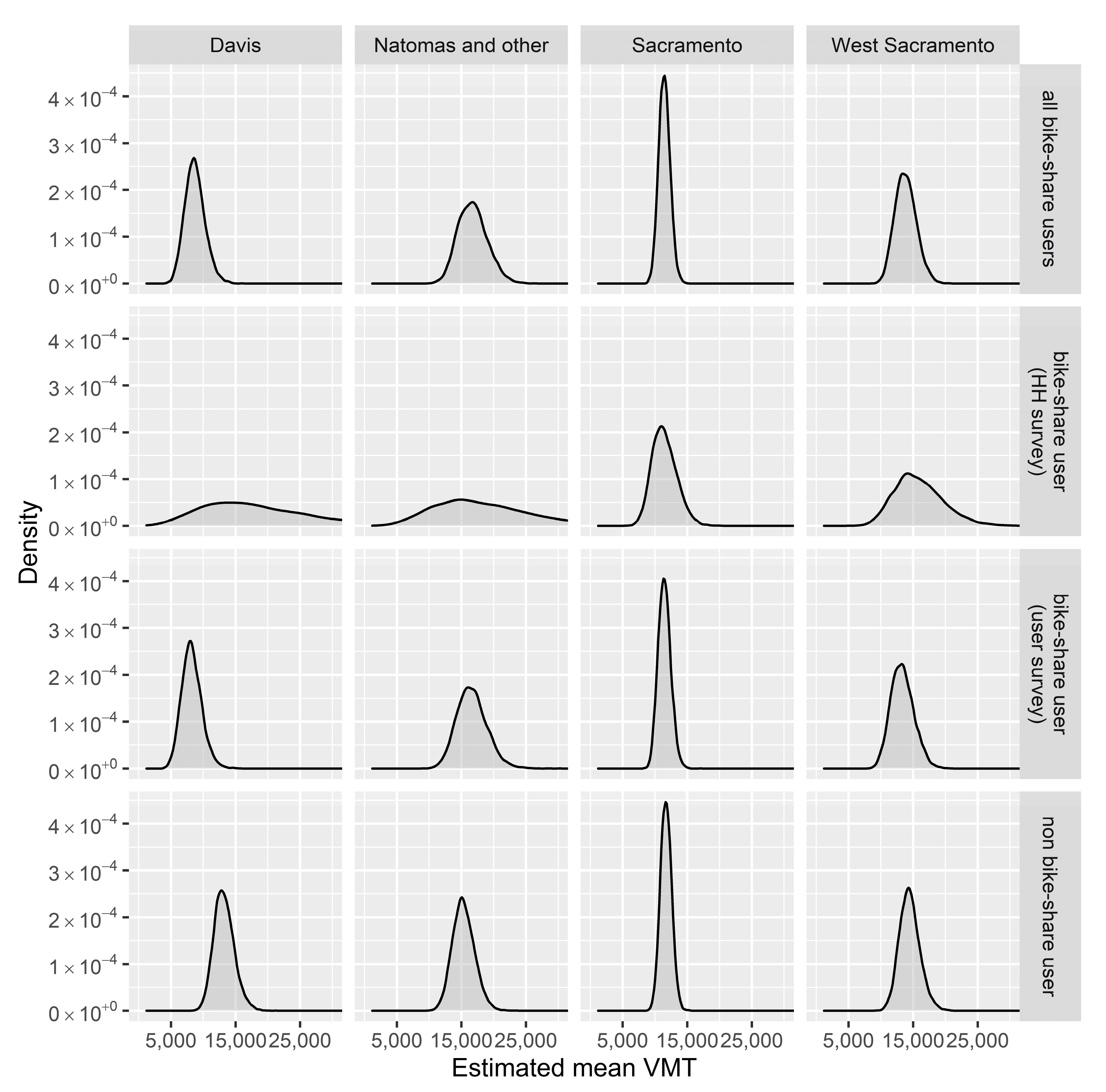
3.3. Driving Before-and-After Bike-Share

After pooling the household and user survey data, simple before-and-after measurements of self-reported personal weekly VMT show an increase (median increased by 10 miles) while annual household VMT shows a decrease (median decreased by 1000 miles). However, inter-person (or household) variation in VMT is large (standard deviations of 121 miles for personal weekly VMT and 10,600 miles for annual household VMT). City level variation in VMT is also large with Davis and Sacramento residents reporting less VMT than residents from West Sacramento and Natomas.

Model predictions of VMT, however, show that on average bike-share had a negligible effect on resident VMT across all neighborhoods (Figure 7 and Figure 8). Residents of Sacramento are the only group with predicted VMT lower after bike-share, but only for annual household VMT (not personal weekly VMT) and it is of a small magnitude (Figure 8). The models similarly predict little difference in respondent weekly VMT and annual household VMT for bike-share users and non-users (Figure 9 and Figure 10). In general, the precision of each prediction reflects the sample size of the group, with large group sizes showing much less uncertainty in mean VMT compared to smaller groups (e.g., household recruited bike-share users).

While our models predict negligible association between bike-share use and annual household VMT, in some cases substantial differences in personal VMT are estimated based on how we sampled users. In all neighborhoods, predicted weekly VMT was greater for intercept-recruited bike-share users, compared to household-recruited bike-share users (Figure 9). In Natomas, the effect of sampling was a doubling of VMT. This suggests that not only were intercept-recruited bike-share users bicycling more frequently (see above), but they were also driving greater distances than household-recruited bike-share users.

4. Discussion

4.1. Bike-Share Adoption

Adoption of bike-share was substantial across the region, particularly given the relatively short time period between the launch of the service and the implementation of the “after” household survey. According to the household survey, 13% of the population in West Sacramento and Sacramento had used the bike-share at least once. On the other hand, only 3% respondents in Davis said they had used bike-share, a surprising result given the high level of bicycling in Davis in general. The low adoption in Davis might be due to the under-sampling of the student population, who are, anecdotally, the most prevalent bike-share users in Davis; only 21% of respondents in the “after” household survey were students, who make up around 36% of the population in Davis based on the 5-year estimates from the American Community Survey. However, none of the UC Davis students who responded in the “after” household survey had used bike-share and only 25% of the Davis respondents to the user survey were students, so it is possible that person-level adoption is, in reality, much lower in Davis, where bike ownership is high and where residents may have seen less need to use bike-share than in the other neighborhoods.

The younger average age of users compared to non-users may be due to numerous factors such as targeted marketing of the service, smartphone technology adoption, or attitudes toward bicycling safety, among others. Bike-share services have historically attracted young users [19]. The high share of students among users outside of Davis may be driven by Sacramento State University and Sacramento City College, both located within the Sacramento service area. For other socio-demographic strata (race, income, etc.), the shares of users and non-users are consistent across groups, though the sample size in some demographic groups is quite small.

Indeed, the surveys underrepresent low-income (< USD 50,000) households, and Black and Hispanic residents (see Table 1). It is telling that we only received a single survey from members of the Boost bike-share subsidy program that provides access to the service for low-income residents (people that are eligible for SMUD Energy Assistance Program, Women, Infants, and Children (WIC), Sacramento Housing and Redevelopment Agency (SHRA), PG&E CARE, and Cal Fresh can participate in the Jump Boost Plan). Nonetheless, a greater percentage of respondents from carless households have used the bike-share service (15% compared to 11% for car households), which may contribute to transportation equity if the lack of car access is a constraint and not a choice. The lack of low income, Black, and Hispanic representation in our surveys suggests that inferences about who is using bike-share may be biased due to survey self-selection.

4.2. The Effects of Bike-Share on Travel Behavior

Bicycling appears to have declined between 2016 and 2019, based on both unadjusted differences (after–before) and on modeled effects of bike-share (Figure 4 and Figure 5). The model predictions indicate that bicycling frequency, measured in two ways, was 5–10% lower after bike-share on average (with a large predicted range). Bicycling rates were mostly stagnant across the country from 2001 to 2017 [20], so it is surprising to find a decline in bicycling in the Sacramento region, particularly since bicycling infrastructure expanded in the region from 2016 to 2019. This bicycling decline warrants further investigation since it is unlikely to have been caused by the emergence of bike-share (see below).

While population-level measures of bicycling may be declining in the Sacramento region, our models predict that people who have used the bike-share service (at least once) bicycle at much greater frequencies than non-users, depending on neighborhood. The model of general bicycling frequency predicts that people who have used the bike-share (at least once) are on average 40–67% more likely to ride nearly every day depending on neighborhood (also see Figure 8 and Figure 9 for a latent variable representation of this difference). The model of days bicycled in the last 7 days predicts a doubling of bicycling days per week for bike-share users relative to non-users. Because little attention has been given to the relationship between bike-share use and general bicycling [7], these predictions offer an important first step for quantifying how much bike-share might increase bicycling. While these results suggest that bike-share may increase bicycling for those who use it, it is also possible that those who bicycle more in general are more likely to use bike-share. Because our data come from repeat cross-sectional surveys rather than a longitudinal survey, we cannot directly assess which direction of causality is stronger, but both are likely to operate to some degree.

Bike-share use could cause individuals to bicycle more in two basic ways. First, an individual’s use of bike-share could directly cause an increase in bicycling if they regularly incorporate the bike-share service into their daily travel routine. Other user survey responses indicated that the median number of bike-share trips per respondent was five trips in 28 days and that 84% of bike-share trips substituted for modes other than bicycling [16]. This result is consistent with other studies that indicate that bike-share rarely replaces personal bike trips [12], and that bike-share users tend to self-report that they increase their bicycling as a result of using bike-share [21]. Five trips in four weeks, with 84% of those trips representing new bicycle trips, is roughly equivalent to an increase in one day of bicycling per week assuming respondents were not otherwise bicycling on that day. Second, bike-share use could spur more personal bicycling. Many causal mechanisms could explain this effect including the visibility of the shared bikes acting as a reminder that bicycling is an option, an increase in perceived safety from seeing people on shared bikes, or possibly through people trying the bike-share service and then in turn shifting to a personal bike. The fact that the bikes in the Sacramento system were e-bikes might also have had an effect, given that awareness of e-bikes increased after the system opened [22]. Because we did not collect data on these potential causes, further research is needed to understand to what degree the model predictions are causally linked from bike-share use to general bicycling, rather than the opposite.

Models of the effect of the bike-share on driving are all fairly inconclusive about the direction and uncertain about the magnitude of any effect bike-share may have had. The predictions suggest that the effect is likely to be small in Sacramento and Davis (less than 25 miles per week) but larger in West Sacramento and Natomas (less than 50 miles per week) (Figure 7). Similarly, annual household VMT may not be associated with bike-share given that our models predict the difference before and after bike-share to be within 4000 miles per year (Figure 8). Only Sacramento residents were predicted to have decreased VMT after bike-share, but the effect is small (1000 miles) and unlikely to have been caused by bike-share given the other results. The Natomas intercept-recruited bike-share users were the only group predicted to have a substantial difference in personal VMT—higher than before bike-share, and higher than the other neighborhoods. This is likely an artifact of the recruitment method for the intercept survey, which resulted in a sample for that combined “after” household and wave 2 user surveys that included a wider range of residential locations (owing to the user surveys) than the sample in the “before” survey, which was limited to the selected neighborhoods (see Figure 2). In general, the lack of a clear relationship between bike-share and driving is not surprising given other studies showing that car substitution is rare [7,12]. However, it is somewhat more surprising in this study because bike-share users self-reported that 35% of their bike share trips substituted for car use (private car and ridehailing) [16].

Given that (a) most bike-share users use bike-share infrequently (median of 5, mean of 12.4 trips in 28 days), (b) bike-share trips are short (mean of 2.1 miles), and (c) about 35% of bike-share trips replace car trips [16], it is unlikely that any predicted differences in VMT from our models are caused by bike-share trips substituting for car trips. Using these mean estimates, we would expect an average bike-share user to reduce their vehicle miles by only 9.1 miles per week as a result of using bike-share. This effect is well within the uncertainty in our models of personal VMT, suggesting that more precise data on VMT is needed to understand any link between bike-share and VMT. In addition, it may be that bike-share has other indirect effects on driving (e.g., attracts people to live in the bike-share service boundary and reduce driving because of increased accessibility), but like the hypothesized indirect effects on bicycling, this is speculative given that we lack data on these causal pathways.

5. Conclusions

Bike-share services have the potential to increase bicycling and decrease driving. However, few studies have attempted to quantify the effects of bike-share services on general bicycling and driving at an individual level. Our results suggest that the dockless e-bike share in the greater Sacramento region is unlikely to have affected average bicycling and driving for residents who live within the bike-share service region. However, our results also suggest that people who have used bike-share ride a bike at substantially greater frequencies: 40–67% more daily bicycling and double the number of days bicycled per week compared to people who have not used bike-share. Because the percent of bike-share trips replacing personal bicycling trips is small, the more frequent bicycling by bike-share users is likely to be at least partially caused by bike-share.

More broadly, our study provides more evidence that bike-share services are increasing bicycling and because of that they still hold potential to help reduce car use. However, demand for these services must grow for them to have lasting impacts on transportation sustainability. Barriers to bike-share adoption are numerous, but limited bike availability and poor bicycling infrastructure are likely the most important barriers that must be removed to increase the contribution of bike-share to transportation sustainability [11]. Additionally, pairing policies that improve bike-share with policies that demote car use (e.g., car free zones, parking pricing) are likely to be more effective at increasing bike-share demand. This combination of policies has worked in some cities to increase general bicycling [23], and recent efforts like those in Paris, France [24] include micromobility services as a key component in the goal to shift from cars to bikes and scooters.

Further investigations into improved operations and bike-share effects on travel behavior more broadly are likely to improve our understanding of what makes for a successful micromobility service. Improved (and more costly) study designs such as longitudinal panels are needed to provide more certainty about the causal effects of micromobility services on travel behavior. Additionally, evaluations of policies and practices are of growing importance as micromobility services become more widespread and as a result more varied. Studies that can identify policies and practices that best increase micromobility demand while at the same time curtailing car use can provide important guidance for ensuring that micromobility services increase transportation sustainability.

Author Contributions

Conceptualization, D.T.F. and S.L.H.; methodology, D.T.F. and S.L.H.; software, D.T.F. and H.M.; validation, D.T.F. and H.M.; formal analysis, D.T.F., S.L.H, and H.M.; investigation, D.T.F., S.L.H, and H.M.; resources, D.T.F. and S.L.H.; data curation, D.T.F. and H.M.; writing—original draft preparation, D.T.F.; writing—review and editing, D.T.F., S.L.H., and H.M.; visualization, D.T.F.; supervision, D.T.F. and S.L.H.; project administration, D.T.F.; funding acquisition, D.T.F. and S.L.H. All authors have read and agreed to the published version of the manuscript.

Funding

This research was funded by California Senate Bill 1.

Institutional Review Board Statement

The study was conducted according to the guidelines of the Declaration of Helsinki, and approved by the Institutional Review Board of the University of California, Davis (protocol code 1325735-1 on 15 October 2018).

Informed Consent Statement

Informed consent was obtained from all subjects involved in the study.

Data Availability Statement

The de-identified portion of the data presented in this study are available on request from the corresponding author. The data are not publicly available due to privacy concerns.

Acknowledgments

The authors would like to thank all the survey respondents, Zhenzi Zhang for managing recruitment and data analysis during this project, and to Yuyou Chen, Zeyu Gao, I-Ju Wang, Salvador Grover, Run Lin Ruan, Kayla Gibson, William Sles, and Belen Garcia for their relentless work to recruit Jump users in the streets. Specific thanks to Sacramento Area Council of Governments and Jump for partnering on this study.

Conflicts of Interest

The authors declare no conflict of interest. The funders had no role in the design of the study; in the collection, analyses, or interpretation of data; in the writing of the manuscript, or in the decision to publish the results.

Appendix A

We modeled four behavioral outcome variables (days bicycled in the last 7 days, usual bicycling frequency, personal weekly VMT, household annual VMT). Each type of response variable required a different model form as outlined below. Although the survey includes before-and-after data, the data do not represent two measurements for each person (i.e., it is not a longitudinal panel). Without panel data, inferences about “change” are heavily dependent on assumptions that the before and after populations are the same. Rather than assume that the samples are the same before and after the bike-share, we chose to “adjust” the effects by considering a suite of covariates in multivariable models. In addition, we merged data from the user survey (targeted recruitment of bike-share users) to increase the sample size of users. Like our adjustments for the other covariates, we include an indicator variable for responses from this non-probability-based recruitment to adjust for any recruitment bias. Overall, the models help represent the effect of the bike-share on each outcome given the uncertainty of the sameness of the two samples. In the statistical models, a multi-level structure is used for each neighborhood area (Davis, West Sacramento, Sacramento, Natomas (Sacramento control)) because of the sampling design. These varying effects help account for the differences in targeted addresses across the four areas before and after the bike-share (e.g., in Davis we over sampled in wave 1 for a concurrent project). We also allowed the effect of the bike-share to vary across these areas by including “varying slopes” for the following binary indicator variables: after bike-share, user survey respondent, respondent had ever used bike share.

For each model parameter, we chose priors by simulating outcome data from our priors alone and ensured that they simulated data in a reasonable range for each outcome. These simulations helped define priors that were “weakly informative” in that they guard against overfitting to the data by using our domain knowledge. For example, when modeling days biked in last 7 days, since we knew from prior surveys that most people do not bicycle at all, we set priors that simulated data such that it was rare for the model to predict a negligible portion “zero” counts, while at the same time making it rare to predict all of the responses to be “zero” counts. In another example, for the VMT data, we knew it was rare for weekly VMT to be more than a few thousand miles, so we settled on priors that ensured this. Our general process for selecting priors was as follows: (1) use the default prior the R package brms [18], (2) plot simulated data as histograms for 30 datasets, (3) adjust the priors and re-plot the histograms to ensure the simulations result in a reasonable range for each outcome (allowing a few extremes but not always resulting in extremes). Repeat steps 2 and 3 as needed. Below are the general model forms for each analysis including their priors.

Days biked in last 7 days
$y_{i}$	$~ Zero - Inflated Binomial (7, p_{i}, k_{i})$
$logit (p_{i})$	$= α_{p} + α_{p_c i t y [i]} + β_{p A_c i t y [i]} A_{i} + β_{p S_c i t y [i]} S_{i} + β_{p U_c i t y [i]} U_{i} + \sum_{m = 1}^{M} β_{p m} X_{m i}$
$logit (k_{i})$	$= α_{k} + α_{k_c i t y [i]} + β_{k A_c i t y [i]} A_{i} + β_{k S_c i t y [i]} S_{i} + β_{k U_c i t y [i]} U_{i} + \sum_{m = 1}^{M} β_{k m} X_{m i}$
$[\begin{matrix} \begin{matrix} α_{p_c i t y} \\ β_{p A_c i t y} \\ β_{p S_c i t y} \end{matrix} \\ β_{p U_c i t y} \end{matrix}]$	$~ MVNormal ([\begin{matrix} \begin{matrix} 0 \\ 0 \end{matrix} \\ 0 \\ 0 \end{matrix}], Σ_{p})$
$[\begin{matrix} \begin{matrix} α_{k_c i t y} \\ β_{k A_c i t y} \\ β_{k S_c i t y} \end{matrix} \\ β_{k U_c i t y} \end{matrix}]$	$~ MVNormal ([\begin{matrix} \begin{matrix} 0 \\ 0 \end{matrix} \\ 0 \\ 0 \end{matrix}], Σ_{k})$
$Σ_{p}$	$= (\begin{matrix} σ_{p_α} & 0 & 0 \\ 0 & ⋱ & 0 \\ 0 & 0 & σ_{p_β_{U}} \end{matrix}) Ω_{p} (\begin{matrix} σ_{p_α} & 0 & 0 \\ 0 & ⋱ & 0 \\ 0 & 0 & σ_{p_β_{U}} \end{matrix})$
$Σ_{k}$	$= (\begin{matrix} σ_{k_α} & 0 & 0 \\ 0 & ⋱ & 0 \\ 0 & 0 & σ_{k_β_{U}} \end{matrix}) Ω_{k} (\begin{matrix} σ_{k_α} & 0 & 0 \\ 0 & ⋱ & 0 \\ 0 & 0 & σ_{k_β_{U}} \end{matrix})$
Priors
$(α_{p}, α_{k})$	$~ Normal (0, 1.5)$
$(β_{p 1}, \dots, β_{p m}, β_{k 1}, \dots, β_{k m})$	$~ Normal (0, 0.5)$
$(σ_{p_α}, \dots, σ_{{p_{β}}_{U}}, σ_{k_α}, \dots, σ_{k_β_{U}})$	$~ HalfStudentT (3, 0, 0.5)$
$(Ω_{p}, Ω_{k})$	$~ LKJcorr (2)$

where

y_{i}

is the response from 0 to 7 days for respondent i,

p_{i}

is the linear model for the probability of bicycling each day out of 7 days, and

k_{i}

is the linear model for the probability of not bicycling at all (zero inflation).

α_{p}

and

α_{k}

are the intercepts,

α_{p_c i t y [i]}

and

α_{k_c i t y [i]}

are vectors of intercepts that vary by city,

β_{p A_c i t y [i]}

and

β_{k A_c i t y [i]}

are vectors of slope parameters for the effect of

A_{i}

(a vector of zeros and ones indicating “after bike-share”) that vary by city,

β_{p S_c i t y [i]}

and

β_{k S_c i t y [i]}

are vectors of slope parameters for the effect of

S_{i}

(a vector of zeros and ones indicating sub-sample recruited non-probabilistically in the user survey) that vary by city,

β_{p U_c i t y [i]}

and

β_{k U_c i t y [i]}

are vectors of slope parameters for the effect of

U_{i}

(a vector of zeros and ones indicating having used bike-share) that vary by city,

β_{p m}

and

β_{k m}

are the slopes for their products of

X_{m i}

(predictor variables, m),

Σ_{p}

and

Σ_{k}

are the covariance matrices factored as diagonal matrices of city level standard deviations (

σ_{p_α}, \dots, σ_{{p_{β}}_{U}}, σ_{k_{α}}, \dots, σ_{k_β_{U}}

) and correlation matrices (

Ω_{p}

,

Ω_{k}

) for the aggregate binomial (p) and zero-inflated Bernoulli (k) processes, respectively. Each correlation matrix has six parameters representing the correlations between the four city-varying parameters. This equation is slightly generalized from the actual model because the R package brms automatically parameterizes models (for efficiency reasons) by centering all variables and converting the correlation matrices to Cholesky factors prior to estimation [18].

Bicycling Frequency as ordered categories:	{Never, Not used in the last year, A few times per year, A few timers per month, A few times per week, Every day or almost every day}
$l o g (\frac{P r (y_{i} < k)}{1 - P r (y_{i} < k)})$	$= α_{k} + α_{c i t y [i]} - β_{A_c i t y [i]} A_{i} - β_{S_c i t y [i]} S_{i} - β_{U_c i t y [i]} U_{i} - \sum_{m = 1}^{M} β_{m} X_{m i}$
$[\begin{matrix} \begin{matrix} α_{c i t y} \\ β_{A_c i t y} \\ β_{S_c i t y} \end{matrix} \\ β_{U_c i t y} \end{matrix}]$	$~ M V N o r m a l ([\begin{matrix} \begin{matrix} 0 \\ 0 \end{matrix} \\ 0 \\ 0 \end{matrix}], Σ)$
$Σ$	$= (\begin{matrix} σ_{α} & 0 & 0 \\ 0 & ⋱ & 0 \\ 0 & 0 & σ_{β_{U}} \end{matrix}) Ω (\begin{matrix} σ_{α} & 0 & 0 \\ 0 & ⋱ & 0 \\ 0 & 0 & σ_{β_{U}} \end{matrix})$
Priors
$(α_{1}, \dots, α_{k})$	$~ N o r m a l (0, 1.5)$
$(β_{1}, \dots, β_{m})$	$~ N o r m a l (0, 0.5)$
$(σ_{α}, \dots, σ_{β_{U}})$	$~ H a l f S t u d e n t T (3, 0, 0.5)$
$Ω$	$~ L K J c o r r (2)$

where

\log (\frac{\Pr (y_{i} \leq k)}{1 - \Pr (y_{i} \leq k)})

is the log-cumulative-odds that response value

y_{i}

is equal to or less than a possible response category k (Never, …, Every day or almost every day).

α_{k}

are the threshold intercepts for the k thresholds between the k + 1 response categories.

α_{c i t y [i]}

is the vector of intercepts that vary by city,

β_{A_c i t y [i]}

are vectors of slope parameters for the effect of

A_{i}

(a vector of zeros and ones indicating “after bike-share”) that vary by city,

β_{S_c i t y [i]}

are vectors of slope parameters for the effect of

S_{i}

(a vector of zeros and ones indicating sub-sample recruited non-probabilistically in the user survey) that vary by city,

β_{U_c i t y [i]}

are vectors of slope parameters for the effect of

U_{i}

(a vector of zeros and ones indicating having used bike-share) that vary by city.

β_{m}

are the slopes for their products of

X_{m i}

(predictor variables, m),

Σ

is the covariance matrix factored as a diagonal matrix of city level standard deviations (

σ_{α}, \dots, σ_{β_{U}}

) and correlation matrix

Ω

. The correlation matrix has six parameters representing the correlations between the four city-varying parameters. Each

β_{m} X_{m i}

term is subtracted from the intercepts to ensure a positive

β_{m}

value indicating that an increase in

X_{m i}

results in an increase in the average response. This is because a decrease (hence subtraction) in the log-cumulative-odds for every outcome below the maximum results in a shift of probability toward the higher response categories.

Weekly personal VMT and annual household VMT
$y_{i}$	$~ Hurdle gamma (p_{i}, θ_{i}, k)$
$l o g i t (p_{i})$	$= α_{p} + α_{p_c i t y [i]} + β_{p A_c i t y [i]} A_{i} + β_{p S_c i t y [i]} S_{i} + β_{p U_c i t y [i]} U_{i} + \sum_{m = 1}^{M} β_{p m} X_{m i}$
$l o g (θ_{i})$	$= α_{θ} + α_{θ_c i t y [i]} + β_{θ A_c i t y [i]} A_{i} + β_{θ S_c i t y [i]} S_{i} + β_{θ U_c i t y [i]} U_{i} + \sum_{m = 1}^{M} β_{θ m} X_{m i}$
$[\begin{matrix} \begin{matrix} α_{p_c i t y} \\ β_{p A_c i t y} \\ β_{p S_c i t y} \end{matrix} \\ β_{p U_c i t y} \end{matrix}]$	$~ M V N o r m a l ([\begin{matrix} \begin{matrix} 0 \\ 0 \end{matrix} \\ 0 \\ 0 \end{matrix}], Σ_{p})$
$[\begin{matrix} \begin{matrix} α_{θ_c i t y} \\ β_{θ A_c i t y} \\ β_{θ S_c i t y} \end{matrix} \\ β_{θ U_c i t y} \end{matrix}]$	$~ M V N o r m a l ([\begin{matrix} \begin{matrix} 0 \\ 0 \end{matrix} \\ 0 \\ 0 \end{matrix}], Σ_{θ})$
$Σ_{p}$	$= (\begin{matrix} σ_{p_α} & 0 & 0 \\ 0 & ⋱ & 0 \\ 0 & 0 & σ_{p_β_{U}} \end{matrix}) Ω_{p} (\begin{matrix} σ_{p_α} & 0 & 0 \\ 0 & ⋱ & 0 \\ 0 & 0 & σ_{p_β_{U}} \end{matrix})$
$Σ_{θ}$	$= (\begin{matrix} σ_{θ_α} & 0 & 0 \\ 0 & ⋱ & 0 \\ 0 & 0 & σ_{θ_β_{U}} \end{matrix}) Ω_{θ} (\begin{matrix} σ_{θ_α} & 0 & 0 \\ 0 & ⋱ & 0 \\ 0 & 0 & σ_{θ_β_{U}} \end{matrix})$
Priors
$α_{p}$	$~ Normal (- 3, 1)$
$α_{θ}$	$~ Normal (\log ({\bar{y}}_{i}), 0.7)$
$(β_{p 1}, \dots, β_{p m}, β_{θ 1}, \dots, β_{θ m})$	$~ Normal (0, 0.5)$
$(σ_{p_α}, \dots, σ_{{p_{β}}_{U}}, σ_{θ_{α}}, \dots, σ_{θ_β_{U}})$	$~ Normal (0, 1)$
$(Ω_{p}, Ω_{θ})$	$~ LKJcorr (2)$
$k$	$~ HalfStudentT (5, 0, 2)$

where

y_{i}

is the vehicle miles traveled (including zeros) for respondent i,

p_{i}

is linear model for the probability of zero vehicle miles traveled (hurdle), and

θ_{i}

is the linear model for vehicle miles traveled.

α_{p}

and

α_{θ}

are the intercepts,

α_{p_c i t y [i]}

and

α_{θ_c i t y [i]}

are vectors of intercepts that vary by city,

β_{p A_c i t y [i]}

and

β_{θ A_c i t y [i]}

are vectors of slope parameters for the effect of

A_{i}

(a vector of zeros and ones indicating “after bike-share”) that vary by city,

β_{p S_c i t y [i]}

and

β_{θ S_c i t y [i]}

are vectors of slope parameters for the effect of

S_{i}

(a vector of zeros and ones indicating sub-sample recruited non-probabilistically in the user survey) that vary by city,

β_{p U_c i t y [i]}

and

β_{θ U_c i t y [i]}

are vectors of slope parameters for the effect of

U_{i}

(a vector of zeros and ones indicating having used bike-share) that vary by city,

β_{p m}

and

β_{θ m}

are the slopes for their products of

X_{m i}

(predictor variables, m),

Σ_{p}

and

Σ_{θ}

are the covariance matrices factored as diagonal matrices of city level standard deviations (

σ_{p_α}, \dots, σ_{{p_{β}}_{U}}, σ_{θ_{α}}, \dots, σ_{θ_β_{U}}

) and correlation matrices (

Ω_{p}

,

Ω_{θ}

) for the Bernoulli (p) (hurdle) and gamma (

θ

) processes, respectively. Each correlation matrix has six parameters representing the correlations between the four city-varying parameters. Like the zero-inflated binomial model, this equation is slightly generalized from the actual model parameterization used the R package brms [18].

Appendix B. Model Parameter Summaries

Table A1. Multi-level zero-inflated binomial model of bicycling days in last 7 days parameter summaries.

Parameter Description	Parameter	Mean	sd
Count Binomial Model	$p_{i}$
Intercept	$α_{p}$	0.598	0.257
After bike-share (0/1)	$β_{p 1}$	−0.052	0.164
User survey (0/1)	$β_{p 2}$	0.021	0.228
Ever used bike-share (0/1)	$β_{p 3}$	0.286	0.193
Age (z-score)	$β_{p 4}$	−0.008	0.043
Woman (0/1)	$β_{p 5}$	−0.352	0.055
One Adult HH (0/1)	$β_{p 6}$	−0.220	0.071
No children HH (0/1)	$β_{p 7}$	0.051	0.061
Two or more HH cars (0/1)	$β_{p 8}$	−0.431	0.063
No College Degree (0/1)	$β_{p 9}$	−0.100	0.096
Working (0/1)	$β_{p 10}$	−0.099	0.070
Student (0/1)	$β_{p 11}$	0.141	0.134
>USD 50,000 HH income (0/1)	$β_{p 12}$	−0.291	0.110
Physical condition, cannot ride bike (0/1)	$β_{p 13}$	−0.532	0.140
Student × >USD 50,000 HH income (0/1)	$β_{p 14}$	0.132	0.157
Zero-Inflated Bernoulli Model	$k_{i}$
Intercept	$α_{k}$	0.591	0.461
After bike-share (0/1)	$β_{k 1}$	0.107	0.225
User survey (0/1)	$β_{k 2}$	−0.297	0.294
Ever used bike-share (0/1)	$β_{k 3}$	−0.908	0.298
Age (z-score)	$β_{k 4}$	0.125	0.066
Woman (0/1)	$β_{k 5}$	0.486	0.096
One Adult HH (0/1)	$β_{k 6}$	0.439	0.127
No children HH (0/1)	$β_{k 7}$	0.178	0.111
Two or more HH cars (0/1)	$β_{k 8}$	0.062	0.116
No College Degree (0/1)	$β_{k 9}$	−0.279	0.164
Working (0/1)	$β_{k 10}$	−0.248	0.125
Student (0/1)	$β_{k 11}$	−0.818	0.212
>USD 50,000 HH income (0/1)	$β_{k 12}$	−0.227	0.165
Physical condition, cannot ride bike (0/1)	$β_{k 13}$	0.941	0.186
Student × >USD 50,000 HH income (0/1)	$β_{k 14}$	0.430	0.258
Neighborhood Level Variation
Count Binomial Model
Std. dev. Intercept	$σ_{p_α}$	0.383	0.196
Std. dev. Ever used bike-share	$σ_{p_β_{A}}$	0.240	0.208
Std. dev. User survey	$σ_{p_β_{S}}$	0.372	0.256
Std. dev. After bike-share	$σ_{p_β_{U}}$	0.267	0.194
Zero-Inflated Bernoulli Model
Std. dev. Intercept	$σ_{k_α}$	0.759	0.321
Std. dev. Ever used bike-share	$σ_{k_β_{A}}$	0.340	0.324
Std. dev. User survey	$σ_{k_β_{S}}$	0.309	0.273
Std. dev. After bike-share	$σ_{k_β_{U}}$	0.392	0.242
Varying parameter correlations by neighborhood
Count Binomial Model
Cor. Intercept and Ever used bike-share	$Ω_{p 1}$	0.044	0.380
Cor. Intercept and User survey	$Ω_{p 2}$	−0.131	0.355
Cor. Ever used bike-share and User survey	$Ω_{p 3}$	−0.061	0.379
Cor. Intercept and After bike-share	$Ω_{p 4}$	0.169	0.354
Cor. Ever used bike-share and After bike-share	$Ω_{p 5}$	−0.028	0.372
Cor. User survey and After bike-share	$Ω_{p 6}$	−0.109	0.367
Zero-Inflated Bernoulli Model
Cor. Intercept and Ever used bike-share	$Ω_{k 1}$	−0.038	0.376
Cor. Intercept and User survey	$Ω_{k 2}$	0.082	0.378
Cor. Ever used bike-share and User survey	$Ω_{k 3}$	−0.044	0.384
Cor. Intercept and After bike-share	$Ω_{k 4}$	−0.186	0.343
Cor. Ever used bike-share and After bike-share	$Ω_{k 5}$	0.030	0.374
Cor. User survey and After bike-share	$Ω_{k 6}$	−0.022	0.374

Table A2. Multi-level ordered logit model of general bicycling frequency parameter summaries.

Parameter Description	Parameter	Mean	sd
Intercept [1]	$α_{1}$	−1.575	0.384
Intercept [2]	$α_{2}$	−0.659	0.383
Intercept [3]	$α_{3}$	0.150	0.383
Intercept [4]	$α_{4}$	1.061	0.383
Intercept [5]	$α_{5}$	2.207	0.385
After bike-share (0/1)	$β_{1}$	−0.086	0.197
User survey (0/1)	$β_{2}$	0.469	0.236
Ever used bike-share (0/1)	$β_{3}$	0.884	0.247
Age (z-score)	$β_{4}$	−0.140	0.053
Woman (0/1)	$β_{5}$	−0.537	0.075
One Adult HH (0/1)	$β_{6}$	−0.254	0.102
No children HH (0/1)	$β_{7}$	−0.173	0.085
Two or more HH cars (0/1)	$β_{8}$	−0.153	0.093
No College Degree (0/1)	$β_{9}$	0.084	0.134
Working (0/1)	$β_{10}$	0.343	0.099
Student (0/1)	$β_{11}$	0.916	0.187
>USD 50,000 HH income (0/1)	$β_{12}$	0.251	0.141
Physical condition, cannot ride bike (0/1)	$β_{13}$	−1.076	0.169
Student × >USD 50,000 HH income (0/1)	$β_{14}$	−0.560	0.217
Neighborhood Level Variation
Std. dev. Intercept	$σ_{α}$	0.738	0.283
Std. dev. Ever used bike-share	$σ_{β_{A}}$	0.283	0.254
Std. dev. User survey	$σ_{β_{S}}$	0.266	0.223
Std. dev. After bike-share	$σ_{β_{U}}$	0.325	0.219
Varying Parameter Correlations by Neighborhood
Cor. Intercept and Ever used bike-share	$Ω_{1}$	−0.153	0.368
Cor. Intercept and User survey	$Ω_{2}$	−0.140	0.368
Cor. Ever used bike-share and User survey	$Ω_{3}$	−0.015	0.373
Cor. Intercept and After bike-share	$Ω_{4}$	−0.165	0.342
Cor. Ever used bike-share and After bike-share	$Ω_{5}$	0.034	0.371
Cor. User survey and After bike-share	$Ω_{6}$	0.023	0.377

Table A3. Multi-level hurdle-gamma model of respondent weekly VMT parameter summaries.

Parameter Description	Parameter	Mean	sd
Zero-VMT Binary Model (Hurdle)	$p_{i}$
Intercept	$α_{p}$	−0.082	0.420
After bike-share (0/1)	$β_{p 1}$	−0.074	0.333
User survey (0/1)	$β_{p 2}$	−0.058	0.456
Ever used bike-share (0/1)	$β_{p 3}$	0.369	0.462
Age (z-score)	$β_{p 4}$	−0.234	0.105
Woman (0/1)	$β_{p 5}$	−0.223	0.150
One Adult HH (0/1)	$β_{p 6}$	−0.503	0.184
No children HH (0/1)	$β_{p 7}$	0.514	0.208
Two or more HH cars (0/1)	$β_{p 8}$	−1.564	0.190
No College Degree (0/1)	$β_{p 9}$	−0.806	0.205
Working (0/1)	$β_{p 10}$	−0.498	0.186
Student (0/1)	$β_{p 11}$	−0.179	0.277
>USD 50,000 HH income (0/1)	$β_{p 12}$	−1.174	0.214
Student × >USD 50,000 HH income (0/1)	$β_{p 13}$	0.370	0.347
Greater Than Zero-VMT Gamma Model	$θ_{i}$
Intercept	$α_{θ}$	4.185	0.203
After bike-share (0/1)	$β_{θ 1}$	0.031	0.117
User survey (0/1)	$β_{θ 2}$	0.466	0.215
Ever used bike-share (0/1)	$β_{θ 3}$	−0.208	0.198
Age (z-score)	$β_{θ 4}$	−0.016	0.030
Woman (0/1)	$β_{θ 5}$	−0.152	0.043
One Adult HH (0/1)	$β_{θ 6}$	0.330	0.061
No children HH (0/1)	$β_{θ 7}$	−0.100	0.048
Two or more HH cars (0/1)	$β_{θ 8}$	0.372	0.057
No College Degree (0/1)	$β_{θ 9}$	−0.030	0.086
Working (0/1)	$β_{θ 10}$	0.246	0.061
Student (0/1)	$β_{θ 11}$	−0.217	0.129
>USD 50,000 HH income (0/1)	$β_{θ 12}$	0.140	0.090
Student × >USD 50,000 HH income (0/1)	$β_{θ 13}$	0.026	0.151
Neighborhood Level Variation
Zero-VMT Binary Model (Hurdle)
Std. dev. Intercept	$σ_{p_α}$	0.423	0.311
Std. dev. Ever used bike-share	$σ_{p_β_{A}}$	0.433	0.365
Std. dev. User survey	$σ_{p_β_{S}}$	0.394	0.344
Std. dev. After bike-share	$σ_{p_β_{U}}$	0.439	0.356
Greater Than Zero-VMT Gamma Model
Std. dev. Intercept	$σ_{θ_α}$	0.271	0.193
Std. dev. Ever used bike-share	$σ_{θ_β_{A}}$	0.219	0.224
Std. dev. User survey	$σ_{θ_β_{S}}$	0.253	0.231
Std. dev. After bike-share	$σ_{θ_β_{U}}$	0.147	0.160
Varying parameter correlations by neighborhood
Zero-VMT Binary Model (Hurdle)
Cor. Intercept and Ever used bike-share	$Ω_{p 1}$	0.021	0.384
Cor. Intercept and User survey	$Ω_{p 2}$	−0.013	0.388
Cor. Ever used bike-share and User survey	$Ω_{p 3}$	−0.068	0.386
Cor. Intercept and After bike-share	$Ω_{p 4}$	0.008	0.380
Cor. Ever used bike-share and After bike-share	$Ω_{p 5}$	0.006	0.380
Cor. User survey and After bike-share	$Ω_{p 6}$	−0.031	0.383
Greater Than Zero-VMT Gamma Model
Cor. Intercept and Ever used bike-share	$Ω_{θ 1}$	0.056	0.377
Cor. Intercept and User survey	$Ω_{θ 2}$	−0.055	0.381
Cor. Ever used bike-share and User survey	$Ω_{θ 3}$	−0.068	0.386
Cor. Intercept and After bike-share	$Ω_{θ 4}$	0.026	0.372
Cor. Ever used bike-share and After bike-share	$Ω_{θ 5}$	−0.018	0.378
Cor. User survey and After bike-share	$Ω_{θ 6}$	−0.024	0.382

Table A4. Multi-level hurdle-gamma model of annual household VMT parameter summaries.

Parameter Description	Parameter	Mean	sd
Zero-VMT Binary Model (Hurdle)	$p_{i}$
Intercept	$α_{p}$	−0.910	0.439
After bike-share (0/1)	$β_{p 1}$	0.031	0.322
User survey (0/1)	$β_{p 2}$	0.384	0.537
Ever used bike-share (0/1)	$β_{p 3}$	0.741	0.533
Age (z-score)	$β_{p 4}$	−0.141	0.126
Woman (0/1)	$β_{p 5}$	−0.115	0.184
One Adult HH (0/1)	$β_{p 6}$	−0.151	0.206
No children HH (0/1)	$β_{p 7}$	0.750	0.296
Two or more HH cars (0/1)	$β_{p 8}$	−3.620	0.451
No College Degree (0/1)	$β_{p 9}$	−0.429	0.259
Working (0/1)	$β_{p 10}$	−0.637	0.225
Student (0/1)	$β_{p 11}$	−0.057	0.314
>USD 50,000 HH income (0/1)	$β_{p 12}$	−1.478	0.245
Student × >USD 50,000 HH income (0/1)	$β_{p 13}$	0.259	0.409
Greater Than Zero-VMT Gamma Model	$θ_{i}$
Intercept	$α_{θ}$	8.745	0.124
After bike-share (0/1)	$β_{θ 1}$	0.006	0.107
User survey (0/1)	$β_{θ 2}$	−0.051	0.176
Ever used bike-share (0/1)	$β_{θ 3}$	−0.022	0.165
Age (z-score)	$β_{θ 4}$	−0.062	0.024
Woman (0/1)	$β_{θ 5}$	0.025	0.035
One Adult HH (0/1)	$β_{θ 6}$	0.001	0.047
No children HH (0/1)	$β_{θ 7}$	−0.046	0.038
Two or more HH cars (0/1)	$β_{θ 8}$	0.724	0.042
No College Degree (0/1)	$β_{θ 9}$	0.002	0.063
Working (0/1)	$β_{θ 10}$	0.176	0.045
Student (0/1)	$β_{θ 11}$	0.208	0.100
>USD 50,000 HH income (0/1)	$β_{θ 12}$	0.254	0.068
Student × >USD 50,000 HH income (0/1)	$β_{θ 13}$	−0.210	0.119
Neighborhood Level Variation
Zero-VMT Binary Model (Hurdle)
Std. dev. Intercept	$σ_{p_α}$	0.248	0.254
Std. dev. Ever used bike-share	$σ_{p_β_{A}}$	0.515	0.404
Std. dev. User survey	$σ_{p_β_{S}}$	0.571	0.427
Std. dev. After bike-share	$σ_{p_β_{U}}$	0.329	0.296
Greater Than Zero-VMT Gamma Model
Std. dev. Intercept	$σ_{θ_α}$	0.098	0.114
Std. dev. Ever used bike-share	$σ_{θ_β_{A}}$	0.171	0.191
Std. dev. User survey	$σ_{θ_β_{S}}$	0.175	0.193
Std. dev. After bike-share	$σ_{θ_β_{U}}$	0.153	0.153
Varying parameter correlations by neighborhood
Zero-VMT Binary Model (Hurdle)
Cor. Intercept and Ever used bike-share	$Ω_{p 1}$	−0.025	0.389
Cor. Intercept and User survey	$Ω_{p 2}$	−0.029	0.386
Cor. Ever used bike-share and User survey	$Ω_{p 3}$	−0.051	0.373
Cor. Intercept and After bike-share	$Ω_{p 4}$	−0.032	0.395
Cor. Ever used bike-share and After bike-share	$Ω_{p 5}$	−0.032	0.380
Cor. User survey and After bike-share	$Ω_{p 6}$	−0.051	0.384
Greater Than Zero-VMT Gamma Model
Cor. Intercept and Ever used bike-share	$Ω_{θ 1}$	−0.032	0.382
Cor. Intercept and User survey	$Ω_{θ 2}$	−0.011	0.380
Cor. Ever used bike-share and User survey	$Ω_{θ 3}$	−0.074	0.388
Cor. Intercept and After bike-share	$Ω_{θ 4}$	0.042	0.379
Cor. Ever used bike-share and After bike-share	$Ω_{θ 5}$	−0.073	0.385
Cor. User survey and After bike-share	$Ω_{θ 6}$	−0.045	0.388

References

NACTO. Shared Micromobility in the U.S. 2018; NACTO: New York, NY, USA, 2019. [Google Scholar]
Hosford, K.; Winters, M. Quantifying the Bicycle Share Gender Gap. Transp. Find. 2019. [Google Scholar] [CrossRef] [Green Version]
Chen, Z.; Van Lierop, D.; Ettema, D. Dockless bike-sharing systems: what are the implications? Transp. Rev. 2020, 40, 333–353. [Google Scholar] [CrossRef]
Degele, J.; Gorr, A.; Hass, K.; Kormann, D.; Krauss, S.; Lipinski, P.; Tenbih, M.; Koppenhoefer, C.; Fauser, J.; Hertweck, D. Identifying e-scooter sharing customer segments using clustering. In Proceedings of the IEEE International Conference on Engineering, Technology and Innovatoin, Stuttgart, Germany, 17–20 June 2018. [Google Scholar]
Populus. The Micro-Mobility Revolution: The Introduction and Adoption of Electric Scooters in the United States; Populus: San Francisco, CA, USA, 2018. [Google Scholar]
Garrard, J.; Handy, S.; Dill, J. Women and Cycling. In City Cycling; Pucher, J., Buehler, R., Eds.; MIT Press: Cambridge, MA, USA, 2012; pp. 211–234. ISBN 978-262517812. [Google Scholar]
Fishman, E.; Washington, S.; Haworth, N. Bike Share: A Synthesis of the Literature. Transp. Rev. 2013, 33, 148–165. [Google Scholar] [CrossRef] [Green Version]
Fishman, E.; Washington, S.; Haworth, N. Bike share’s impact on car use: Evidence from the United States, Great Britain, and Australia. Transp. Res. Part D Transp. Environ. 2014, 31, 13–20. [Google Scholar] [CrossRef] [Green Version]
Qin, J.; Lee, S.; Yan, X.; Tan, Y. Beyond solving the last mile problem: the substitution effects of bike-sharing on a ride-sharing platform. J. Bus. Anal. 2018, 1, 13–28. [Google Scholar] [CrossRef] [Green Version]
Hollingsworth, J.; Copeland, B.; Johnson, J.X. Are e-scooters polluters? the environmental impacts of shared dockless electric scooters. Environ. Res. Lett. 2019, 14, 084031. [Google Scholar] [CrossRef]
Mcneil, N.; Dill, J.; Macarthur, J.; Broach, J. Breaking Barriers to Bike Share: Insights from Bike Share Users; Final Report NITC-RR-884c; Portland State University: Portland, OR, USA, 2017. [Google Scholar]
Ricci, M. Bike sharing: A review of evidence on impacts and processes of implementation and operation. Res. Transp. Bus. Manag. 2015, 15, 28–38. [Google Scholar] [CrossRef]
Ma, T.; Liu, C.; Erdoğan, S. Bicycle Sharing and Public Transit: Does Capital Bikeshare Affect Metrorail Ridership in Washington, D.C.? Transp. Res. Rec. 2015, 2534, 1–9. [Google Scholar] [CrossRef]
Nederlandse Spoorwegen. NS Annual Report Transport Concession 2019; Nederlandse Spoorwegen: Utrecht, The Netherlands, 2019. [Google Scholar]
Buehler, T.; Handy, S.L. Fifty years of bicycle policy in Davis, California. Transp. Res. Rec. J. Transp. Res. Board 2008, 52–57. [Google Scholar] [CrossRef]
Fitch, D.T.; Mohiuddin, H.; Handy, S.L. Investigating the Influence of Dockless Electric Bike-Share on Travel Behavior, Attitudes, Health, and Equity; Institute of Transportation Studies, University of California: Davis, CA, USA, 2020. [Google Scholar]
Bürkner, P.C. brms: An R package for Bayesian multilevel models using Stan. J. Stat. Softw. 2017, 80. [Google Scholar] [CrossRef] [Green Version]
Stan Development Team. Stan Modeling Language. In User’s Guide and Reference Manual; 2018; pp. 1–488. Available online: https://mc-stan.org/docs/2_25/functions-reference/index.html (accessed on 30 December 2020).
Bachand-Marleau, J.; Lee, B.H.Y.; El-Geneidy, A.M. Better Understanding of Factors Influencing Likelihood of Using Shared Bicycle Systems and Frequency of Use. Transp. Res. Rec. J. Transp. Res. Board 2013, 2314, 66–71. [Google Scholar] [CrossRef] [Green Version]
Buehler, R.; Pucher, J.; Bauman, A. Physical activity from walking and cycling for daily travel in the United States, 2001–2017: Demographic, socioeconomic, and geographic variation. J. Transp. Health 2020, 16, 100811. [Google Scholar] [CrossRef]
Shaheen, S.A.; Martin, E.W.; Chan, N.D. Public Bikesharing in North America: Early Operator and User Understanding, MTI Report 11–19; Mineta Transportation Institute Publications: San Jose, CA, USA, 2012; pp. 11–26. [Google Scholar]
Handy, S.L.; Fitch, D.T. Can an e-bike share system increase awareness and consideration of e-bikes as a commute mode? Results from a natural experiment. Int. J. Sustain. Transp. 2020. [Google Scholar] [CrossRef]
Mobiliteitsbedrijf, I.S.M.; Transport & Mobility Leuven. Evaluatie Circulatieplan Gent: Tweede Periode April-November 2018 Mei 2019; Stad Gent: Ghent, Belgium, 2019. [Google Scholar]
Hidalgo, D. More Bicycles, Slower Speeds, a More Livable City: Paris Mayor Anne Hidalgo Plans an Ambitious Second Term. Available online: https://thecityfix.com/blog/bicycles-slower-speeds-livable-city-paris-mayor-anne-hidalgo-plans-ambitious-second-term-dario-hidalgo/1/5 (accessed on 22 July 2020).

Figure 1. Household survey respondents’ home, work, and school locations from both survey from both survey waves combined.

Figure 2. Bike-share user survey respondents’ home, work, and school locations combined from both survey waves.

Figure 3. Predicted distributions of differences in general bicycling frequency before and after bike-share based on multi-level (by city) ordered logit model. For ease of interpretation, we plot the predictions on the latent variable scale (z-score) instead of the predicted probabilities for each of six response categories.

Figure 4. Predicted distributions of differences in days bicycled in the last 7 days before and after bike-share based on multi-level (by city) zero-inflated binomial model. For ease of interpretation, we plot the predictions on scale of days instead of the predicted probabilities for each of the response counts.

Figure 5. Predicted distributions of general bicycling for four groups based on multi-level (by city) ordered logit model. For ease of interpretation, we plot the predictions on the latent variable scale (z-score) instead of the predicted probabilities for each of six response categories.

Figure 6. Predicted distributions of days bicycled in the last 7 days for four groups based on multi-level (by city) zero-inflated binomial model. For ease of interpretation, we plot the predictions on scale of days instead of the predicted probabilities for each of the response counts.

Figure 7. Predicted mean weekly vehicle miles traveled (VMT) before and after bike-share of respondents in the household survey based on multi-level (by city) hurdle gamma model.

Figure 8. Predicted mean annual household vehicle miles traveled (HHVMT) before and after bike share based on multi-level (by city) hurdle gamma model.

Figure 9. Predicted mean weekly vehicle miles traveled (VMT) for four groups of respondents after bike share based on multi-level (by city) hurdle gamma model.

Figure 10. Predicted mean annual household vehicle miles traveled (HHVMT) for four groups of respondents after bike share based on multi-level (by city) hurdle gamma model.

Table 1. Sample Characteristics.

Variable		Household Survey	Bike-Share User Survey	Population for Household Survey Area ¹	Population for Bike-Share Service Area ²
Sample Size	Before	1959	434 (wave 1)
Sample Size	After	988	269 + 140 panel (wave 2)
Response Rate	Before	14%	NA
Response Rate	After	10%	NA
User Status (Household Survey wave 2)	Davis	3%
	West Sacramento	13%
	Sacramento	13%
Student		12%	25%	34%	33%
Races	White	74%	65%	48%	49%
	Black	4%	4%	6%	7%
	Hispanic	10%	13%	24%	21%
	Asian	12%	18%	14%	17%
Age	(Mean)	47 years	35 years
Gender	Women	55%	54%
Household Income	Less than 50,000	16%	10%	45%	40%
	50,001 to 100,000	28%	26%	26%	29%
	100,001 to 200,000	43%	46%	21%	23%
	More than 200,000	13%	18%	8%	8%
Annual Household Vehicle Miles Traveled (VMT)	(Median)	12,000 miles	11,000 miles
Annual Household Vehicle Miles Traveled (VMT)	(Std. Deviation)	19,841 miles	16,666 miles

¹ 5-year American Community Survey estimates from block groups in the household survey mail recruitment area. ² 5-year American Community Survey estimates from block groups in the bike-share service area.

Table 2. Behavioral response variables and models.

Dependent Variable	Model Form ¹	Predictor Variables (For All Models)
Days bicycled in the last 7 days	Zero-inflated binomial	Home neighborhood (Davis, West Sacramento, Sacramento, Natomas) After bike-share (0/1) Age (z-score) Woman (0/1) One adult household (0/1) Kids in the household (0/1) Two or more household vehicles (0/1) Driver’s license (0/1) College degree (0/1) Worker (0/1) Student (0/1) Income <USD 50,000 (0/1) Physical limitation (for bicycling models only) (0/1)
General Bicycling Frequency	Ordered logit
Weekly individual VMT	Hurdle gamma
Annual household VMT	Hurdle gamma

^1. We considered other model forms (Gaussian and Hurdle log-normal) for the vehicle miles travelled (VMT) responses. The Gaussian model produced very poor in-sample predictions, and the Hurdle gamma produced slightly better in-sample predictions compared to the Hurdle log-normal.

Table 3. Sample characteristics of the “after” household survey by city and bike-share use.

Variable		Davis		West Sacramento	Sacramento (Downtown)	Natomas (Control)
Student		Users	0%	14%	5%	14%
Student		Non-users	20%	6%	7%	8%
Races	White	Users	60%	74%	75%	50%
	White	Non-users	73%	75%	79%	62%
	Black	Users	0%	0%	5%	13%
	Black	Non-users	1%	4%	2%	14%
	Hispanic	Users	0%	26%	10%	37%
	Hispanic	Non-users	11%	13%	10%	13%
	Asian	Users	40%	0%	10%	0%
	Asian	Non-users	15%	8%	9%	11%
Age (years)	(Mean)	Users	45	42	41	34
Age (years)	(Mean)	Non-users	49	52	52	50
Gender	Women	Users	50%	38%	51%	43%
Gender	Women	Non-users	53%	56%	56%	56%
Household Income ¹	Less than 50,000	Users	0%	14%	4%	0%
	Less than 50,000	Non-users	3%	16%	9%	11%
	50,001 to 100,000	Users	50%	14%	22%	75%
	50,001 to 100,000	Non-users	24%	35%	27%	34%
	100,001 to 200,000	Users	50%	71%	61%	25%
	100,001 to 200,000	Non-users	46%	35%	52%	44%
	More than 200,000	Users	0%	0%	13%	0%
	More than 200,000	Non-users	27%	14%	12%	11%
Annual Household Vehicle Miles Traveled (VMT)	(Median)	Users	12,000	16,500	10,000	12,000
	(Median)	Non-users	10,000	13,250	10,000	16,000
	(Std. Deviation)	Users	6569	9942	19,126	9973
	(Std. Deviation)	Non-users	11,998	17,809	14,211	21,958

¹ Percentages are column-wise proportions of the factor category by users and non-users separately. This means user and non-user percentages can be compared within the city for each factor level.

Publisher’s Note: MDPI stays neutral with regard to jurisdictional claims in published maps and institutional affiliations.

© 2021 by the authors. Licensee MDPI, Basel, Switzerland. This article is an open access article distributed under the terms and conditions of the Creative Commons Attribution (CC BY) license (http://creativecommons.org/licenses/by/4.0/).

Share and Cite

MDPI and ACS Style

Fitch, D.T.; Mohiuddin, H.; Handy, S.L. Examining the Effects of the Sacramento Dockless E-Bike Share on Bicycling and Driving. Sustainability 2021, 13, 368. https://doi.org/10.3390/su13010368

AMA Style

Fitch DT, Mohiuddin H, Handy SL. Examining the Effects of the Sacramento Dockless E-Bike Share on Bicycling and Driving. Sustainability. 2021; 13(1):368. https://doi.org/10.3390/su13010368

Chicago/Turabian Style

Fitch, Dillon T., Hossain Mohiuddin, and Susan L. Handy. 2021. "Examining the Effects of the Sacramento Dockless E-Bike Share on Bicycling and Driving" Sustainability 13, no. 1: 368. https://doi.org/10.3390/su13010368

Note that from the first issue of 2016, this journal uses article numbers instead of page numbers. See further details here.

Article Menu

Examining the Effects of the Sacramento Dockless E-Bike Share on Bicycling and Driving

Abstract

1. Introduction

2. Materials and Methods

2.1. Sacramento Context

2.2. Survey Data

2.2.1. Household Survey

2.2.2. User Survey

2.3. Analysis

2.4. Limitations

3. Results

3.1. Bike-Share Adoption and Comparison of Users and Non-Users

3.2. Bicycling Before-and-After Bike-Share

3.3. Driving Before-and-After Bike-Share

4. Discussion

4.1. Bike-Share Adoption

4.2. The Effects of Bike-Share on Travel Behavior

5. Conclusions

Author Contributions

Funding

Institutional Review Board Statement

Informed Consent Statement

Data Availability Statement

Acknowledgments

Conflicts of Interest

Appendix A

Appendix B. Model Parameter Summaries

References

Share and Cite

Article Metrics

Article Access Statistics

Further Information

Guidelines

MDPI Initiatives

Follow MDPI