Prediction of Shale Gas Reservoirs Using Fluid Mobility Attribute Driven by Post-Stack Seismic Data: A Case Study from Southern China

Abstract
:Featured Application
Abstract
1. Introduction
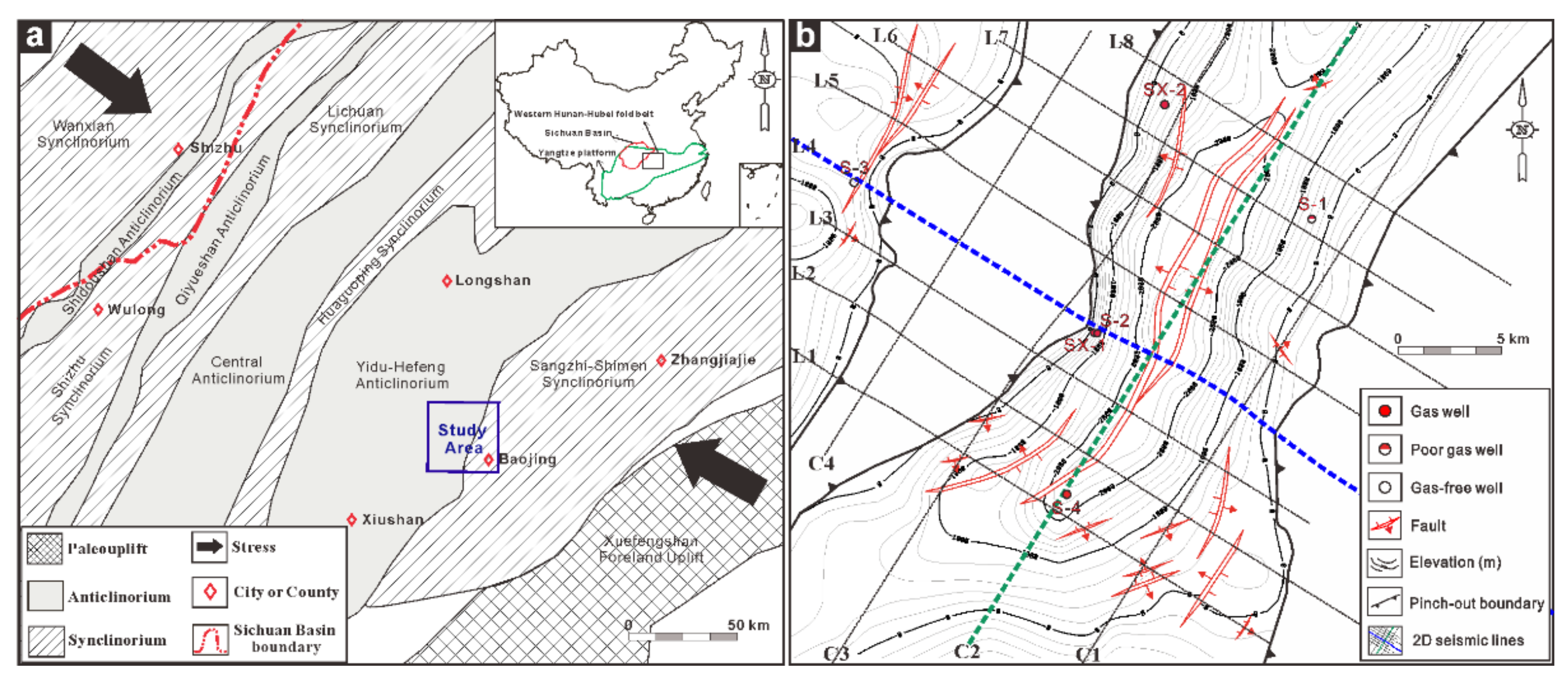
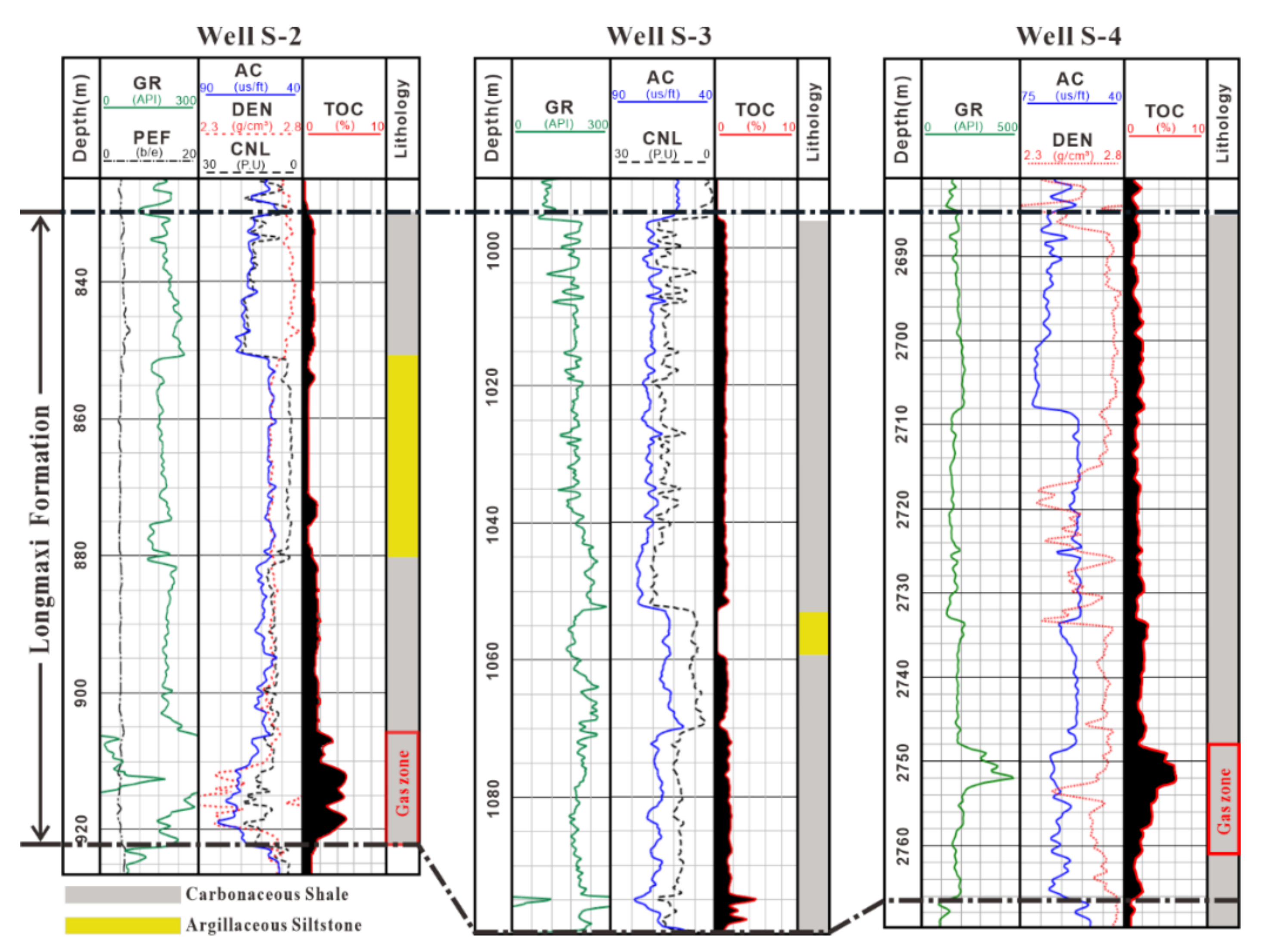
2. Target Overview
3. Methodology
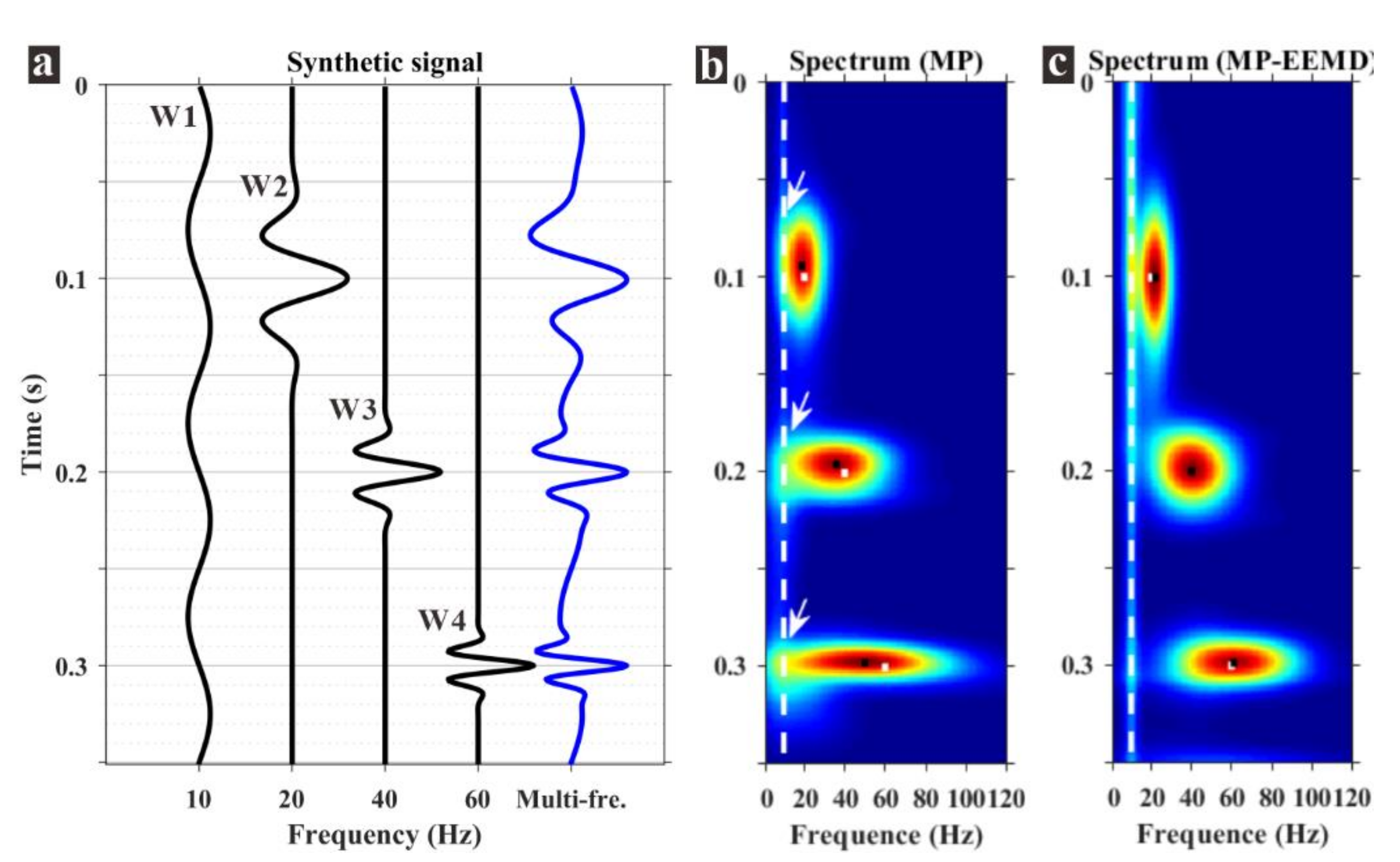
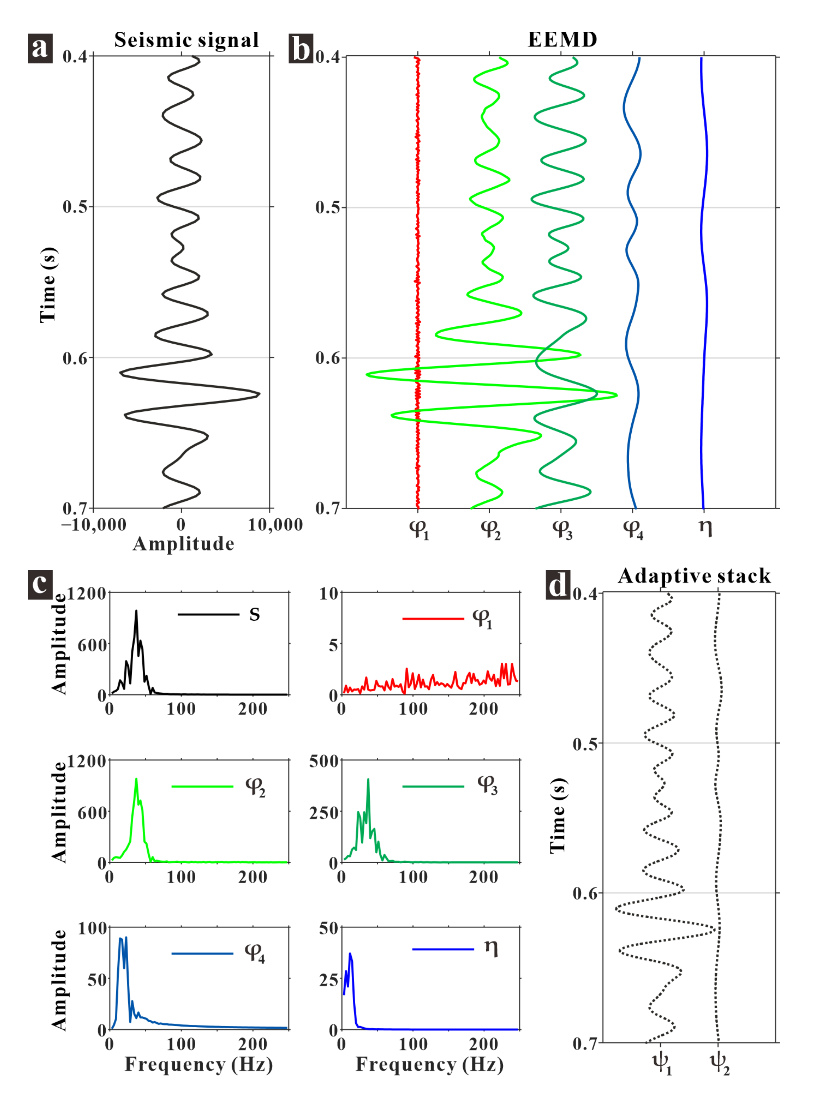
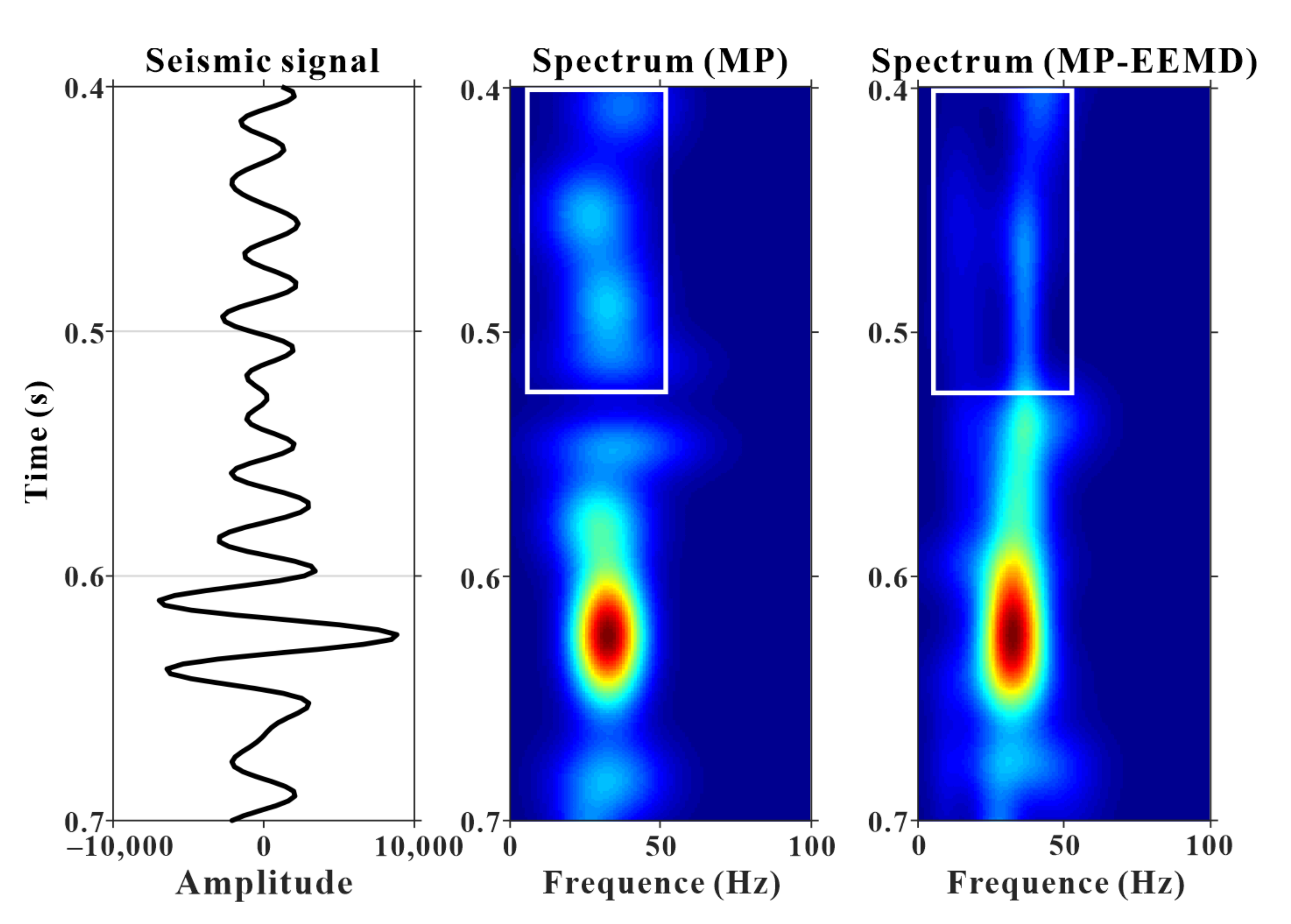
3.1. Spectral Decomposition Technology without Frequency Interference
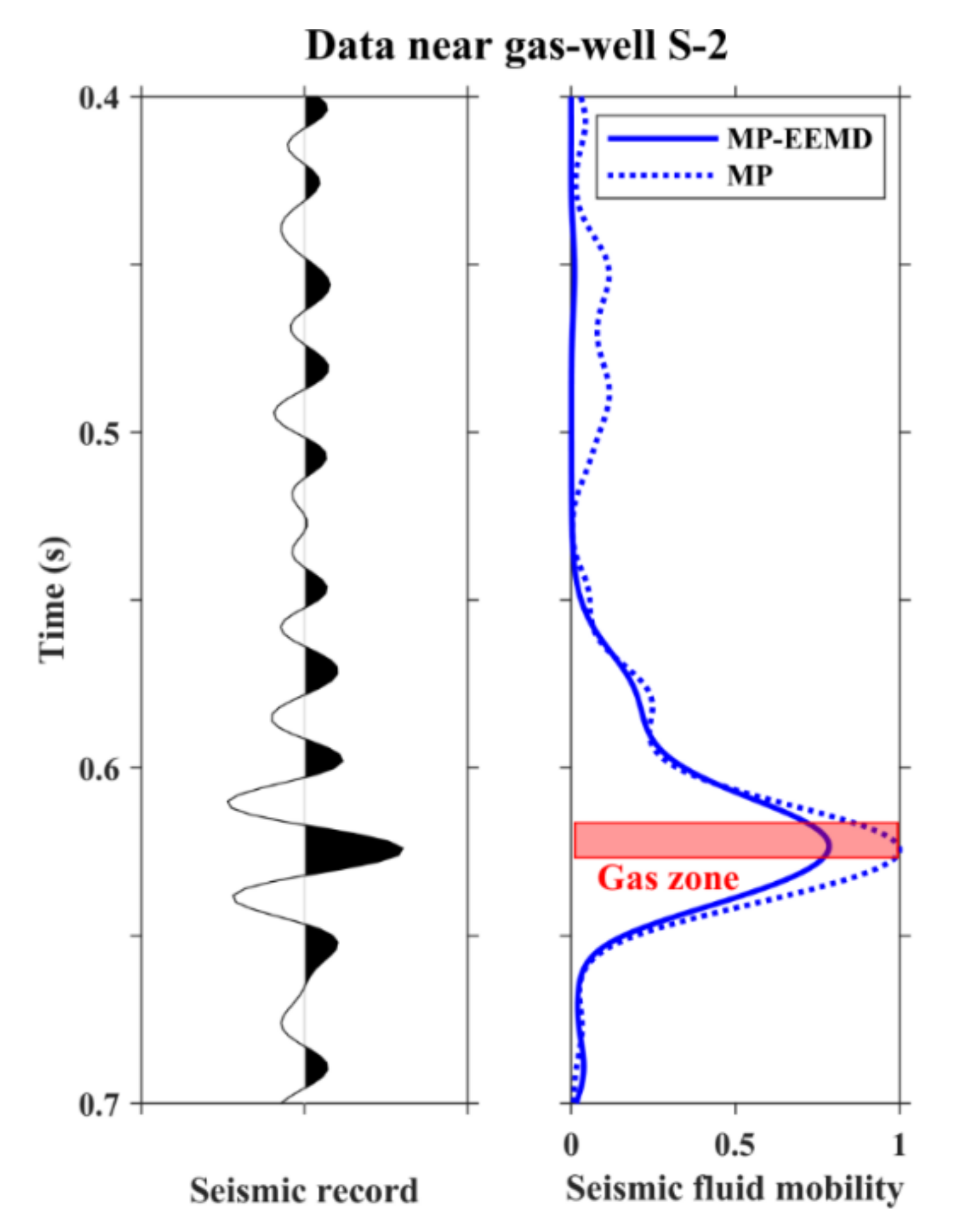
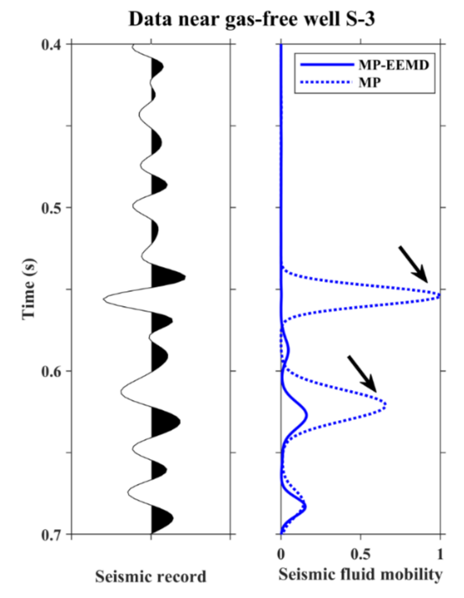
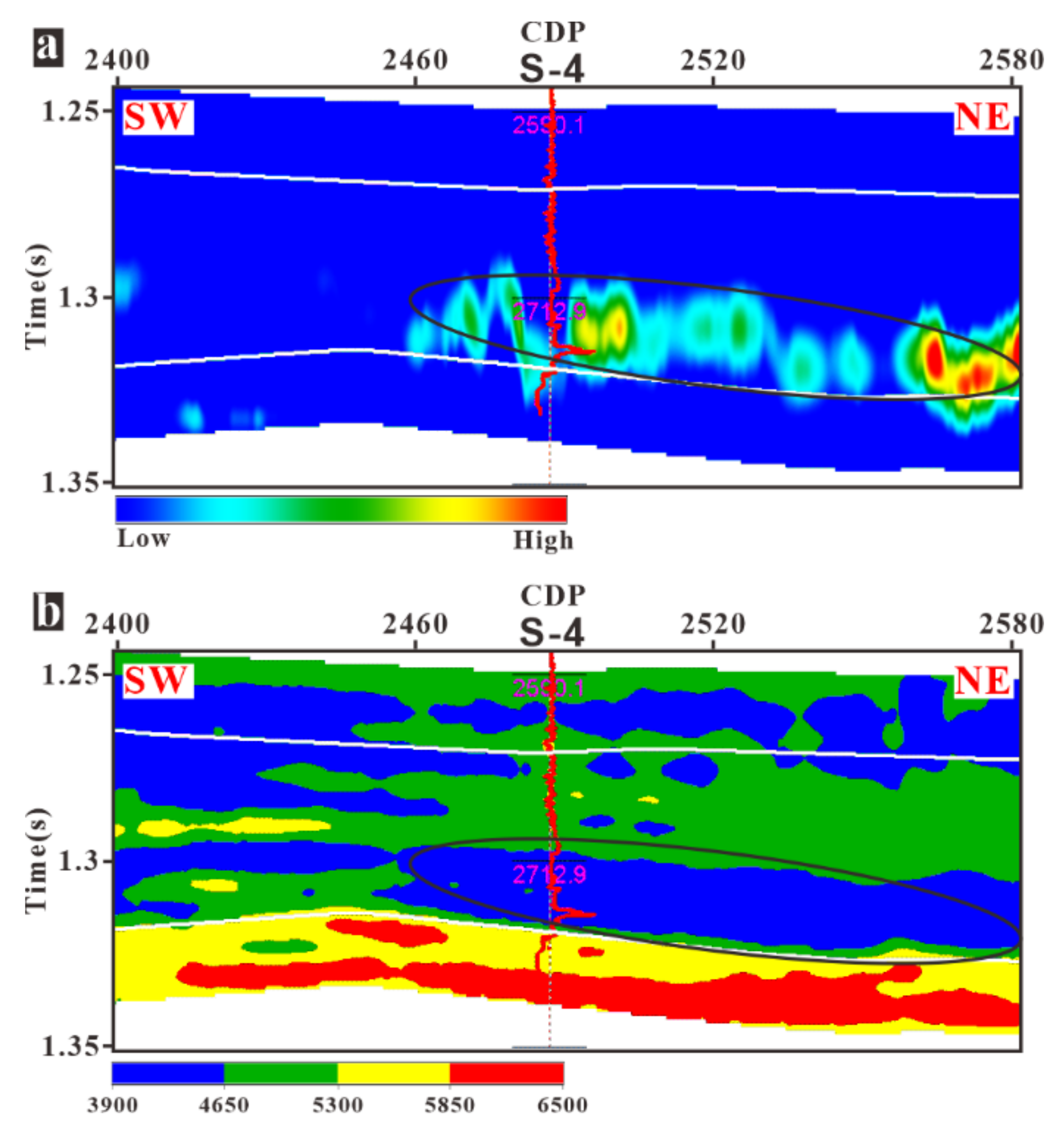
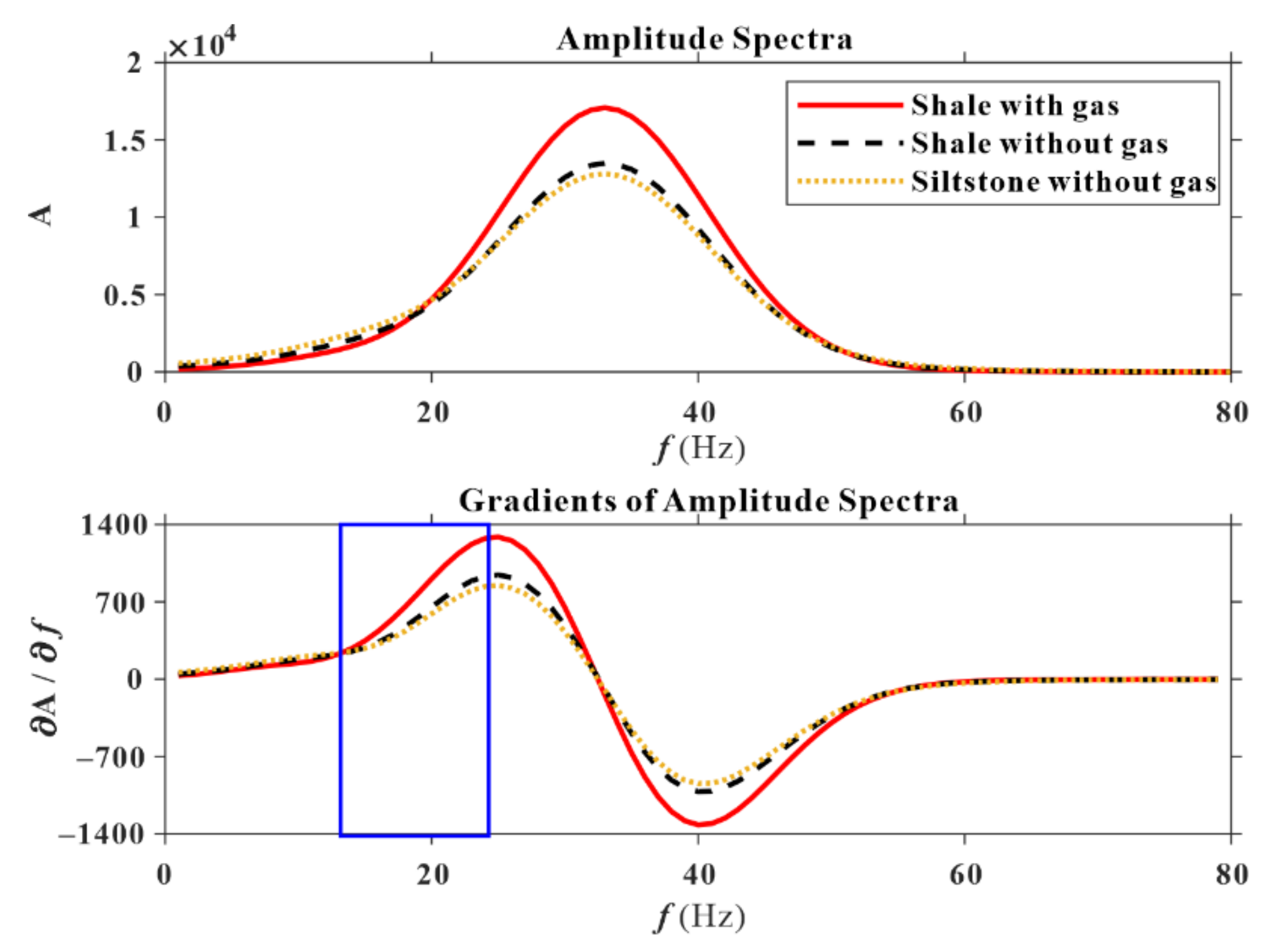
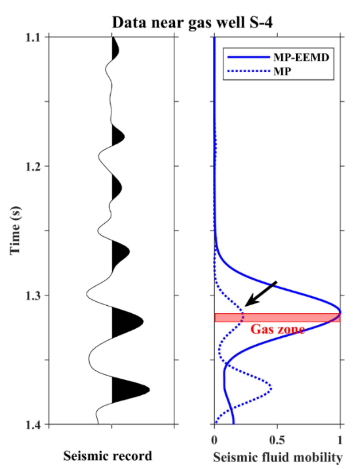
3.2. Seismic Fluid Mobility Attribute
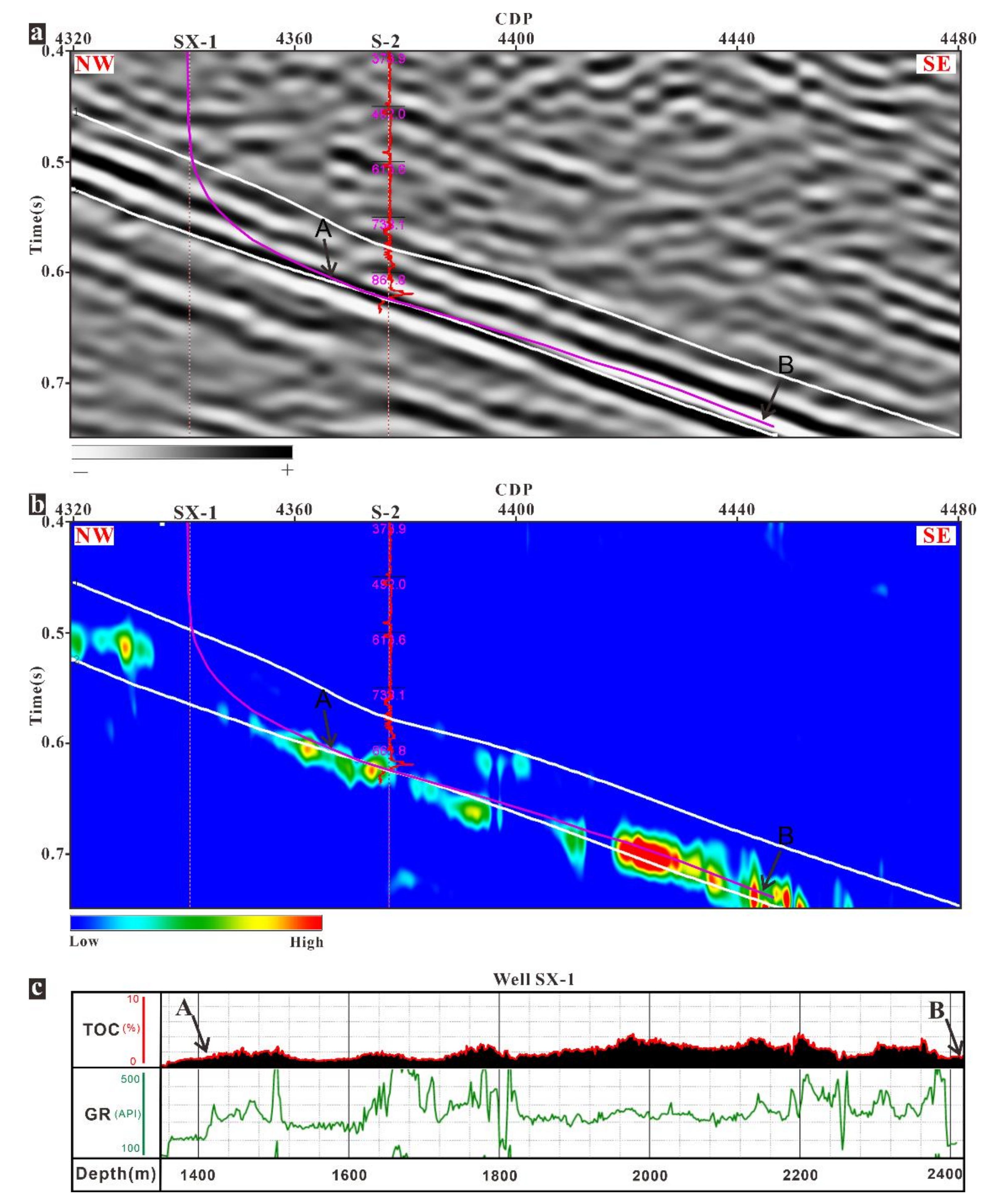
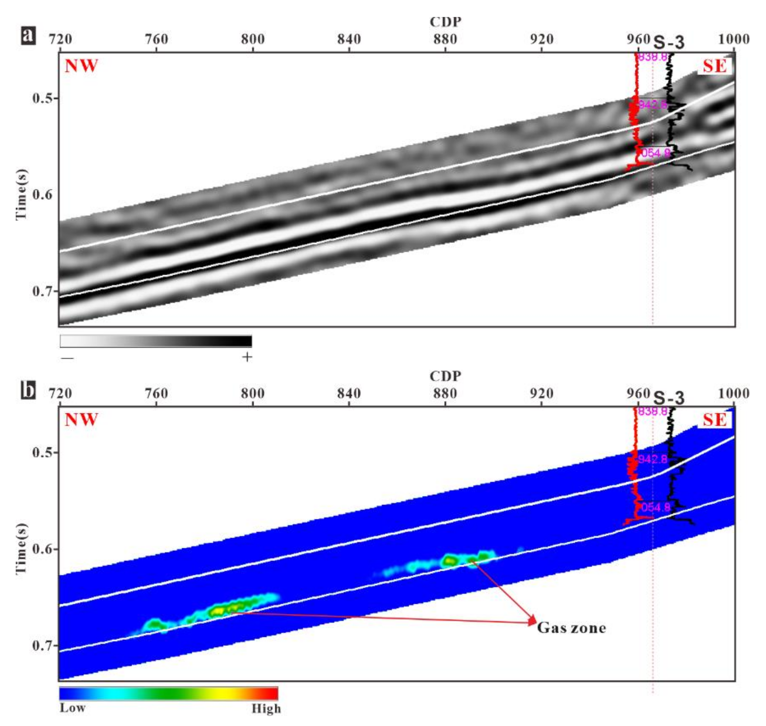
4. Results
5. Conclusions
Author Contributions
Funding
Institutional Review Board Statement
Informed Consent Statement
Data Availability Statement
Acknowledgments
Conflicts of Interest
Appendix A. Post-Stack Seismic Inversion Technology
References
- Yang, R.; He, S.; Yi, J.; Hu, Q. Nano-scale pore structure and fractal dimension of organic-rich Wufeng-Longmaxi shale from Jiaoshiba area, Sichuan Basin: Investigations using FE-SEM, gas adsorption and helium pycnometry. Mar. Pet. Geol. 2016, 70, 27–45. [Google Scholar] [CrossRef]
- Jiang, S.; Zhang, J.; Jiang, Z.; Xu, Z.; Cai, D.; Chen, L.; Wu, Y.; Zhou, D.; Jiang, Z.; Zhao, X.; et al. Geology, resource potentials, and properties of emerging and potential China shale gas and shale oil plays. Interpretation 2015, 3, SJ1–SJ13. [Google Scholar] [CrossRef]
- Xi, Z.; Tang, S.; Wang, J. The reservoir characterization and shale gas potential of the Niutitang formation: Case study of the SY well in northwest Hunan Province, South China. J. Pet. Sci. Eng. 2018, 171, 687–703. [Google Scholar] [CrossRef]
- Ma, X.; Xie, J. The progress and prospects of shale gas exploration and development in southern Sichuan Basin, SW China. Pet. Explor. Dev. 2018, 45, 172–182. [Google Scholar] [CrossRef]
- Tang, X.; Jiang, Z.; Li, Z.; Gao, Z.; Bai, Y.; Zhao, S.; Feng, J. The effect of the variation in material composition on the heterogeneous pore structure of high-maturity shale of the Silurian Longmaxi formation in the southeastern Sichuan Basin, China. J. Nat. Gas Sci. Eng. 2015, 23, 464–473. [Google Scholar] [CrossRef]
- Han, C.; Jiang, Z.; Han, M.; Wu, M.; Lin, W. The lithofacies and reservoir characteristics of the Upper Ordovician and Lower Silurian black shale in the Southern Sichuan Basin and its periphery, China. Mar. Pet. Geol. 2016, 75, 181–191. [Google Scholar] [CrossRef]
- Wang, G.; Ju, Y.; Huang, C.; Long, S.; Peng, Y. Longmaxi-Wufeng Shale lithofacies identification and 3-D modeling in the northern Fuling Gas Field, Sichuan Basin. J. Nat. Gas. Sci. Eng. 2017, 47, 59–72. [Google Scholar] [CrossRef]
- Fu, Y.; Jiang, Y.; Wang, Z.; Hu, Q.; Xie, J.; Ni, G.; Lei, Z.; Zhou, K.; Liu, X. Non-connected pores of the Longmaxi shale in southern Sichuan Basin of China. Mar. Pet. Geol. 2019, 110, 420–433. [Google Scholar] [CrossRef]
- Lee, J.; Byun, J.; Kim, B.; Yoo, D. Delineation of gas hydrate reservoirs in the Ulleung Basin using unsupervised multi-attribute clustering without well log data. J. Nat. Gas Sci. Eng. 2017, 46, 326–337. [Google Scholar] [CrossRef]
- Zeng, J.; Huang, H.; Li, H.; Miao, Y.; Wen, J.; Zhou, F. A fast complex domain-matching pursuit algorithm and its application to deep-water gas reservoir detection. J. Geophys. Eng. 2017, 14, 1335–1348. [Google Scholar] [CrossRef]
- Veeken, P.C.H.; Rauch-Davies, M. AVO attribute analysis and seismic reservoir characterization. First Break 2006, 24, 41–52. [Google Scholar] [CrossRef]
- Ross, C.P. Comparison of popular AVO attributes, AVO inversion, and calibrated AVO predictions. Lead. Edge 2002, 21, 244–252. [Google Scholar] [CrossRef]
- Castagna, J.P.; Sun, S.; Siegfried, R.W. Instantaneous spectral analysis: Detection of low-frequency shadows associated with hydrocarbons. Lead. Edge 2003, 22, 120–127. [Google Scholar] [CrossRef]
- Lichman, E.; Goloshubin, G. Unified approach to gas and fluid detection on instantaneous seismic wavelets. SEG Tech. Program Expand. Abstr. 2003, 1699–1702. [Google Scholar] [CrossRef]
- Luo, Y.; Huang, H.; Yang, Y.; Hao, Y.; Zhang, S.; Li, Q. Integrated prediction of deepwater gas reservoirs using Bayesian seismic inversion and fluid mobility attribute in the South China Sea. J. Nat. Gas Sci. Eng. 2018, 59, 56–66. [Google Scholar] [CrossRef]
- Zhang, Y.; Wen, X.; Jiang, L.; Liu, J.; Yang, J.; Liu, S. Prediction of high-quality reservoirs using the reservoir fluid mobility attribute computed from seismic data. J. Pet. Sci. Eng. 2020, 190, 107007. [Google Scholar] [CrossRef]
- Silin, D.B.; Korneev, V.A.; Goloshubin, G.M.; Patzek, T.W. A Hydrologic View on Biot’s Theory of Poroelasticity; Lawrence Berkeley National Lab. (LBNL): Berkeley, CA, USA, 2004. [Google Scholar] [CrossRef] [Green Version]
- Goloshubin, G.; Silin, D. Frequency-Dependent Seismic Reflection from a Permeable Boundary in a Fractured Reservoir; Society of Exploration Geophysicists: Tulsa, OK, USA, 2006; pp. 1742–1746. [Google Scholar] [CrossRef] [Green Version]
- Naseer, T.M.; Asim, S.; Ahmad, M.N.; Hussain, F.; Qureshi, S.N. Application of Seismic Attributes for Delineation of Channel Geometries and Analysis of Various Aspects in Terms of Lithological and Structural Perspectives of Lower Goru Formation, Pakistan. Int. J. Geosci. 2014, 5, 1490–1502. [Google Scholar] [CrossRef] [Green Version]
- Yuan, S.; Ji, Y.; Shi, P.; Zeng, J.; Gao, J.; Wang, S. Sparse Bayesian Learning-Based Seismic High-Resolution Time-Frequency Analysis. IEEE Geosci. Remote Sens. Lett. 2019, 16, 623–627. [Google Scholar] [CrossRef]
- Wang, Y. Seismic time-frequency spectral decomposition by matching pursuit. Geophysics 2007, 72, V13–V20. [Google Scholar] [CrossRef]
- Mallat, S.G.; Zhifeng, Z. Matching pursuits with time-frequency dictionaries. IEEE Trans. Signal Process. 1993, 41, 3397–3415. [Google Scholar] [CrossRef] [Green Version]
- Castagna, J.P.; Sun, S. Comparison of spectral decomposition methods. First Break 2006, 24, 75–79. [Google Scholar] [CrossRef]
- Wu, Z.; Huang, N.E. Ensemble Empirical Mode Decomposition: A Noise-Assisted Data Analysis Method. Adv. Adapt. Data Anal. 2011, 1, 1–41. [Google Scholar] [CrossRef]
- Guo, T.; Zhang, H. Formation and enrichment mode of Jiaoshiba shale gas field, Sichuan Basin. Pet. Explor. Dev. 2014, 41, 31–40. [Google Scholar] [CrossRef]
- Guo, T. Key geological issues and main controls on accumulation and enrichment of Chinese shale gas. Pet. Explor. Dev. 2016, 43, 349–359. [Google Scholar] [CrossRef]
- Wan, Y.; Tang, S.; Pan, Z. Evaluation of the shale gas potential of the lower Silurian Longmaxi Formation in northwest Hunan Province, China. Mar. Pet. Geol. 2017, 79, 159–175. [Google Scholar] [CrossRef]
- Li, Y.; Liu, H.; Zhang, L.; Lu, Z.; Li, Q.; Huang, Y. Lower limits of evaluation parameters for the lower Paleozoic Longmaxi shale gas in southern Sichuan Province. Sci. China Earth Sci. 2013, 56, 710–717. [Google Scholar] [CrossRef]
- Goloshubin, G.M.; Korneev, V.A.; Vingalov, V.M. Seismic low-frequency effects from oil-saturated reservoir zones. SEG Tech. Program Expand. Abstr. 2002, 1813–1816. [Google Scholar] [CrossRef] [Green Version]
- Huang, H.; Yuan, S.; Zhang, Y.; Zeng, J.; Mu, W. Use of nonlinear chaos inversion in predicting deep thin lithologic hydrocarbon reservoirs: A case study from the Tazhong oil field of the Tarim Basin, China. Geophysics 2016, 81, B221–B234. [Google Scholar] [CrossRef]


| NO. | Wave Equations | Parameters |
|---|---|---|
| W1 | A = 0.2, f = 10 Hz | |
| W2 | A = 1, k = 1, f = 20 Hz, u = 0.1 s | |
| W3 | A = 1, k = 1, f = 40 Hz, u = 0.2 s | |
| W4 | A = 1, k = 1, f = 60 Hz, u = 0.3 s |
Publisher’s Note: MDPI stays neutral with regard to jurisdictional claims in published maps and institutional affiliations. |
© 2020 by the authors. Licensee MDPI, Basel, Switzerland. This article is an open access article distributed under the terms and conditions of the Creative Commons Attribution (CC BY) license (http://creativecommons.org/licenses/by/4.0/).
Share and Cite
Zeng, J.; Stovas, A.; Huang, H.; Ren, L.; Tang, T. Prediction of Shale Gas Reservoirs Using Fluid Mobility Attribute Driven by Post-Stack Seismic Data: A Case Study from Southern China. Appl. Sci. 2021, 11, 219. https://doi.org/10.3390/app11010219
Zeng J, Stovas A, Huang H, Ren L, Tang T. Prediction of Shale Gas Reservoirs Using Fluid Mobility Attribute Driven by Post-Stack Seismic Data: A Case Study from Southern China. Applied Sciences. 2021; 11(1):219. https://doi.org/10.3390/app11010219
Chicago/Turabian StyleZeng, Jing, Alexey Stovas, Handong Huang, Lixia Ren, and Tianlei Tang. 2021. "Prediction of Shale Gas Reservoirs Using Fluid Mobility Attribute Driven by Post-Stack Seismic Data: A Case Study from Southern China" Applied Sciences 11, no. 1: 219. https://doi.org/10.3390/app11010219
APA StyleZeng, J., Stovas, A., Huang, H., Ren, L., & Tang, T. (2021). Prediction of Shale Gas Reservoirs Using Fluid Mobility Attribute Driven by Post-Stack Seismic Data: A Case Study from Southern China. Applied Sciences, 11(1), 219. https://doi.org/10.3390/app11010219