Numerical Investigation of Stable Stratification Effects on Wind Resource Assessment in Complex Terrain

Abstract

In the present study, we perform numerical simulations considering various stable atmospheric conditions for a small-scale simple topography. Based on the obtained simulation results, we visualize the flow field and discuss drastic changes in the flow patterns. A flow pattern similar to the potential flow suddenly appears around an isolated hill as the stability increases, regardless of the inclination angle of the hill. We show that a critical Richardson number clearly exists. Furthermore, the effect of stable stratification on the evaluation of power generation is shown for typical complex terrain. We evaluate the capacity factor (%) of a 2 MW large wind turbine based on one-year virtual mast data and consider the effect of stable stratification. It is shown, in the case of stable stratification, that the capacity factor is 2.775 times greater than that under neutral stratification.

1. Introduction

The atmospheric boundary layer generally forms a stratified state, in which the density or temperature changes in the vertical direction [1]. In particular, the flow in the surface inversion layer that appears at night forms a stable stratified flow, in which the density decreases and the temperature increases with height. Negative buoyancy forces act on the flow field when stable stratified flows pass through complex terrain. As a result, as shown in Figure 1 (which is the computational fluid dynamics (CFD) simulation results based on large eddy simulation by the first author), there are drastic changes between the flow patterns under neutral stratification (Froude number—Fr = 1000) and stable stratification (Fr = 0.1). From the above, it is extremely important to numerically predict airflow characteristics over complex topographies under stable stratifications in relation to the effective use of wind energy [2,3,4,5], the prediction of advection-diffusion phenomena of air pollutants [6,7], the topographically enhanced local severe wind problem [8,9], and so on. Our recent research area is wind power generation. For the literature review on wind turbines, details are organized in two recent papers [10,11].

The main purpose of this study is to clarify stable stratification effects on wind resource assessment in complex terrains, especially in the field of wind power generation. For this purpose, computational fluid dynamics (CFD) simulations based on large eddy simulation were used here; in addition, a detailed numerical investigation was carried out using the obtained numerical results.

First, the CFD simulation was performed by selecting an isolated hill as a simple terrain scenario. In particular, we conducted a detailed numerical study of the effects of the spatial resolution of the computational grid used in this study, along with various inflow profiles, wide-range atmospheric stability, and the topographic inclination angle of the hill.

Next, the numerical investigation of stable stratification effects on wind resource assessment in complex terrain was performed. Two types of CFD simulations were performed under neutral and stable stratification conditions, targeting complex terrain featuring large 2 MW wind turbines. The numerical results for both cases were compared, along with the flow fields formed around the wind turbines. The effect of the difference in atmospheric stability on the flow fields was also considered. Furthermore, we evaluated the economic efficiency of large wind turbines based on one-year virtual mast data and examine the effect of stable stratification on the capacity factor (%).

2. Summary of the Numerical Simulation Methods

An isolated hill was selected as a simple terrain scenario and CFD simulation was performed using this topography. In particular, we conducted a detailed numerical study of the effects of the spatial resolution of the computational grid, various inflow profiles, wide-range atmospheric stability, and the topographic inclination angle. We used the RIAM-COMPACT CFD model [12,13,14,15]. Our papers [12,13,14,15] mainly conducted the LES (large eddy simulation) investigation of terrain-induced turbulence in complex terrain and discussed the turbulence generation mechanism. The numerical simulation method was based on the finite difference method, while LES was adopted for the turbulence model.

With the LES approach, a spatial filter was applied to the flow field. As a result, turbulent vortices of various sizes were separated into GS (grid scale) components, which were larger than the computational grid, and SGS (sub-grid scale) components, which were smaller than the computational grid. Large-scale vortices of GS components were directly numerically simulated without relying on a model. On the other hand, the energy dissipation effect of small-scale vortices on SGS components was modeled based on physical consideration of the SGS stress. The governing equations of flow were the continuity equation of the filtered incompressible fluid, the Navier–Stokes equation, the Boussinesq approximation, and the energy equation (temperature equation). The standard Smagolinsky model [16] was used for the LES SGS model. The wall damping function was also used, where the model coefficient was set to 0.1. The governing equations used in this study are shown below:

$$\frac{\partial {\overline{\mathrm{u}}}_{\mathrm{i}}}{\partial {\mathrm{x}}_{\mathrm{i}}}=0$$

(1)

$$\frac{\partial {\overline{\mathrm{u}}}_{\mathrm{i}}}{\partial \mathrm{t}}+{\overline{\mathrm{u}}}_{\mathrm{j}}\frac{\partial {\overline{\mathrm{u}}}_{\mathrm{i}}}{\partial {\mathrm{x}}_{\mathrm{j}}}=-\frac{\partial \overline{\mathrm{p}}}{\partial {\mathrm{x}}_{\mathrm{i}}}+\frac{1}{\mathrm{Re}}\frac{{\partial }^2{\overline{\mathrm{u}}}_{\mathrm{i}}}{\partial {\mathrm{x}}_{\mathrm{j}}\partial x_j}-\frac{\partial {\mathsf{\tau }}_{\mathrm{i}\mathrm{j}}}{\partial {\mathrm{x}}_{\mathrm{j}}}+{\mathrm{R}}_{\mathrm{i}}\overline{\mathsf{\theta }} {\mathsf{\delta }}_{\mathrm{i}3}$$

(2)

$$\frac{\partial \overline{\mathsf{\theta }}}{\partial \mathrm{t}}+{\overline{\mathrm{u}}}_{\mathrm{j}}\frac{\partial \overline{\mathsf{\theta }}}{\partial {\mathrm{x}}_{\mathrm{j}}}=\frac{1}{\mathrm{RePr}}\frac{{\partial }^2\overline{\mathsf{\theta }}}{\partial {\mathrm{x}}_{\mathrm{j}}\partial {\mathrm{x}}_{\mathrm{j}}}-\frac{\partial {\mathrm{h}}_{\mathrm{j}}}{\partial {\mathrm{x}}_{\mathrm{j}}}$$

(3)

$${\mathsf{\tau }}_{\mathrm{ij}}-\frac{1}{3}{\mathsf{\delta }}_{\mathrm{ij}}{\mathsf{\tau }}_{\mathrm{kk}}=-2{\mathsf{\nu }}_{\mathrm{SGS}}{\overline{\mathrm{S}}}_{\mathrm{ij}}$$

(4)

$${\overline{\mathrm{S}}}_{\mathrm{ij}}=\frac{1}{2}\left(\frac{\partial {\overline{\mathrm{u}}}_{\mathrm{i}}}{\partial {\mathrm{x}}_{\mathrm{j}}}+\frac{\partial {\overline{\mathrm{u}}}_{\mathrm{j}}}{\partial {\mathrm{x}}_{\mathrm{i}}}\right)$$

(5)

$${\mathrm{h}}_{\mathrm{j}}=-{\mathsf{\alpha }}_{\mathrm{SGS}}\frac{\partial \overline{\mathsf{\theta }}}{\partial {\mathrm{x}}_{\mathrm{j}}}$$

(6)

$${\mathsf{\alpha }}_{\mathrm{SGS}}=\frac{{\mathsf{\nu }}_{\mathrm{SGS}}}{{\mathrm{Pr}}_{\mathrm{SGS}}}$$

(7)

In the CFD simulation of the temperature stratification flow, the Richardson number, Ri—a dimensionless parameter representing atmospheric stability—is defined as follows:

$${\mathrm{R}}_{\mathrm{i}}=\frac{\mathrm{g}\left({\mathsf{\theta }}_{\mathrm{in}}-{\mathsf{\theta }}_{\mathrm{bottom}}\right)\mathrm{h}}{{\mathsf{\theta }}_{\mathrm{in}}{\mathrm{U}}^2}$$

(8)

The Reynolds number, which is a dimensionless parameter used in Equation (2), is defined as follows:

$$\mathrm{Re}=\frac{\mathrm{Uh}}{\mathsf{\nu }}$$

(9)

In Equation (3), Pr_SGS was set to 0.5. Furthermore, in Equation (8), ${\mathsf{\theta }}_{\mathrm{in}}$ is the inflow temperature, ${\mathsf{\theta }}_{\mathrm{bottom}}$ is the ground temperature, U is the inflow wind speed, h is the representative length, and g is gravitational acceleration. In Equation (9), ν is the kinematic viscosity coefficient. The Reynolds number was set to 10⁴ in the present study.

The numerical algorithm used was based on the fractional step method [17]. The Euler explicit method was used as the time integration method. The Poisson equation for pressure was solved by the successive over-relaxation method. The discretization of spatial terms only featured second-order central difference schemes, except for the convective term of the Navier–Stokes equation. Here, Kajishima’s interpolation method [18] was used for the fourth-order central difference scheme, which composes the convection term. The weight of the numerical diffusion term of the third-order upwind scheme was set to α = 0.5—with respect to α = 3.0 of the normal Kawamura–Kuwahara scheme type [19]—and its influence was sufficiently small.

3. CFD Simulation for the Isolated Hill Scenario

First, an isolated hill was selected as a simple terrain scenario. Then, CFD simulation was performed for this topography. In particular, we conducted a detailed numerical investigation of the effects of the spatial resolution of the computational grid, various inflow profiles, wide-range atmospheric stability, and the topographic inclination angle.

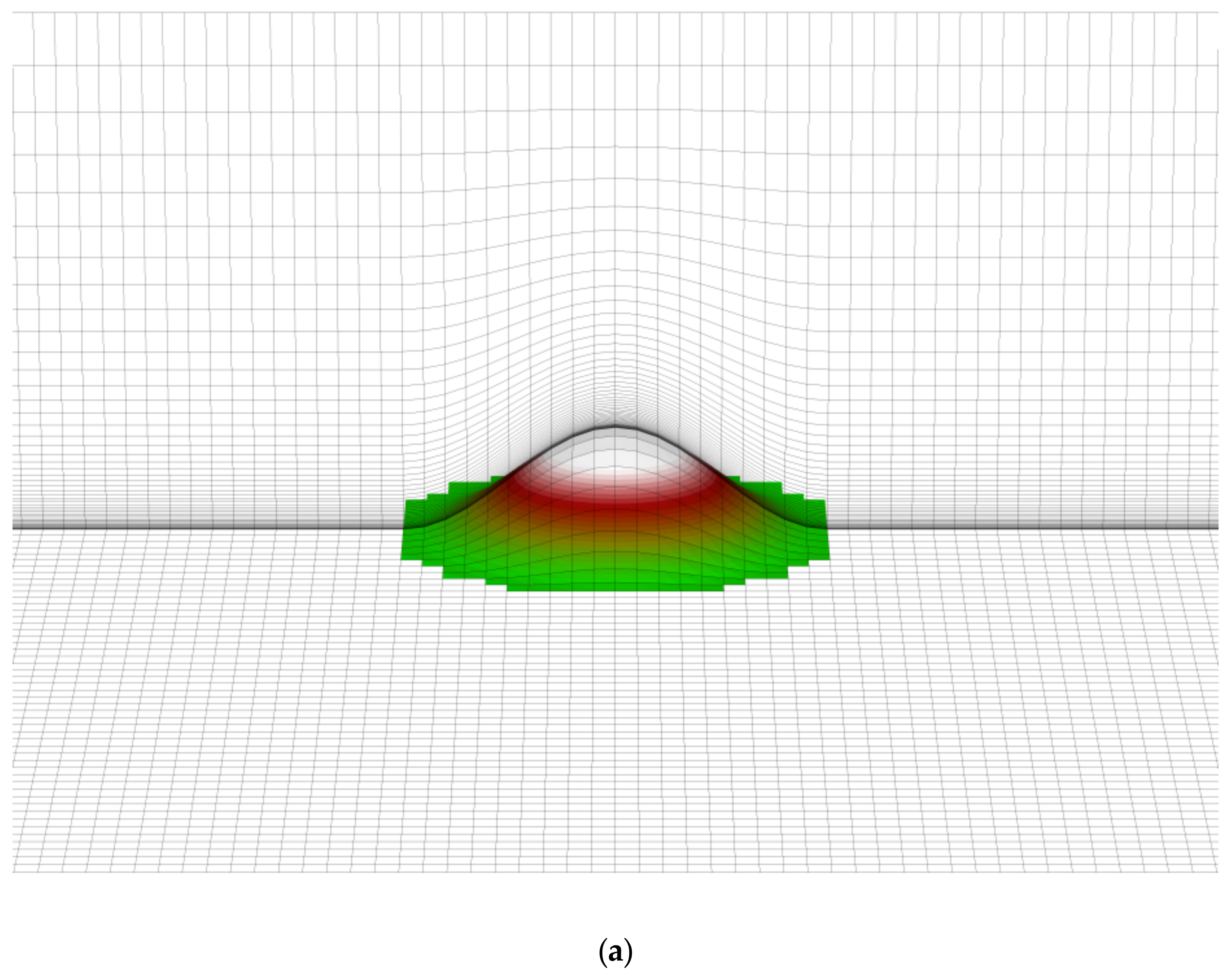
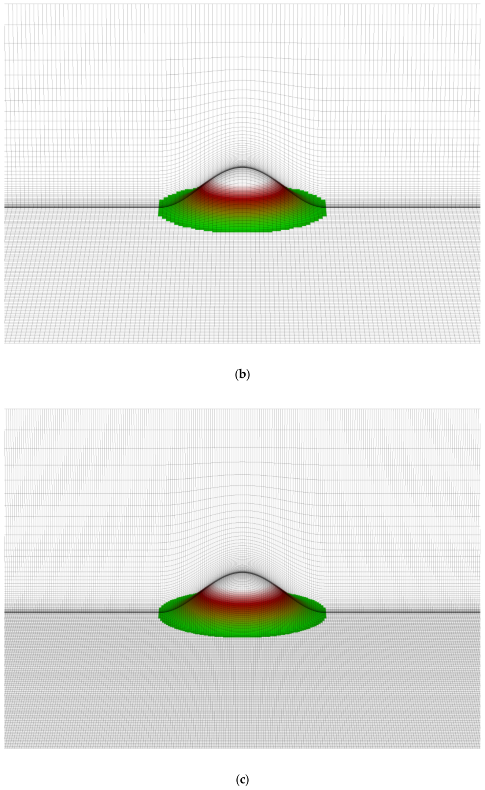
3.1. Effects of the Grid Resolution on the Numerical Results for the Steep Isolated Hill Scenario

Figure 2 shows the computational domain, co-ordinate system, and boundary conditions used in this study. In all simulations in this study, the initial condition of the flow was impulsively started from rest. As shown in the figure, the shape of the isolated hill is expressed by the cosine function shown below. We used two values for the variable a (a = 2 h and 10 h) in order to reproduce steep and gentle hills. Here, r is the horizontal distance from the origin. We prepared three types of computational grids with different horizontal spatial resolutions. Figure 3 shows a comparison of the computational grids near the isolated hill. Here, with the three types of computational grids, the number of grids in the vertical direction and the spatial resolution were set to have the same values. In this section, the value for a in Equation (10) was set to 2 h and the steep hill scenario was used as the simulation target.

$$\mathrm{If} \mathrm{r}\le \mathrm{a}, \mathrm{then} \mathrm{z}\left(\mathrm{r}\right) = 0.5 \mathrm{h} \times \{1+\cos (\mathsf{\pi }\mathrm{r}/\mathrm{a})\}, \mathrm{and} \mathrm{if} \mathrm{r}>\mathrm{a}, \mathrm{then} \mathrm{z}\left(\mathrm{r}\right)=0$$

(10)

In order to outline the unsteady flow pattern formed around the isolated hill under neutral stratification, Figure 4 shows a comparison of flow visualization in wind tunnel experiments and CFD simulation results. In the wind tunnel experiment, the flow field was visualized using the smoke wire method. On the other hand, in the CFD simulation, the flow field was visualized using the passive particle tracking method based on the numerical results using the medium grid shown in Figure 3b. In both cases, uniform flow was imposed as the inflow condition. It can be seen that very similar flow patterns were formed in both the wind tunnel experiment and the CFD simulation; that is, an isolated vortex was formed near the hilltop, later forming a large-scale vortex (backflow region) behind the hill. The large-scale vortex periodically shed to the downstream side of the hill and flowed downwards. We have already compared the RANS (Reynolds-Averaged Navier-Stokes) results and the present LES results in past paper [20]. Furthermore, we have also conducted wind tunnel experiments using a scale model in the past, and have completed the verification of the prediction accuracy of the LES approach adopted in this study [21,22]. In the wind tunnel experiment [21,22], in order to confirm the reproducibility of the flow pattern, the shape of the target model was changed and airflow measurements were carried out more than a dozen times over multiple years.

The following presents a comparison of the numerical results using the three computational grids shown in Figure 3. Here, the atmospheric stability was set to the neutral stratified state, while the inflow condition was imposed by shear flow with a power law index of N = 7. Figure 5 shows a comparison of the streamlines for a time-averaged flow field near the hill. Pay attention to the central position of the vortex region formed behind the isolated hill. Using the coarse grid, the numerical results (shown in Figure 5a) were located slightly downstream of those in Figure 5b,c, but similar results were obtained. Here, Figure 5b shows the numerical result using the medium grid and Figure 5c shows the numerical result using the fine grid. Figure 6 shows a comparison of the time-averaged U-velocity at a measurement station (x = 2 h) behind the steep hill. The measurement station is shown in Figure 5. This is a point where it is very difficult to predict the wind velocity distribution because it is strongly affected by the separation flow generated behind the hill. Through this result, no significant difference in the numerical results was found for the three types of computational grids and all the numerical results showed almost the same tendency. From the above, in advance, we confirmed the effect of the spatial resolution of the three types of computational grids on the flow field formed around the steep isolated hill. After that, we decided to use the medium grid shown in Figure 3b.

3.2. Effects of the Inflow Profiles on the Numerical Results for the Steep Isolated Hill Scenario

We conducted a detailed numerical investigation of the effects of various inflow profiles on the numerical results for the flow field passing over the steep isolated hill. Figure 7 shows a comparison of flow patterns for a time-averaged flow field under various inflow conditions in the case of the steep hill scenario. In all cases, a backflow region was formed behind the isolated hill. Its size was almost always the same, regardless of the difference in inflow profile. In order to consider this result more quantitatively, Figure 8 shows the comparison of a time-averaged U-velocity at a measurement station (x = 2 h) behind the steep hill under various inflow conditions. From this result, it is clearly shown that a difference in the inflow profile does not result in a significant difference in the flow phenomenon in the backflow region formed behind the isolated hill.

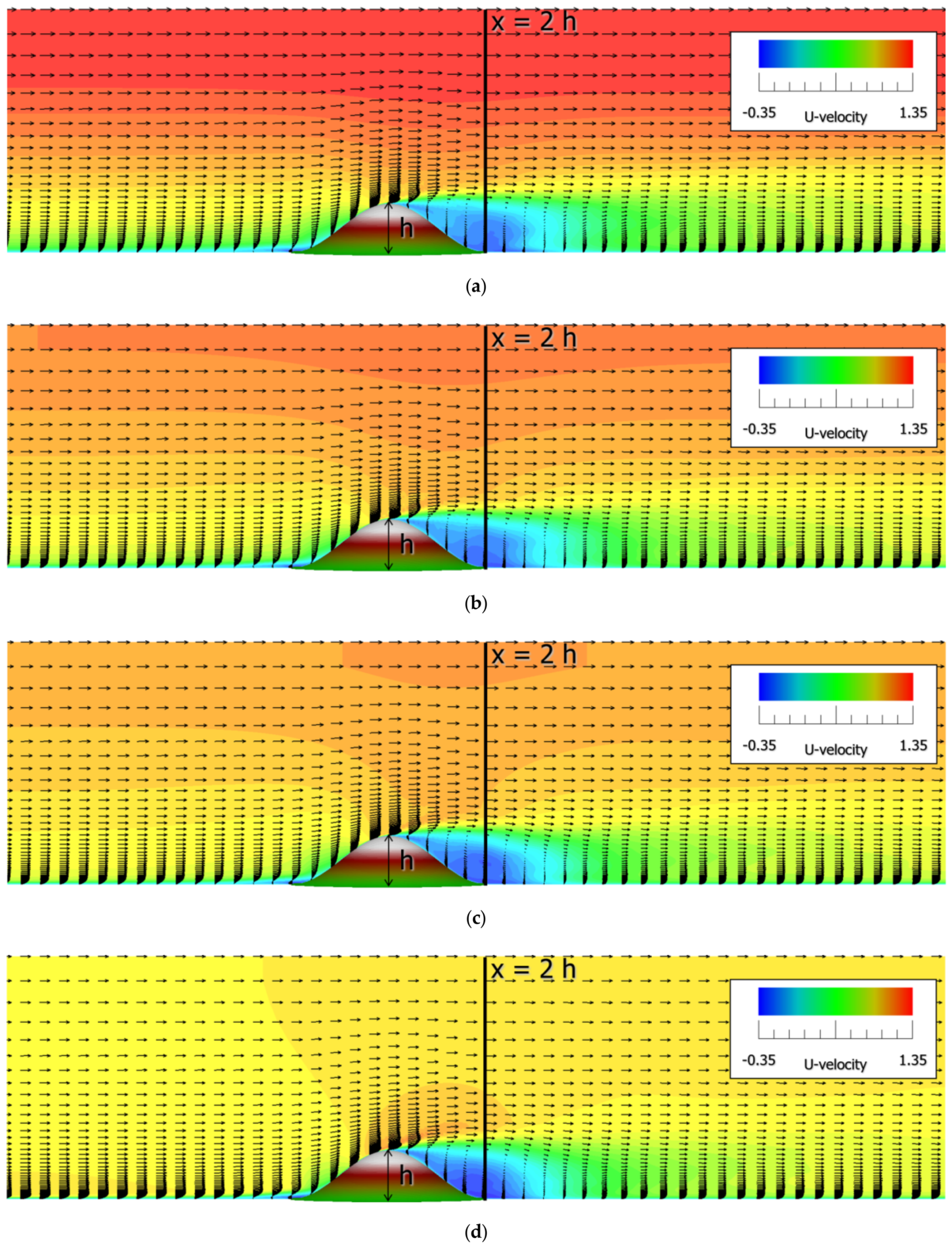
3.3. Effect of Atmospheric Stability on the Numerical Results for the Steep Isolated Hill Scenario

CFD simulations were performed considering a wide range of atmospheric stability. Shear flow with power law index N = 7 was imposed on the inflow conditions. We investigated the type of changes occurring in the flow field that passes over the steep isolated hill as the atmospheric stability gradually increases from the neutral stratified state to the stable stratified state. Figure 9 shows a comparison of flow patterns for an instantaneous flow field under various stable conditions in the case of the steep hill scenario. Figure 10 shows a comparison of flow patterns for a time-averaged flow field under various stable conditions in the case of the steep hill scenario, corresponding to Figure 9. Furthermore, Figure 11 shows a comparison of enlarged views near the hill corresponding to Figure 10. By comparing these numerical results, it is clear that, as the atmospheric stability gradually increases, the periodic large-scale vortex shedding from the isolated hill is gradually suppressed, which can be clearly observed under neutral stratification. What should be noted here is that, when Ri was above 0.5, the periodic large-scale vortex shedding from the isolated hill suddenly disappeared and a flow pattern similar to the potential flow appeared around the hill. In other words, the flow pattern which formed around the isolated hill with Ri = 0.5 showed a drastic change and it was clear that a critical Richardson number exists for flow around the hill. The detailed examination of the critical Richardson number was carried out in the Appendix A.

For further quantitative consideration, Figure 12 shows a comparison of the time-averaged U-velocity under various stable conditions at the top of the isolated hill (x = 0 h) and downstream of the hill (x = 2 h). Pay attention to the behavior of the time-averaged U-velocity at the top of the hill (x = 0 h), as shown in Figure 12a. As the atmospheric stability increased, the rate of local acceleration gradually increased. At the same time, the position of occurrence tended to approach the hill surface (see Figure 13). What should be noted here is that, as mentioned earlier, there was a drastic change in the behavior of the U-velocity when Ri exceeded 0.5. At Ri = 0.6 and 1.0, a larger acceleration effect was obtained, as compared to the case where Ri ≤ 0.5 (see Figure 13). This is because, as mentioned earlier, at Ri = 0.6 and 1.0, the periodic large-scale vortex shedding from the isolated hill disappeared suddenly and a flow pattern similar to the potential flow appeared around the hill. On the other hand, we paid attention to the behavior of the time-averaged U-velocity downstream of the isolated hill (x = 2 h). From this figure, it is clear that at Ri = 0.6 and 1.0, the periodic large-scale vortex shedding from the isolated hill disappeared. As a result, the backflow region was not formed and a flow pattern similar to the potential flow.

Figure 14 shows a comparison of surface flow patterns for a time-averaged flow field in the case of the steep hill scenario. As mentioned earlier, near the top of the hill (x = 0 h), the stable stratified flow case (Ri = 1.0)—shown in Figure 14b—has a larger acceleration effect, when compared with the neutral flow case (Ri = 0.0) shown in Figure 14a. At the same time, it can be seen that the generation area was very wide. On the other hand, in the downstream region of the isolated hill (x = 2 h), the backflow region that was clearly observed in neutral flow case (Ri = 0.0) disappeared in the stable stratified flow case (Ri = 1.0), as shown in Figure 14b. As a result, it can be seen that a forward flow region was formed. It was also confirmed that a local acceleration region was formed at x ≥ 2 h, downstream of the hill.

3.4. Effect of the Inflow Profile on the Numerical Results for the Gentle Isolated Hill Scenario

Here, we explain the results of examining the effects of various inflow profiles on the numerical results for the flow field scenario of flowing past a gentle hill. Figure 15 shows the comparison of flow patterns for a time-averaged flow field under various inflow conditions in the case of the gentle hill. Figure 16 shows a comparison of time-averaged U-velocities at a measurement station (x = 10 h) behind the gentle hill under neutral conditions. Here, the position of x = 10 h is shown in Figure 15. Focusing on the region behind the topography in Figure 15, it is shown that there were no clearly observable backflow regions in all cases of the steep hill scenario and that a deceleration region was formed. Focusing on Figure 16, the time-averaged U-velocity behaved almost the same at N = 4, 7, and 10. However, it was shown that the uniform flow results showed a larger velocity distribution in the range affected by the hill, when compared to the other results.

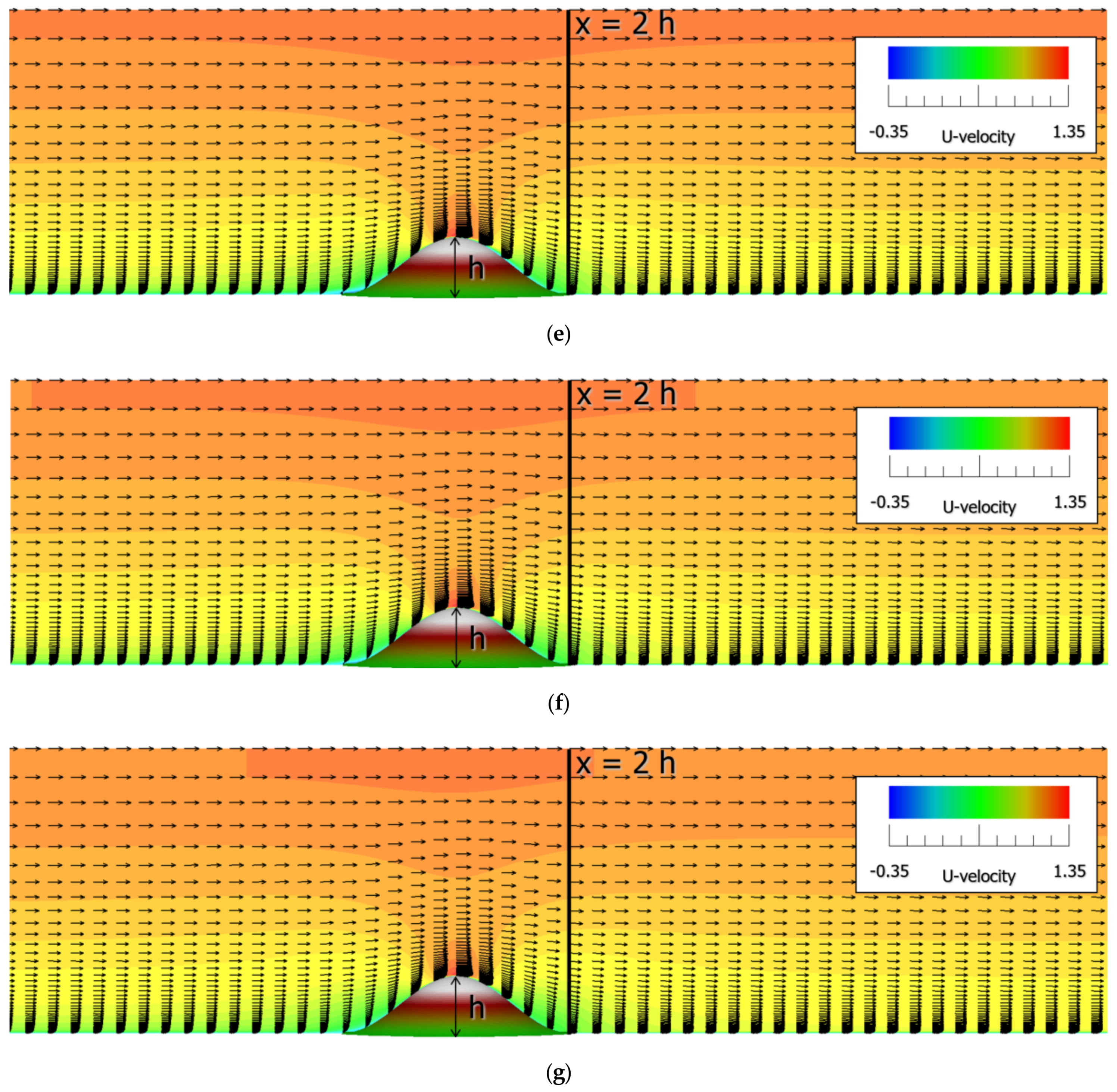
3.5. Effect of Atmospheric Stability on the Numerical Results for the Gentle Isolated Hill Scenario

CFD simulations were performed, considering a wide range of atmospheric stability values for the flow field past the gentle hill. Shear flow with power law index N = 7 was imposed on the inflow conditions. We investigated the types of changes that occurred around the flow field past the gentle hill as the atmospheric stability gradually increased from the neutral stratified state to the stable stratified state. Figure 17 shows a comparison of flow patterns for a time-averaged flow field under various stable conditions in the case of the gentle hill. Similar to the steep hill scenario explained earlier, it can be seen that a flow pattern similar to the potential flow appeared around the isolated peak as the atmospheric stability increased. It was found that a critical Richardson number clearly existed in the case of the gentle hill, as well as in the case of the steep hill. This will be described in more detail in Section 3.6.

Figure 18 shows the comparison of surface flow patterns for a time-averaged flow field in the case of the gentle hill scenario. Compared with the neutral flow case (Ri = 0.0) shown in Figure 18a, it can be seen that a drastic change occurred in the stable stratified flow case (Ri = 1.0) shown in Figure 18b. In the stable stratified flow case (Ri = 1.0) shown in Figure 18b, no backflow or deceleration of flow was observed in a wide range, from the top of the isolated hill (x = 0 h) to the downstream area. In addition, it was revealed that the flow near the topographic surface was locally accelerated.

3.6. Effect of Continuously Changing Atmospheric Stability on the Numerical Results for the Gentle Isolated Hill Scenario

We performed a CFD simulation where the Ri number was continuously changed from 0.0 (neutral flow) to 1.0 (stable stratified flow) for the flow field passing over the gentle hill. Shear flow with power law index N = 7 was imposed on the inflow conditions. The behavior of the obtained flow field was observed in detail. In this CFD simulation, Ri = 0.0 (neutral flow), dimensionless time unit of 100, and a sufficiently developed flow field were used for the initial conditions, then Ri was continuously changed to 1.0 (stable stratified flow). The results that were obtained are shown in Figure 19. In particular, three measurement points with different heights of z = 0.003, 0.05, and 0.1 h were set downstream of the isolated hill (x = 10 h). At these measurement points, the U-velocity time change was observed together with the time change of the Ri number. Careful observation of Figure 19 shows drastic changes in the U-velocity at the three measurement points of z = 0.003, 0.05, and 0.1 h at dimensionless time unit 135 (i.e., around Ri = 0.3). In other words, the effect of stable stratification on the flow field around the hill was not so remarkable, in terms of the time period before the dimensionless time unit 135 (i.e., Ri < 0.3). As a result, the flow behind the hill fluctuated significantly over time. On the other hand, after dimensionless time unit 135 (i.e., when Ri ≥ 0.3), the effect of stable stratification became remarkable, in terms of affecting the flow around the hill. As mentioned earlier, a flow pattern similar to the potential flow suddenly appeared around the isolated hill. Therefore, as with the steep hill, a critical Richardson number was clearly present for the flow field passing over the gentle hill. Its value was shown to be about 0.3. The detailed examination of the critical Richardson number for the steep isolated hill was carried out in the Appendix A.

4. CFD Simulation for Complex Terrain

Next, we discuss the effect of stable stratification in a virtual situation where two 2 MW wind turbines (hub height of 78 m and rotor diameter of 80 m) were installed in series on real complex terrain of the Kyushu region of Japan. Here, the physical model that reproduces the wind turbine wake is not considered. That is, it simply assumes the existence of a wind turbine. The results of the CFD simulation are shown below, with Ri = 0.0 in the neutrally stratified state and Ri = +1.0 in the strongly stable stratified state. As shown in Figure 20, the separation distance between the two wind turbines was 1480 m. The altitude of the wind turbine on the downstream side was about 200 m lower than the altitude of the wind turbine on the upstream side. From now on, for convenience, the downstream wind turbine will be referred to as the No. 2 wind turbine and the upstream wind turbine will be referred to as the No. 1 wind turbine. We also assumed a virtual met mast with a height of 50 m right next to the No. 1 wind turbine. The shape of the complex terrain was constructed based on the 10 m elevation data of the Geospatial Information Authority of Japan and changes in topographical undulations were reflected as boundary conditions for the CFD simulation. The ground surface roughness was not considered in the CFD simulation. In addition, the inflow conditions were the same as in the case of the isolated hill scenario, while inflow fluctuations were not taken into consideration. We focused on the topographical effects and the effect of atmospheric stability on the airflow characteristics in the swept area of the wind turbine. The purpose of this study is to clarify the effects of both of the above.

Figure 21 shows the spatial distribution (side view) of the U-velocity in the vertical cross-section passing through the No. 1 wind turbine and the No. 2 wind turbine for the instantaneous field at dimensionless time 100, in which the flow field was fully developed. At Ri = 0.0, in the neutral stratified state shown in Figure 21a, it can be seen that the flow separates from the upstream corner of the topography and that the separated flow affects the entire No. 2 wind turbine. In other words, the No. 2 wind turbine is operating in a state where it is completely buried in the terrain-induced turbulent flow field. On the other hand, in the strongly stable stratified state (Ri = +1.0) shown in Figure 21b, no separated flow region was formed from the upstream corner of the topography due to the stable stratification. As a result, the influence of terrain-induced turbulence was not seen around the No. 2 wind turbine.

Figure 22 shows the time-averaged flow field corresponding to Figure 21. By observing this result, at Ri = 0.0 in the neutral stratified state shown in Figure 22a, the No. 2 wind turbine was completely buried in the terrain-induced turbulent flow field. As a result, it can be seen that the wind speed around the No. 2 wind turbine was significantly reduced. On the contrary, at Ri = +1.0 in the strongly stable stratified state shown in Figure 22b, no significant wind speed reduction was found around the No. 2 wind turbine.

Figure 23 shows the vertical distribution of the time-averaged U-velocity at the No. 1 and No. 2 wind turbines in the neutral stratified state (Ri = 0.0) and the strongly stable stratified state (Ri = +1.0). Here, in order to clarify the topographical effects and stable stratification effects, the inflow profile (green) is also shown in the figure. In Figure 23, we paid attention to the U-velocity distribution at the location of the No. 1 wind turbine. When compared with the inflow profile (shown in green in the graph), one can see that the wind speed significantly increased with respect to the inflow profile for both Ri = 0.0 in the neutral stratified state and Ri = +1.0 in the strongly stable stratified state. This is because the No. 1 wind turbine was the turbine located at the highest altitude. The local acceleration is clearly shown in the entire swept area, as indicated by the arrow in the graph. It is interesting to note that the stable stratified calculation result had a greater acceleration effect in the neutral stratified calculation result. Next, we paid attention to the airflow characteristics of the No. 2 wind turbine located on the downstream side of the No. 1 wind turbine. According to the numerical results under neutral stratification, as mentioned above, the wind speed was significantly reduced around the No. 2 wind turbine due to the strong influence of the separated flow formed at the upstream corner of the topography. This is clearly shown in the graph, where a significant deceleration can be seen when compared to the inflow profile. On the other hand, under stable stratification, the separation of flow from the upstream corner of the topography was strongly suppressed and a flow field formed along the topography surface. It is noteworthy that the flow along this topographical surface was significantly accelerated, when compared to the inflow profile. As described above, it is clearly shown that there was a significant difference between neutral and stable stratification in the flow field formed around the No. 2 wind turbine. These results are summarized in Figure 24, which shows the wind speed-up ratio of the wind turbine hub height with a virtual met mast with a height of 50 m.

In this study, the annual airflow characteristics of the 50 m-high virtual mast shown in Figure 20 were assumed to be those shown in Figure 25. The data shown in Figure 25 are the virtual data we created for this study. We also assumed the theoretical power curve of the 2 MW wind turbine to be that shown in Figure 26. Based on these data, both the annual power generation (kWh) and capacity factor (%) of the No. 2 wind turbine were calculated, considering both Ri = 0.0 in the neutral stratified state and Ri = +1.0 in the strongly stable stratified state. After that, the results of both were compared. In reality, the virtual mast data in Figure 25 are composed of time-series data at 1 h intervals. It was assumed that the wind was constantly blowing from the fixed wind direction shown in Figure 20 throughout the year. In addition, when converting the virtual mast data to the hub height of the No. 2 wind turbine, the wind speed-up ratio shown in Figure 24 was multiplied.

Figure 27 shows the results obtained after a series of data analyses. From Figure 27, the annual average wind speed of the No. 2 wind turbine under the neutral stratification was 4.0 m/s, which was significantly lower than the annual average wind speed of the virtual met mast. As a result, the capacity factor of the No. 2 wind turbine under neutral stratification was as low as 8.0%. On the other hand, the annual average wind speed of the No. 2 wind turbine under stable stratification was 5.7 m/s, which was almost the same as the annual average wind speed of the virtual met mast. Along with this, the capacity factor was 22.2%. Comparing the capacity factor results for the No. 2 wind turbine under neutral and stable stratification, it can be seen that the capacity factor under stable stratification was 2.775 times greater than that under neutral stratification.

From the above, most of the annual power generation forecasts in the wind power industry have only been produced at times of neutral stratification. However, it can be said that more accurate power generation prediction can be achieved by considering the actual atmospheric stratification conditions.

5. Conclusions

The main purpose of this study was to clarify the stable stratification effects for wind resource assessment in complex terrain, especially in the field of wind power generation. For this purpose, CFD simulations based on the large eddy simulation method were performed, in addition to a detailed numerical investigation based on the obtained numerical results.

First, CFD simulation was performed by selecting an isolated hill as simple terrain. In particular, we conducted a detailed numerical study of the effects of the spatial resolution of the computational grid used, various inflow profiles, wide-range atmospheric stability, and the topographic inclination angle of the hill. In particular, a flow pattern similar to the potential flow suddenly appeared around the isolated hill as the stability increased, regardless of the inclination angle of the hill; that is, it was shown that a critical Richardson number clearly exists.

Next, two types of CFD simulations were performed for both neutral and stable stratification, targeting complex terrain featuring two large 2 MW wind turbines. The numerical results for both cases were compared, along with the flow fields formed around the wind turbines and the effects of differences in atmospheric stability on the resulting flow fields. Furthermore, we evaluated the economic efficiency of the large wind turbines based on one-year virtual mast data and examined the effect of stable stratification on the results for the capacity factor (%). Comparing the capacity factor results of the No. 2 wind turbine under neutral and stable stratification, it was shown that the capacity factor under stable stratification was 2.775 times greater than that under neutral stratification.

From the above, most of the annual power generation forecasts in the wind power industry have only been produced during periods of neutral stratification. However, it can be said that more accurate power generation prediction can be achieved by considering the actual atmospheric stratification conditions. In the future, the effect of atmospheric stability on the behavior of wind turbine wakes will also be an extremely important issue. The Appendix B shows a numerical example of using the CFD porous disk wake model [23] that was recently developed by Uchida.

References

1. Stull, R.B. An Introduction to Boundary Layer Meteorology; Kluwer Academic Publishers: Dordrecht, The Netherlands, 1998. [Google Scholar]
2. Porté-Agel, F.; Bastankhah, M.; Shamsoddin, S. Wind-Turbine and Wind-Farm Flows: A Review. Bound. Layer Meteorol. 2020, 174, 1–59. [Google Scholar] [CrossRef] [PubMed] [Green Version]
3. Dörenkämper, M.; Witha, B.; Steinfeld, G.; Heinemann, D.; Kühn, M. The impact of stable atmospheric boundary layers on wind-turbine wakes within offshore wind farms. J. Wind. Eng. Ind. Aerodyn. 2015, 144, 146–153. [Google Scholar] [CrossRef] [Green Version]
4. Abkar, M.; Porté-Agel, F. The Effect of Free-Atmosphere Stratification on Boundary-Layer Flow and Power Output from Very Large Wind Farms. Energies 2013, 6, 2338–2361. [Google Scholar] [CrossRef] [Green Version]
5. Lu, H.; Porté-Agel, F. Large-eddy simulation of a very large wind farm in a stable atmospheric boundary layer. Phys. Fluids 2011, 23, 065101. [Google Scholar] [CrossRef]
6. Snyder, W.H.; Hunt, J.C.R. Turbulent diffusion from a point source in stratified and neutral flows around a three-dimensional hill—II. Laboratory measurements of surface concentrations. Atmos. Environ. 1969, 18, 1969–2002. [Google Scholar] [CrossRef]
7. Hunt, J.C.R. Turbulent Diffusion from Sources in Complex Flows. Annu. Rev. Fluid Mech. 1985, 17, 447–485. [Google Scholar] [CrossRef]
8. Uchida, T. Three-Dimensional Numerical Simulation of Stably Stratified Flows over a Two-Dimensional Hill. Open J. Fluid Dyn. 2017, 7, 579–595. [Google Scholar] [CrossRef] [Green Version]
9. Uchida, T.; Araki, K. Reproduction of Local Strong Wind Area Induced in the Downstream of Small-Scale Terrain by Computational Fluid Dynamic (CFD) Approach. Model. Simul. Eng. 2019, 2019, 7378315. [Google Scholar] [CrossRef] [Green Version]
10. Alamian, R.; Shafaghat, R.; Amiri, H.A.; Shadloo, M.S. Experimental assessment of a 100 W prototype horizontal axis tidal turbine by towing tank tests. Renew. Energy 2020, 155, 172–180. [Google Scholar] [CrossRef]
11. Ebrahimpour, M.; Shafaghat, R.; Alamian, R.; Shadloo, M.S. Numerical Investigation of the Savonius Vertical Axis Wind Turbine and Evaluation of the Effect of the Overlap Parameter in Both Horizontal and Vertical Directions on Its Performance. Symmetry 2019, 11, 821. [Google Scholar] [CrossRef] [Green Version]
12. Uchida, T.; Kawashima, Y. New Assessment Scales for Evaluating the Degree of Risk of Wind Turbine Blade Damage Caused by Terrain-Induced Turbulence. Energies 2019, 12, 2624. [Google Scholar] [CrossRef] [Green Version]
13. Uchida, T.; Takakuwa, S. A Large-Eddy Simulation-Based Assessment of the Risk of Wind Turbine Failures Due to Terrain-Induced Turbulence over a Wind Farm in Complex Terrain. Energies 2019, 12, 1925. [Google Scholar] [CrossRef] [Green Version]
14. Uchida, T. LES Investigation of Terrain-Induced Turbulence in Complex Terrain and Economic Effects of Wind Turbine Control. Energies 2018, 11, 1530. [Google Scholar] [CrossRef] [Green Version]
15. Uchida, T. Computational Fluid Dynamics (CFD) Investigation of Wind Turbine Nacelle Separation Accident over Complex Terrain in Japan. Energies 2018, 11, 1485. [Google Scholar] [CrossRef] [Green Version]
16. Smagorinsky, J. General circulation experiments with the primitive equations: I. Basic experiments. Mon. Weather Rev. 1963, 91, 99. [Google Scholar] [CrossRef]
17. Kim, J.; Moin, P. Application of a fractional-step method to incompressible Navier-Stokes equations. J. Comput. Phys. 1985, 59, 308–323. [Google Scholar] [CrossRef]
18. Kajishima, T. Upstream-Shifted Interpolation Method for Numerical Simulation of Incompressible Flows. Trans. Jpn. Soc. Mech. Eng. Ser. B 1994, 60, 3319–3326. [Google Scholar] [CrossRef]
19. Kawamura, T.; Takami, H.; Kuwahara, K. Computation of high Reynolds number flow around a circular cylinder with surface roughness. Fluid Dyn. Res. 1986, 1, 145–162. [Google Scholar] [CrossRef]
20. Uchida, T.; Li, G. Comparison of RANS and LES in the Prediction of Airflow Field over Steep Complex Terrain. Open J. Fluid Dyn. 2018, 8, 286–307. [Google Scholar] [CrossRef] [Green Version]
21. Uchida, T.; Sugitani, K. Numerical and Experimental Study of Topographic Speed-Up Effects in Complex Terrain. Energies 2020, 13, 3896. [Google Scholar] [CrossRef]
22. Uchida, T.; Ohya, Y. Micro-siting technique for wind turbine generators by using large-eddy simulation. J. Wind. Eng. Ind. Aerodyn. 2008, 96, 2121–2138. [Google Scholar] [CrossRef]
23. Uchida, T.; Taniyama, Y.; Fukatani, Y.; Nakano, M.; Bai, Z.; Yoshida, T.; Inui, M. A New Wind Turbine CFD Modeling Method Based on a Porous Disk Approach for Practical Wind Farm Design. Energies 2020, 13, 3197. [Google Scholar] [CrossRef]
Figure 1. Comparison of neutral and stable stratified flow patterns for an instantaneous flow field in the case of steep hills. (a) Froude number—Fr = 1000 (neutral flow); (b) Fr = 0.1 (stable stratified flow).
Energies 13 06638 g001
Figure 2. Computational domain, co-ordinate system, and boundary conditions.
Energies 13 06638 g002
Figure 3. Comparison of computational grids around a three-dimensional isolated steep hill. Here, h represents the height of the isolated hill. (a) Coarse grid: 151 × 101 × 51 (Δx = Δy = 0.2 h, Δz = 0.003–0.5 h); (b) Medium grid: 301 × 201 × 51 (Δx = Δy = 0.1 h, Δz = 0.003–0.5 h); (c) Fine grid: 601 × 401 × 51 (Δx = Δy = 0.05 h, Δz = 0.003–0.5 h).
Energies 13 06638 g003aEnergies 13 06638 g003b
Figure 4. Comparison of flow patterns past a three-dimensional isolated steep hill at a Reynolds number (Re) of 10 under neutral conditions. (a) Wind tunnel experiment using the smoke-wire technique; (b) Large eddy simulation using the passive particle tracking method.
Energies 13 06638 g004
Figure 5. Comparison of streamlines for a time-averaged flow field under neutral conditions in the case of a steep hill. (a) Coarse grid: 151 × 101 × 51; (b) Medium grid: 301 × 201 × 51; (c) Fine grid: 601 × 401 × 51.
Energies 13 06638 g005
Figure 6. Comparison of time-averaged U-velocities at a measurement station (x = 2 h) behind a steep hill under neutral conditions.
Energies 13 06638 g006
Figure 7. Comparison of flow patterns for a time-averaged flow field under various inflow conditions in the case of the steep hill scenario. (a) Power law index N = 4; (b) Power law index N = 7; (c) Power law index N = 10; (d) Uniform flow.
Energies 13 06638 g007
Figure 8. Comparison of a time-averaged U-velocities at a measurement station (x = 2 h) behind the steep hill under various inflow conditions.
Energies 13 06638 g008
Figure 9. Comparison of instantaneous flow patterns of fully developed flow field under various stable conditions in the steep hill scenario. Ri—Richardson number. (a) Ri = 0.0 (neutral flow); (b) Ri = 0.2 (stable stratified flow); (c) Ri = 0.4 (stable stratified flow); (d) Ri = 0.5 (stable stratified flow); (e) Ri = 0.6 (stable stratified flow); (f) Ri = 0.8 (stable stratified flow); (g) Ri = 1.0 (stable stratified flow).
Energies 13 06638 g009aEnergies 13 06638 g009b
Figure 10. Comparison of flow patterns for a time-averaged flow field under various stable conditions in the steep hill scenario. (a) Ri = 0.0 (neutral flow); (b) Ri = 0.2 (stable stratified flow); (c) Ri = 0.4 (stable stratified flow); (d) Ri = 0.5 (stable stratified flow); (e) Ri = 0.6 (stable stratified flow); (f) Ri = 0.8 (stable stratified flow); (g) Ri = 1.0 (stable stratified flow).
Energies 13 06638 g010aEnergies 13 06638 g010bEnergies 13 06638 g010c
Figure 11. Comparison of time-averaged flow patterns near the hill under various stable conditions in the steep hill scenario. (a) Ri = 0.0 (neutral flow); (b) Ri = 0.2 (stable stratified flow); (c) Ri = 0.4 (stable stratified flow); (d) Ri = 0.5 (stable stratified flow); (e) Ri = 0.6 (stable stratified flow); (f) Ri = 0.8 (stable stratified flow); (g) Ri = 1.0 (stable stratified flow).
Energies 13 06638 g011aEnergies 13 06638 g011b
Figure 12. Comparison of time-averaged U-velocities under various stable conditions in the steep hill scenario. (a) x = 0 h (hilltop); (b) x = 2 h (behind the hill).
Energies 13 06638 g012
Figure 13. Maximum U-velocities at the top of the steep hill and heights under various stable conditions.
Energies 13 06638 g013
Figure 14. Comparison of surface flow patterns for a time-averaged flow field in the steep hill scenario. (a) Ri = 0.0 (neutral flow) (top view) Ri = 0.0 (neutral flow) (side view); (b) Ri = 1.0 (stable stratified flow) (top view) Ri = 1.0 (stable stratified flow) (side view).
Energies 13 06638 g014aEnergies 13 06638 g014b
Figure 15. Comparison of flow patterns for a time-averaged flow field under various inflow conditions in the gentle hill scenario. (a) Power law index N = 4; (b) Power law index N = 7; (c) Power law index N = 10; (d) Uniform flow.
Energies 13 06638 g015
Figure 16. Comparison of a time-averaged U-velocities at a measurement station (x = 10 h) behind the gentle hill under neutral conditions.
Energies 13 06638 g016
Figure 17. Comparison of flow patterns for a time-averaged flow field under various stable conditions in the gentle hill scenario. (a) Ri = 0.0 (neutral flow); (b) Ri = 0.1 (stable stratified flow); (c) Ri = 0.2 (stable stratified flow); (d) Ri = 1.0 (stable stratified flow).
Energies 13 06638 g017
Figure 18. Comparison of surface flow patterns for a time-averaged flow field in the gentle hill scenario. (a) Ri = 0.0 (neutral flow); (b) Ri = 0.1 (stable stratified flow).
Energies 13 06638 g018
Figure 19. Time variation of U-velocity at three measurement points downstream of the gentle hill.
Energies 13 06638 g019
Figure 20. Topographical conditions around the locations of the wind turbines.
Energies 13 06638 g020
Figure 21. Instantaneous flow patterns of fully developed flow field, including the No. 1 (upstream) and No. 2 (downstream) wind turbines and the spatial distribution of the corresponding U-velocity. (a) Neutrally stratified condition (Ri = 0.0); (b) Stable stratified condition (Ri = +1.0).
Energies 13 06638 g021
Figure 22. Time-averaged flow field, including the No. 1 and No. 2 wind turbines and the spatial distribution of the corresponding U-velocity. (a) Neutrally stratified condition (Ri = 0.0); (b) Stable stratified condition (Ri = +1.0).
Energies 13 06638 g022
Figure 23. Vertical distribution of the time-averaged U-velocity at the No. 1 and No. 2 wind turbines in the neutral stratified state (Ri = 0.0) and the strongly stable stratified state (Ri = +1.0).
Energies 13 06638 g023
Figure 24. Wind speed-up ratio of the wind turbine hub height (78 m) with a virtual met mast with a height of 50 m. (a) Neutrally stratified condition (Ri = 0.0); (b) Stable stratified condition (Ri = +1.0).
Energies 13 06638 g024
Figure 25. Annual wind speed distribution on for a 50 m-high virtual met mast.
Energies 13 06638 g025
Figure 26. Power curve of the 2 MW wind turbine power curve.
Energies 13 06638 g026
Figure 27. Comparison of capacity factors.
Energies 13 06638 g027
Publisher’s Note: MDPI stays neutral with regard to jurisdictional claims in published maps and institutional affiliations.