Article

Geospatial Simulation Model of Deforestation and Reforestation Using Multicriteria Evaluation

by
Sergio Alberto Monjardin-Armenta
1,*,
Wenseslao Plata-Rocha
1,
Carlos Eduardo Pacheco-Angulo
2,
Cuauhtémoc Franco-Ochoa
1 and
Jesus Gabriel Rangel-Peraza
3
1
Facultad de Ciencias de la Tierra y el Espacio, Universidad Autonoma de Sinaloa, Culiacan 80013, Mexico
2
Facultad de Ciencias Forestales y Ambientales, Universidad de los Andes, Merida 5110, Venezuela
3
Division de Estudios de Posgrado e Investigacion, Tecnologico Nacional de Mexico—Instituto Tecnologico de Culiacan, Culiacan 80013, Mexico
*
Author to whom correspondence should be addressed.
Sustainability 2020, 12(24), 10387; https://doi.org/10.3390/su122410387
Submission received: 17 November 2020 / Revised: 6 December 2020 / Accepted: 7 December 2020 / Published: 11 December 2020

Abstract

:
Deforestation is an anthropic phenomenon that negatively affects the environment and therefore the climate, the carbon cycle, biodiversity and the sustainability of agriculture and drinking water sources. Deforestation is counteracted by reforestation processes, which is caused by the natural regeneration of forests or by the establishment of plantations. The present research is focused on generating a simulation model to predict the deforestation and reforestation for 2030 and 2050 using geospatial analysis techniques and multicriteria evaluation. The case study is the North Pacific Basin, which is one of the areas with the greatest loss of forest cover in Mexico. The results of the spatial analysis of forest dynamics determined that the forest area in 2030 would be 98,713.52 km2, while in 2050 would be 101,239.8 km2. The mean annual deforestation and reforestation expected in the study area is 115 and 193.84 km2, for the 2014–2030 period, while mean annual deforestation and reforestation values of 95 and 221.31 km2 are expected for the 2030–2050 period. Therefore, considering the forest cover predicted by the deforestation and reforestation model, a carbon capture of 16,209.67 ton/C was estimated for the 2014–2030 period and 587,596.01 ton/C for the 2030–2050.

1. Introduction

Over the years, the land surface has undergone important transformations that have led to climate change, with deforestation being one of the most prevalent problems in the loss of biodiversity [1,2,3,4], alteration of hydrological cycles [5] and the loss of carbon (C) stocks [6]. Deforestation causes deterioration of ecosystems and the services they provide to human beings, such as drinking water, medicines, food, fuels and, of course, climate regulation [7,8,9].
Given this problem, strategies must be developed to counteract deforestation processes effectively since forest cover is very important. Forests must be considered biological systems with multiple purposes, such as storing the greatest amount of carbon and reducing carbon dioxide (CO2) emissions [10,11]. Therefore, the management of forest resources must consider different aspects related to the conservation and sustainability of the ecosystem to avoid degradation and to preserve biological species.
For this reason, the Reduction in Emissions from Deforestation and Forest Degradation (REDD+) strategies have been implemented, which require spatial information about the changes in forest cover and the development of models to project the forest processes in the future, and consequently the CO2 emissions associated with the greenhouse effect. For that purpose, the use of geospatial models is considered as an alternative due to the fact that they provide knowledge on the dynamic processes in a geographic space [12]. By using the geospatial models, alternative scenarios and strategies can be developed, where the impact and potential consequences of the deforestation and reforestation strategies can be evaluated [13,14].
Several geosimulation studies have been proposed to describe forestry processes using different techniques, such as cellular automata [15,16,17,18]; multiagent systems [19,20,21]; integrated multiagent systems and cellular automata [22]; Markov chain [23]; Multicriteria Evaluation (MCE) techniques [24,25]; Bayesian networks [26]; conversion models of land use and its effects [27], as well as a platform called ForestSim based on Agent-Based Modeling was designed that integrates tools to model forest processes [28] and similarly, a geocomputational methodology has been also proposed based on a geographic information system and decision support system [29]. Most of these models simulated forest processes based on biophysical, socioeconomic and accessibility factors, and were developed to describe the anthropogenic impacts and to measure strategies to mitigate the loss and deterioration processes of forest covers [30].
In Mexico, some simulation scenarios have been proposed for forests. One of the most representative studies is a map of deforestation risks, which was generated by using linear regression between the deforestation rate and some spatial variables [31]. Another example is the research developed by [32], in which a simulation model was developed using MCE and Geographic Information Systems (GIS) techniques with the aim of locating suitable areas for forest plantations in the state of Mexico.
Similarly, future scenarios for 2025 were modeled using cellular automata in the Sierra Madre Oriental in San Luis Potosí [33]. In Mas and Flamenco [34], two scenarios were generated using cellular automata and weights of evidence techniques in a region of southeastern Mexico: the trend-oriented and the sustainable scenarios. The land-use cover scenarios showed a decrease in the exchange rate and a relocation of forest clearings in secondary areas. Likewise, future scenarios of changes in forest cover were defined for 2025 in the state of Oaxaca using cellular automata and weights of evidence techniques [35].
Most of the studies that have been carried out in different parts of the world had been focused on determining areas to be deforested [26,36,37,38] or reforested [39,40], without considering the occurrence of both forestry processes. Recent studies are focused on the genetic programming of forest areas [41], but the impact of forest cover changes on carbon sequestration has not been exhaustively analyzed. Some studies have presented numerical results of the carbon loss and capture by deforestation and reforestation processes [42,43,44]. However, a spatial analysis of land use and cover related to carbon loss and capture has been not discussed. The carbon capture and loss that could be produced by forest processes in the future has not been addressed either.
The main objectives of the present study are: (1) to analyze the forest dynamics in the North Pacific basin, Mexico, using geospatial analysis; (2) to generate a geospatial simulation model by using multicriteria evaluation techniques that includes the future behavior of the deforestation and reforestation for 2030 and 2050. Since forest territorial images were generated to describe deforestation and reforestation processes in the study area, the present study cannot differentiate between natural forest regeneration and forest plantations. Based on these results, the carbon capture and loss were estimated and mapped.

2. Materials and Methods
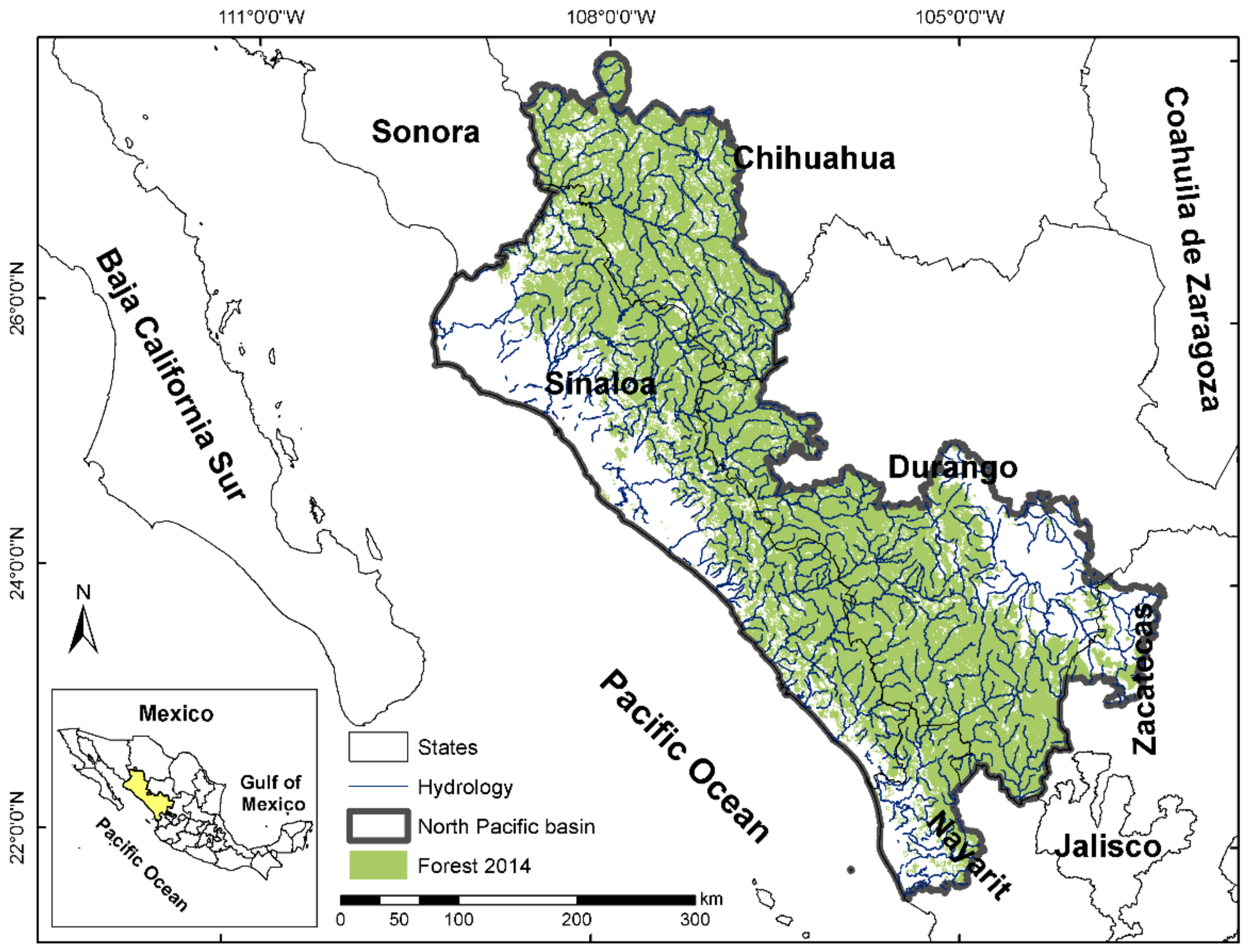
2.1. Study Area

The North Pacific basin is located within the entire state of Sinaloa and also comprises some municipalities of the states of Durango, Chihuahua, Zacatecas and Nayarit in Mexico. The basin has an area of 152,013 km2, of which 64.10% corresponds to forests (primary and secondary coniferous, oak, mountain mesophilic, deciduous, evergreen, sub-deciduous forest, and cultivated forest) (Figure 1). The North Pacific basin represents 8.0% of the surface of Mexico according to the National Institute of Statistics and Geography (INEGI) [45]. The estimated population in the basin is 4,466,000 inhabitants [46]. The population increase and their socioeconomic activities have caused changes in the occupation and land use in some regions of the basin, which have produced the loss of forest cover and therefore negative effects on ecosystems, such as soil degradation, decreases in aquifer storage due to changes in the water cycle and loss of biodiversity, as stated by the National Water Commission (CONAGUA) [47].
As previously described, deforestation has a direct effect in the study area because it is the most fertile valley in Mexico, contributing 30.2% of the cultivated land [48]. Agricultural production is mainly due to the presence of many surface water bodies in this study area, where 13 major rivers and 11 large dams are located throughout the basin and serve different functions, such as water storage, fishing, and irrigation [47].

2.2. Data

Several variables, for example altitude, slope, forest production, restoration areas, soil types, population density, and degraded forest, among others, were considered for the geospatial simulation model (Table 1). The selection of these variables was based on an expert consultation to describe the possible causes of deforestation [49] and was complemented with an extensive bibliographic review [15,31,50,51] and an exhaustive assessment that took into account the availability of information, the objectives of the study and the scenarios to be simulated. Likewise, the official Land-use and vegetation maps of the INEGI at a scale of 1:250,000 were used to perform the analysis of the forest cover [45], and the National Greenhouse Gas Inventory database of Mexico reported by [52].

2.3. Methodology

The geospatial simulation model of deforestation and reforestation was established using the forest cover of 2014 as baseline. The MCE methods were integrated to model deforestation and reforestation of forests. The implementation of MCE techniques began with the definition of the simulation model objectives, as part of the design of the geospatial model. Then, some criteria, factors and restrictions were established for the selection and preprocessing of the data. Finally, the land use demand was calculated and simulation maps for deforestation and reforestation were depicted. The methods and techniques that were used to simulate the geospatial model are described in greater detail in the following section.

2.4. Selection and Preprocessing of Data

First, the official maps of Land-Use and Vegetation (LUV) of the INEGI [45] were used to obtain the analysis of deforestation and reforestation. A geometric and topological correction was applied, and the categories of LUV maps were homogenized according to the Biennial Update Reports (BURs) of the National Greenhouse Gas Inventory of Mexico reported to the United Nations Framework Convention on Climate Change (UNFCCC) [52].
The variables selected for the simulation of the geospatial model were: population density, marginalization index, distance to localities with less than 2500 inhabitants, soil types, distance to roads, distance to hydrographic features, distance to agriculture, distance to grasslands, distance to protected natural areas, forest production, altitude, slope, areas for forest restoration and degraded forests. The variables were spatialized (alphanumeric variables), standardized (legend of classes and uses) and rasterized (vector variables) with a pixel size of 100 m.

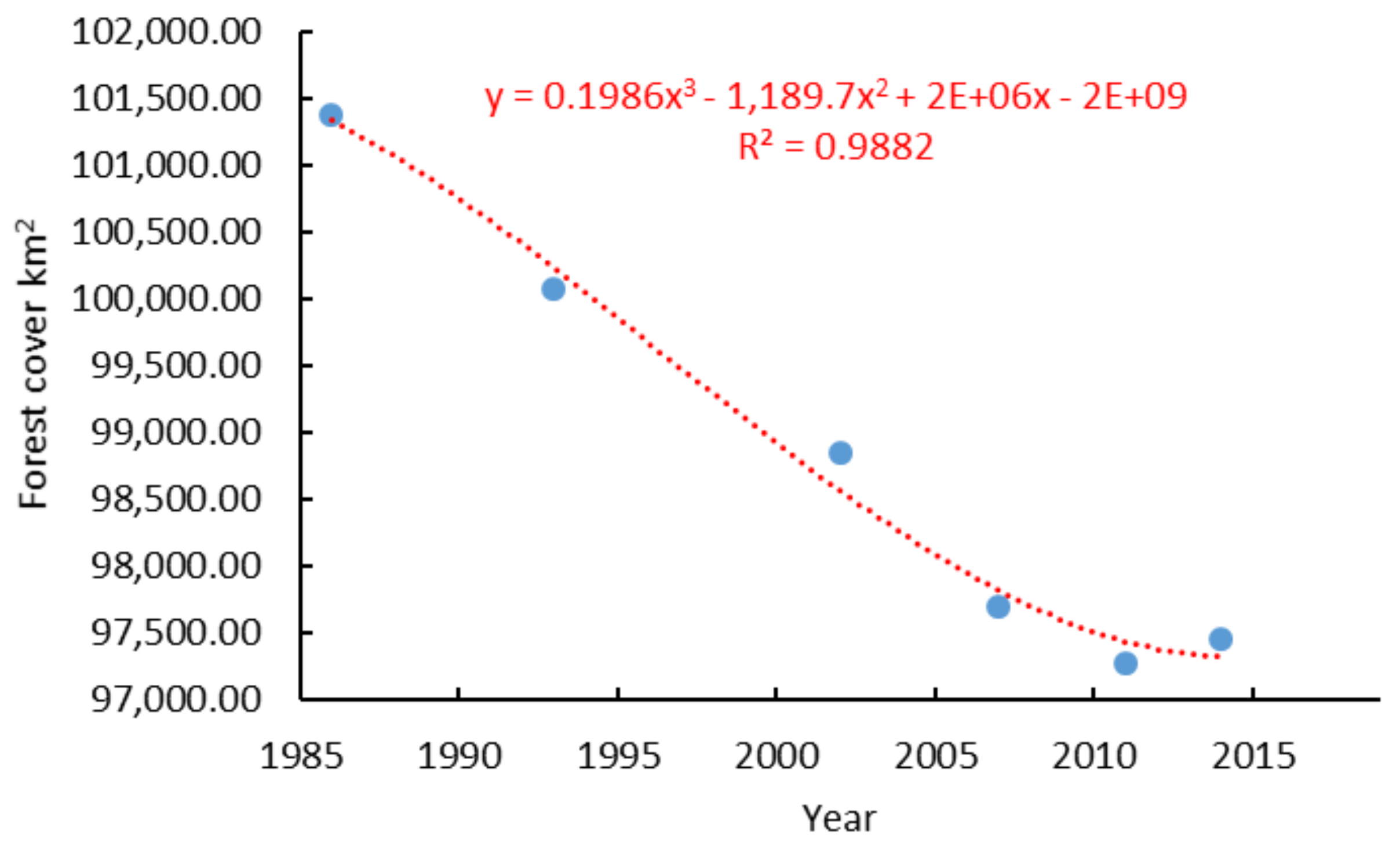
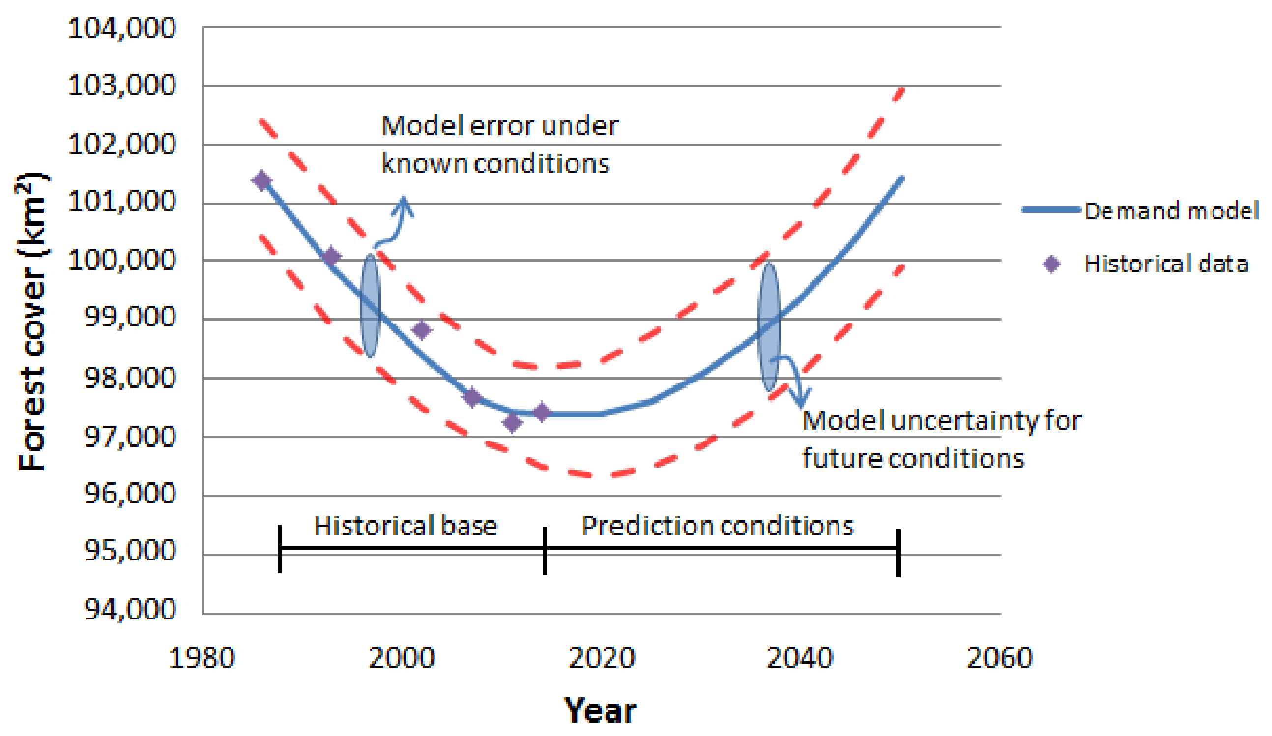
2.5. Demand for Land Use

A land use demand model was developed to simulate the forest area behavior in the future. The Land-use demand simulation consisted of estimating the forest area that would be covered in 2030 and 2050 based on a temporal analysis of the forest areas in 1986, 1993, 2002, 2007, 2011 and 2014 using a third-order polynomial function, of which the precision and uncertainty were analyzed.
Then, the deforestation and reforestation covers for the future scenarios were defined. The annual deforestation and reforestation rates for the future scenarios were established based on the behavior observed for both forest processes in the periods of 1986–1993, 1993–2002, 2002–2007, 2007–2011, and 2011–2014. The deforestation and reforestation scenarios were in accordance with the goals of the National Forest Program of Mexico [53], the Sustainable Forest Development Plan of Mexico [54], and the International Sustainable Development Objectives (SDO) of the Intergovernmental Panel on Climate Change (IPCC) regarding the current and future global state of forests [55], which are aimed to reduce deforestation rates to more than 50% and increase reforestation for 2030 and 2050.

2.6. Geospatial Simulation Using MCE

The Weighted Linear Summation (WLS) was used to obtain the most suitable areas for deforestation and reforestation. The WLS method is based on both weighted factors and constraints [56,57]. Three criteria (biophysical, socioeconomic and proximity) were used. Each criterion was weighted based on external expert opinions and a bibliographic review. The values obtained were later normalized in such a way that the sum of the weights of the three criteria was equal to 1.
Once the criteria were defined and weighted, the variables were modelled according to the objectives of each scenario using land mapping. The biophysical factors (soil types, land use and vegetation, areas for restoration and degraded forests) were characterized by thematic classes. The Saaty analytical hierarchy method was applied with the purpose of establishing a relative hierarchy of importance between the categories of the same factor [58].
The assignment of weights to each thematic class was made considering quantitative and qualitative aspects. From the quantitative point of view, a spatial intersection was made between the variables of deforestation and reforestation during the different periods and the percentage of impact of each class was determined. From the qualitative point of view, the opinions of 8 external experts were used: 3 from the National Forestry Commission (CONAFOR), 3 from the Ministry of the Environment and Natural Resources (SEMARNAT) and 2 from the National Commission of Protected Natural Areas (CONANP). The experts established the weights for the categories of the same factor.
A byte scale of 0–255 was used for factor normalization by using the multi-criteria evaluation module in the TerrSet software. The highest value of the scale represents the highest probability of belonging to the decision group and fuzzy logic techniques were applied according to [59,60]. Table 2 shows the maximum and minimum values observed for each factor. Table 2 also shows the functions and the scale used for the normalization of each factor.
The model restrictions were binary alternatives, where the value of 0 indicated the areas excluded from the analysis and the value of 1 corresponded to the possible locations for simulation. The deforestation model restrictions included all categories of land-use cover, except forest areas where future deforestation is estimated to take place. Regarding the reforestation model, the covers were enabled based on the ability of the areas to be converted into forest areas, such as scrub, pasturelands, areas for restoration, degraded forests, other types of vegetation and other lands.
Once each of the weighted and normalized factors was obtained, the WLS equation (Equation (1)) was used to evaluate the different alternatives. The WLS equation consisted of adding the result of multiplying the individual pixel value of each normalized factor by the final weight assigned to that same factor using the following equation:
r i = j = 1 n w j v i j
where r i is the adequacy level of alternative i , w i is the weight of factor j , and v i j is the weighted value of alternative i of factor j .
Since future conditions can differ from the historical data, an uncertainty analysis was carried out to describe the range of potential forest cover in the North Pacific Basin at the 95% confidence level. Besides, the Extended Fourier Amplitude Sensitivity Test (E-FAST) technique suggested by [61] was used to determine the stability/robustness of the model results through the first order sensitivity indices ( S i ) . The E-FAST technique is based on variance estimation and uses a Monte Carlo simulation for generating random samples (probability distributions) for each of the independent input factors used in the geospatial model [62]. The E-FAST test did not require any particular assumptions on the model structure, and provided quantitative sensitivity measures for each factor. The first order sensitivity indices ( S i ) measured how the i th factor contributes to the variation of the model results without taking into account the interactions with other input parameters. A detailed description of the E-FAST method is given in [61].
The sensitivity analysis using the E-FAST technique was implemented according to the following procedure: first, the frequency distribution of the factors was established; then, a sample of the different factors used in the model was extracted. The sensitivity analysis consisted in fluctuating each of the input factors. Each of the model factors’ values were decreased and increased by 25%, while the others were steady. The model was executed 5100 times. The forest cover deviations were used to calculate sensitivity indices and reflected the model sensitivity. Finally, the sensitivity indices ( S i ) were obtained and analyzed.
Once the uncertainty and robustness of the geospatial simulation model was evaluated, the suitability maps (deforestation and reforestation maps) were obtained from the geospatial simulation model. Then, a multiobjective assignment (MOLA: multiobjective land allocation) was carried out with the assumption that the deforestation and reforestation covers are conflicted and interacted with each other [63].

2.7. Indicators and Mapping of Carbon Loss and Capture

An intersection between the land-use and vegetation (LUV) map of the baseline year (2014) and the map obtained from the geospatial simulation model was used to determine the indicators of change and sustainability for the simulated deforestation and reforestation processes. The carbon balance was estimated based on the carbon loss by deforestation and carbon capture by reforestation. The carbon balance is related to live aerial biomass and roots and is expressed in tons of Carbon (ton/C), as indicated in the National Greenhouse Gas Inventory in Mexico reported by [52]. Therefore, the distribution maps of carbon loss and capture were obtained for the 2014–2030 and 2014–2050 periods.

3. Results

3.1. Land Use Demand

The analysis of deforestation and reforestation in the study area is presented for during the period of 1986–1993, 1993–2002, 2002–2007, 2007–2011 and 2011–2014 (Figure 2). A dramatic decrease in forest cover during the period of 1986–2007 is evidenced due to deforestation in the North Pacific basin (Figure 2a). However, the reforestation process was slightly superior to the deforestation process at the end of the study period during 2011–2014 (Figure 2b).
Two different ways of reforestation can be recognized in the study area: natural forest regeneration and forestry plantations. However, no differentiation between both processes can be completely identified since only 100 ha are related to forest plantations, according to official information provided by INEGI [45]. Based on deforestation and reforestation analysis, a demand model for the land area covered by forests was developed (Figure 3).
The land demand model obtained is a simplification of the real forest cover behavior observed in the North Pacific Basin. The assumptions, input data and other criteria used for the model development are representative of the real conditions and they can be inaccurate. Therefore, measuring the precision with which the demand model can reproduce observed conditions is very important since the usefulness of the model depends on its accuracy and reliability. In the present study, the forest cover time series was adjusted to a 3rd order polynomial function. The equation of the fitted model is
y = 0.1986 x 3 1189.7 x 2 + 2,375,098.7 x 1,580,264,028.01
The third order polynomial model observed a reliability of 98.8%, which could be considered as a good fit (Table 3). The performance of the land demand model in fitting the historical data was also assessed by using the standard error of the estimate S E and the mean absolute error M A E . The standard error of the estimate shows that the standard deviation of the residuals is 279.968. This value was used to construct prediction limits for future observations. The M A E of 173.272 represents the average value of the residuals.
Since future conditions can differ from the historical data, an uncertainty analysis was carried out to describe the range of potential forest cover in the North Pacific Basin at the 95% confidence level (Figure 4). The range of uncertainty is related to a frequency distribution that characterizes the variability of deforestation and reforestation in the study area. The variability observed under future scenarios can be related to inadequate information, incorrect assumptions and the natural variability of forest processes (in particular, natural variation related to reforestation).
According to model results, a forest cover of 98,713.52 km2 was estimated for 2030, while a value of 101,239.8 km2 was estimated for 2050. The deforestation and reforestation areas and their mean annual values for 2030 and 2050 were determined in Table 4.
The results show that the forest cover estimated for 2050 was similar to that observed in 1986. The forest cover recovery estimated for 2050 can be explained by the annual averages of reforestation expected for the 2014–2030 and 2030–2050 periods, which were greater than the annual average deforestation projected.

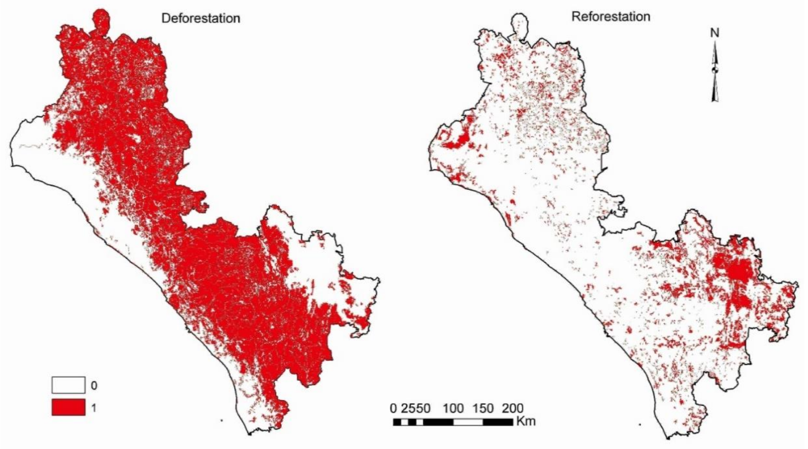
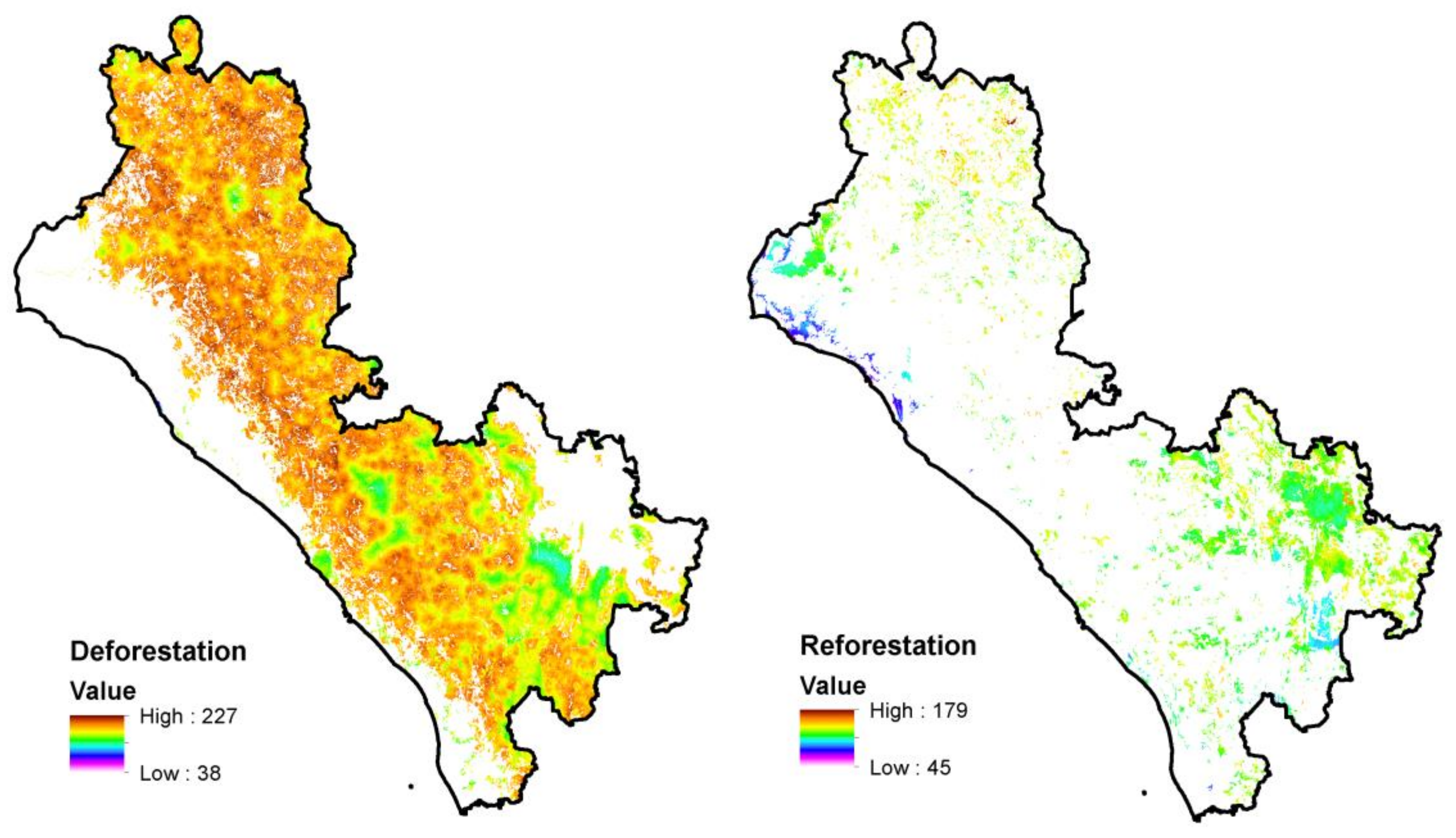
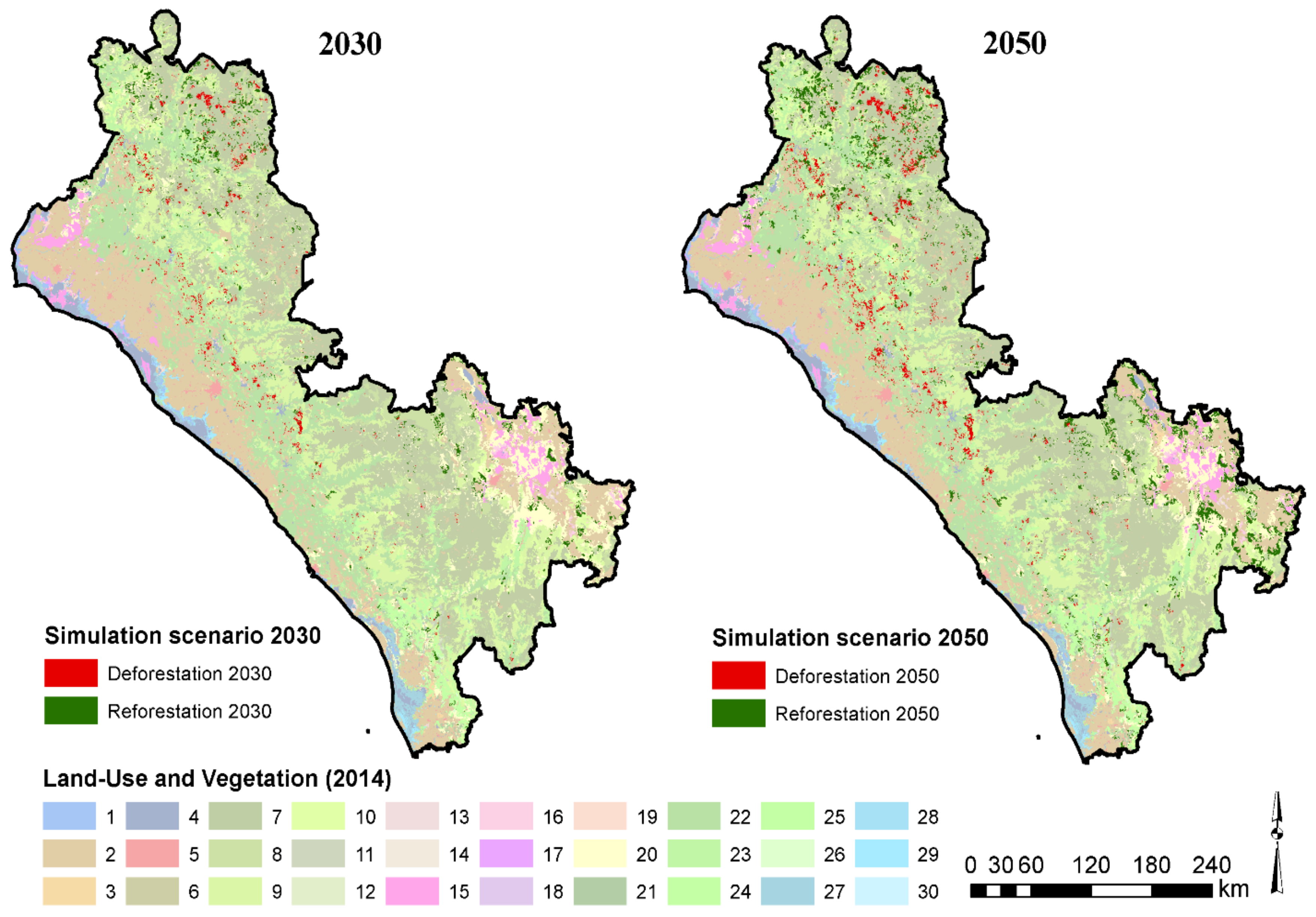
3.2. Geospatial Simulation Using MCE

The weighting criteria results and the factors assigned by the consulting experts and the bibliographic reviews are summarized in Table 5. The weighting criteria (Wc), the weighting factors (Wi), and the final weights assigned to the factors (Wj) are identified.
Table 6 shows the weighting results by the categorical factors: soil types, land use and vegetation, degraded forests and areas for restoration. The categorical factors results were obtained using the Saaty pairwise comparison method, and their importance was assigned to each class according to the opinion of experts, resulting in a consistency coefficient (c).
Through fuzzy logic techniques, 16 normalized factors were obtained with a scale from 0 to 255 (Figure 5). It should be noted that the Land-use and vegetation factor was normalized twice, depending on the objective to be simulated (deforestation and reforestation). Additionally, all other factors were only normalized once for both simulation objectives.
The model restrictions for deforestation and reforestation were depicted, respectively (Figure 6). For the deforestation objective, only the forest categories were activated, while for the reforestation, the categories of scrub, pasturelands, areas for restoration, degraded forests, other types of vegetation and other lands were activated.
Once all normalized factors, restrictions and weights were obtained, the WLS equation was applied to generate suitability maps for deforestation and reforestation (Figure 7).
According to the results obtained from E-FAST, the factors with the highest weights were considered as the most sensitive factors in the model (Table 7). Any change in any of the most sensitive factors represents a significant impact on the model. The most important factor was Forest Production for both objectives (deforestation and reforestation) with a S i of 0.236 and 0.416, respectively. For the deforestation objective, other factors with greater importance were the Marginalization Index, Distance to Protected Natural Areas, Slope, and Distance to Agriculture with S i indices of 0.114, 0.102, 0.093 and 0.079, respectively. For the reforestation objective, the most sensitive factors were the Slope and Altitude with S i values of 0.183 and 0.073, respectively, followed by the Distance to Agriculture ( S i = 0.059) and Soil Types ( S i = 0.046).
Afterwards, a classification (ranking) of each of the resulting objectives (suitability maps) was carried out, and a multiobjective allocation was made to solve possible conflicts. Thus, the scenarios proposed for 2030 and 2050 were obtained according to the required land demand for each objective (Figure 8).

3.3. Indicators and Mapping of Carbon Loss and Capture

To analyze the future perspectives of the model, an impact analysis of the land use and vegetation in the basin was carried out. According to the forecast results, deforestation by 2030 would occur mainly in areas of primary deciduous forest (33.60%), primary coniferous forest (31.87%), secondary deciduous forest (13.85%) and primary oak forest (10.37%); meanwhile, reforestation in 2030 would take place on grasslands (86.77%) and degraded forests (11.64%) (Figure 9).
Regarding the 2050 scenario, the deforestation model indicated that the most impacted categories would be primary deciduous forest, primary coniferous forest, secondary deciduous forest and primary oak forest, with deforested area percentages of 36.35%, 29.35%, 14.00% and 10.73%, respectively, regarding the total deforested area expected. The reforestation in 2050 would be concentrated in the grasslands and degraded forest categories, with 83.85% and 13.67%, respectively (Figure 8).
Subsequently, the indicators of carbon capture and loss in live aerial biomass and roots were estimated with respect to the deforested and reforested covers of the proposed scenarios. For the 2014–2030 period, 105,428.04 ton/C would be lost due to deforestation, while 121,637.71 ton/C would be captured by reforestation. During the 2030–2050 period, it was estimated that 109,242.02 ton/C could be lost, while 696,838.03 ton/C could be captured (Table 8). The carbon capture and loss scenarios indicate a forest cover recovery in the study area, with a positive impact from the environmental point of view. The results obtained are promising in terms of climate change mitigation at local and regional level.
Finally, the carbon loss and capture distribution maps were generated, which in turn were referred to the geospatial simulation model of 2030 and 2050. The spatial distribution of the carbon loss by deforestation in the different categories was depicted in the same way as the carbon capture by reforestation (Figure 9).

4. Discussion

The results showed that the present study contributed significantly to the management of forest ecosystems and to decision-making processes by providing information on the future state of forest cover in North Pacific Basin in Mexico.
First, a novel procedure is proposed to estimate the land use demand for the forest cover, by combining a retrospective analysis (time series analysis) and a non-linear regression (3rd order polynomial function) to describe the forest cover behavior towards the years 2030 and 2050. Based on a historical analysis of deforestation and reforestation in the study area, the average annual rates of both forest processes were estimated. This procedure can be considered novel because other simulations usually only use the land use tendency, such as Markov chains [64] and cellular automata [65].
The proposed model could be considered as a sustainable alternative for all the stakeholders and decision-makers in government since future deforestation is proposed on degraded forest areas, which will not affect forests with high environmental importance. Likewise, the expected reforestation showed a positive impact in terms of mitigating the emission of greenhouse gases in the basin.
Most of studies in the literature have focused on a single objective, such as developing deforestation scenarios [26,36,37,38,66], and few studies have included the reforestation [39,40]. However, no studies were found that consider both forest processes at the same time to generate the future simulation of the forest cover, since conflicts arise when determining whether an area can be deforested or reforested in the future.
Besides which, the proposed model includes variables, such as forest production, degraded forests, and areas for restoration, that have not been included in other studies to determine the most suitable areas for deforestation or reforestation. The weighting criteria and the weights assigned to categorical variables also differ from other studies that have used MCE [32,67,68]. The weights of categorical variables were assigned from two points of view: the qualitative criteria, which was based on the opinion of experts and the quantitative criteria, which considered spatial computations.
Sometimes, the forest classification information provided by official sources can be ambiguous. For instance, an in-depth classification of the mountain forests in the study area can be found in [69], which differs from the classification provided by INEGI [45]. Therefore, the development of geospatial models must be supported with a highly detailed classification of forests (such as biogeographic or ecologic classification), which could be of interest for other specialists.
Natural regeneration of the forest is a normal induced ecological phenomenon of succession, while forest plantation (especially with non-native species) is an ecologically undesirable practice [70,71,72]. Differentiating the natural reforestation process from the induced planting process is a common problem in geosimulation that could be solved using very high resolution data (spatial, spectral and radiometric) derived from remote sensors [73,74]. Therefore, a more in-depth information from an ecological point of view could be obtained through the remote sensing analysis of high resolution data.
The geospatial model estimated the carbon loss and capture by deforestation and reforestation processes. As a result, distribution maps of the carbon loss and capture for 2030 and 2050 were obtained, generating indicators to support the decision-making process for forest management, mitigation and planning purposes, which are directly related to climate change at the local, regional and global levels. Given that some studies suggest that carbon storage comes directly from forest cover [75,76], the present study can also help to visualize future distribution of ecosystem services.
Finally, the proposed methodological approach for the implementation of the scenarios could be useful for generating other ecological indicators and can be applied to other basins considered as a priority by the institutions involved in forest planning and management.

5. Conclusions

The geospatial simulation model provides relevant information on a possible future state of the forest cover in North Pacific basin. Based on the scenarios simulated for 2050, the forest cover in the study area would be similar to the observed in in 1986, which would be fulfilling the National Forest Program goals.
The suitability areas of deforestation and reforestation were estimated and mapped. This simulation showed a decrease in the mean annual rates of deforestation, where mean annual rates of 115 km2 and 95 km2 are expected for the 2014–2030 and 2030–2050 periods. During the same period, an increase in the mean annual reforestation rates was identified, with mean annual rates of 193.84 km2 and 221.31 km2, respectively. The sensitivity analysis using E-FAST identified the most significant factors in the deforestation and reforestation models. In particular, the Biophysical factors were recognized as the most important parameters of the model.
Based on the results obtained in the present study, the geospatial simulation model showed sustainable simulation scenarios from a forest management point of view. The model uncertainty analysis showed that even in the worst case scenario, the North Pacific basin shows a recovery in forest cover by 2050. The loss and carbon capture were estimated and mapped, considering the forest cover predicted by the deforestation and reforestation model. A carbon capture of 16,209.67 ton/C was estimated for the 2014–2030 period and 587,596.01 ton/C for the 2030–2050 period. The most affected land use categories were the primary deciduous forest, primary coniferous forest and secondary deciduous forest. In contrast, grassland and degraded forest categories were identified as the most suitable covers for reforestation. This information is of a great importance for government institutions for the management and planning of forest ecosystems.
The present study demonstrated that the geospatial analysis techniques and multicriteria evaluation are viable strategies for the development of forest management scenarios, since they take into account different perspectives such as the experts’ opinions, national and international goals, and a set of biophysical, socioeconomic and proximity variables that generated a robust methodology that can be used to predict deforestation and reforestation processes in different regions around the world.

Author Contributions

Conceptualization, S.A.M.-A. and W.P.-R.; methodology, S.A.M.-A., C.E.P.-A. and W.P.-R.; formal analysis, S.A.M.-A., C.F.-O. and J.G.R.-P.; investigation, S.A.M.-A. and C.E.P.-A.; writing—original draft preparation, S.A.M.-A.; writing—review and editing, S.A.M.-A., W.P.-R., J.G.R.-P. and C.F.-O. All authors have read and agreed to the published version of the manuscript.

Funding

This research received no external funding.

Acknowledgments

Thanks to the Faculty of Earth and Space Sciences and the Autonomous University of Sinaloa.

Conflicts of Interest

The authors declare no conflict of interest.

References

  1. Swedan, N. Deforestation and land farming as regulators of population size and climate. Acta Ecol. Sin. 2020, 40, 443–450. [Google Scholar] [CrossRef]
  2. Buizer, M.; Humphreys, D.; De Jong, W. Climate change and deforestation: The evolution of an intersecting policy domain. Environ. Sci. Policy 2014, 35, 1–11. [Google Scholar] [CrossRef] [Green Version]
  3. Sekhran, N.; Bovarnick, A.; Scott, T.; Corcoran, J. Biodiversity, Development and Poverty Alleviation. 2010. Available online: https://www.cbd.int/doc/bioday/2010/idb-2010-booklet-en.pdf (accessed on 10 December 2020).
  4. FAO. Global Forest Resources Assessment 2020 Key Findings. Available online: http://www.fao.org/3/CA8753EN/CA8753EN.pdf (accessed on 23 June 2020).
  5. Panday, P.K.; Coe, M.T.; Macedo, M.N.; Lefebvre, P.; Castanho, A.D.A. Deforestation offsets water balance changes due to climate variability in the Xingu River in eastern Amazonia. J. Hydrol. 2015, 523, 822–829. [Google Scholar] [CrossRef]
  6. Houghton, R. Carbon emissions and the drivers of deforestation and forest degradation in the tropics. Curr. Opin. Environ. Sustain. 2012, 4, 597–603. [Google Scholar] [CrossRef]
  7. Gao, J.; Gao, H.; Zhou, C.; Zhang, X. The impact of land-use change on water-related ecosystem services: A study of the Guishui River Basin, Beijing, China. J. Clean. Prod. 2017, 163, S148–S155. [Google Scholar] [CrossRef]
  8. Mohebalian, P.M.; Aguilar, F.X. Design of tropical forest conservation contracts considering risk of deforestation. Land Use Policy 2018, 70, 451–462. [Google Scholar] [CrossRef]
  9. Gingrich, S.; Lauk, C.; Niedertscheider, M.; Pichler, M.; Schaffartzik, A.; Schmid, M.; Mager, A.; Noë, J.; Bhan, M.; Erb, K. Hidden emissions of forest transitions: A socio-ecological reading of forest change. Curr. Opin. Environ. Sustain. 2019, 38, 14–21. [Google Scholar] [CrossRef]
  10. Moomaw, W.R.; Law, B.E.; Goetz, S.J. Focus on the role of forests and soils in meeting climate change mitigation goals: Summary. Environ. Res. Lett. 2020, 15, 1–9. [Google Scholar] [CrossRef]
  11. Dooley, K.; Kartha, S. Land-based negative emissions: Risks for climate mitigation and impacts on sustainable development. Int. Environ. Agreem. 2018, 18, 79–98. [Google Scholar] [CrossRef]
  12. Singh, S.; Reddy, C.S.; Pasha, S.V.; Dutta, K.; Saranya, K.R.L.; Satish, K.V. Modeling the spatial dynamics of deforestation and fragmentation using Multi-Layer Perceptron neural network and landscape fragmentation tool. Ecol. Eng. 2017, 99, 543–551. [Google Scholar] [CrossRef]
  13. Overmars, K.P.; Verburg, P.H. Multilevel modelling of land use from field to village level in the Philippines. Agric. Syst. 2006, 89, 435–456. [Google Scholar] [CrossRef]
  14. Verburg, P.H.; Overmars, K.P.; Huigen, M.G.A.; de Groot, W.T.; Veldkamp, A. Analysis of the effects of land use change on protected areas in the Philippines. Appl. Geogr. 2006, 26, 153–173. [Google Scholar] [CrossRef]
  15. Bax, V.; Francesconi, W.; Quintero, M. Spatial modeling of deforestation processes in the Central Peruvian Amazon. J. Nat. Conserv. 2016, 29, 79–88. [Google Scholar] [CrossRef]
  16. De Barros Ferraz, S.F.; Vettorazzi, C.A.; Theobald, D.M.; Ballester, M.V.R. Landscape dynamics of Amazonian deforestation between 1984 and 2002 in central Rondônia, Brazil: Assessment and future scenarios. For. Ecol. Manag. 2005, 204, 69–85. [Google Scholar] [CrossRef]
  17. Hurtado Pidal, J.R. Analysis, Modeling and Spatial Simulation of the Land Cover Change, between Natural Areas and Those of Anthropic Origin in the Province of Napo (Ecuador), for the Period 1990–2020. Master’s Thesis, Universidad Nacional de La Plata, Buenos Aires, Argentina, 2014. [Google Scholar]
  18. Rodríguez-Eraso, N. Land-Cover and Land-Use Change and Deforestation in Colombia: Spatial Dynamics, Drivers and Modelling. Ph.D. Thesis, Universitat Autònoma de Barcelona, Barcelona, Spain, 2011. [Google Scholar]
  19. Gibon, A.; Sheeren, D.; Monteil, C.; Ladet, S.; Balent, G. Modelling and simulating change in reforesting mountain landscapes using a social-ecological framework. Landsc. Ecol. 2010, 25, 267–285. [Google Scholar] [CrossRef] [Green Version]
  20. An, L.; Linderman, M.; Qi, J.; Shortridge, A.; Liu, J. Exploring complexity in a human-environment system: An agent-based spatial model for multidisciplinary and multiscale integration. Ann. Assoc. Am. Geogr. 2005, 95, 54–79. [Google Scholar] [CrossRef]
  21. Matthews, R.B.; Gilbert, N.G.; Roach, A.; Polhill, J.G.; Gotts, N.M. Agent-based land-use models: A review of applications. Landsc. Ecol. 2007, 22, 1447–1459. [Google Scholar] [CrossRef] [Green Version]
  22. Moreno, N.; Quintero, R.; Ablan, M.; Barros, R.; Dávila, J.; Ramírez, H.; Tonella, G.; Acevedo, M.F. Biocomplexity of deforestation in the Caparo tropical forest reserve in Venezuela: An integrated multi-agent and cellular automata model. Environ. Model. Softw. 2007, 22, 664–673. [Google Scholar] [CrossRef]
  23. Babbar, D.; Areendran, G.; Sahana, M.; Sarma, K.; Raj, K.; Sivadas, A. Assessment and prediction of carbon sequestration using Markov chain and InVEST model in Sariska Tiger Reserve, India. J. Clean. Prod. 2021, 278, 123333. [Google Scholar] [CrossRef]
  24. Franco Prieto, C.A. Development of a Model Based on Multicriteria Spatial Analysis for the Determination of Forest Management Units. Case of the Department of Casanare. Master’s Thesis, Universidad Nacional de Colombia, Bogota, Colombia, 2011. [Google Scholar]
  25. Maestripieri, N.; Houet, T.; Paegelow, M.; Selleron, G.; Toro Balbontín, D.; Sáez Villalobos, N. Dynamic simulation of forest management normative scenarios: The case of timber plantations in the southern Chile. Futures 2017, 87, 65–77. [Google Scholar] [CrossRef]
  26. Silva, A.C.O.; Fonseca, L.M.G.; Körting, T.S.; Escada, M.I.S. A spatio-temporal Bayesian Network approach for deforestation prediction in an Amazon rainforest expansion frontier. Spat. Stat. 2020, 35, 100393. [Google Scholar] [CrossRef]
  27. Jiang, Q.; Cheng, Y.; Jin, Q.; Deng, X.; Qi, Y. Simulation of Forestland Dynamics in a Typical Deforestation and Afforestation Area under Climate Scenarios. Energies 2015, 8, 10558–10583. [Google Scholar] [CrossRef]
  28. Zupko, R.; Rouleau, M. ForestSim: Spatially explicit agent-based modeling of non-industrial forest owner policies. SoftwareX 2019, 9, 117–125. [Google Scholar] [CrossRef]
  29. Zambelli, P.; Lora, C.; Spinelli, R.; Tattoni, C.; Vitti, A.; Zatelli, P.; Ciolli, M. A GIS decision support system for regional forest management to assess biomass availability for renewable energy production. Environ. Model. Softw. 2012, 38, 203–213. [Google Scholar] [CrossRef]
  30. Thapa, R.B.; Shimada, M.; Watanabe, M.; Motohka, T.; Shiraishi, T. L-band SAR data and spatially explicit model to analyse forest loss between 2007 and 2030 in central Sumatra. In Proceedings of the 2013 Asia-Pacific Conference on Synthetic Aperture Radar (APSAR), Tsukuba, Japen, 23–27 September 2013; pp. 108–111. [Google Scholar]
  31. Mas, F.-J.; Sorani, V.; Alvarez, R. Elaboración de un Modelo de Simulación del Proceso de Deforestación. Investig. Geogr. 1996, 43–57. Available online: https://www.redalyc.org/pdf/569/56909907.pdf (accessed on 21 January 2019).
  32. Jaimes, N.B.P.; Sendra, J.B.; Delgado, M.G.; Plata, R.F.; Némiga, X.A.; Solís, L.R.M. Determination of Optimal Zones for Forest Plantations in the State of Mexico Using Multi-Criteria Spatial Analysis and GIS. J. Geogr. Inf. Syst. 2012, 4, 204–218. [Google Scholar] [CrossRef] [Green Version]
  33. Sahagún-Sánchez, F.J.; Reyes-Hernández, H.; Flores, J.L.F.; Vargas, L.C. Modeling of scenarios of potential change in vegetation and land use in the Sierra Madre Oriental de San Luis Potosí, Mexico. J. Lat. Am. Geogr. 2011, 10, 65–86. [Google Scholar] [CrossRef]
  34. Mas, J.-F.; Flamenco, A. Modeling of Land Cover/Use Changes in a Tropical Region of Mexico. Available online: http://www.geotropico.org/NS_5_1_Mas-Flamenco.pdf (accessed on 21 January 2019).
  35. Leija-Loredo, E.; Reyes-Hernandez, H.; Reyes-Perez, O.; Flores-Flores, J.; Sahagún-Sanchéz, F. Changes in vegetation cover, land uses and future scenarios in the coastal region of the state of Oaxaca, Mexico. Madera y Bosques 2016, 22, 125–140. [Google Scholar]
  36. Piontekowski, V.J.; Ribeiro, F.P.; Matricardi, E.A.T.; Lustosa, I.M.; Bussinguer, A.P.; Gatto, A. Modeling deforestation in the state of Rondonia. Floresta e Ambiente 2019, 26, 20180441. [Google Scholar] [CrossRef] [Green Version]
  37. Ayele, G.; Hayicho, H.; Alemu, M. Land Use Land Cover Change Detection and Deforestation Modeling: In Delomena District of Bale Zone, Ethiopia. J. Environ. Prot. 2019, 10, 532–561. [Google Scholar] [CrossRef] [Green Version]
  38. Naffaa, S.; van Beek, L.P.H.; Dunn, F.E.; de Jong, S. Modeling the changing sediment yield of the Amazon under climate change and deforestation scenarios and the possible impacts on the Guiana coast. In Proceedings of the 22nd EGU General Assembly (EGUGA 2020), Online, 4–8 May 2020; p. 18621. [Google Scholar]
  39. Lochhead, K.; Ghafghazi, S.; LeMay, V.; Bull, G.Q. Examining the vulnerability of localized reforestation strategies to climate change at a macroscale. J. Environ. Manag. 2019, 252, 109625. [Google Scholar] [CrossRef] [PubMed]
  40. Lieffers, V.J.; Pinno, B.D.; Beverly, J.L.; Thomas, B.R.; Nock, C. Reforestation policy has constrained options for managing risks on public forests. Can. J. For. Res. 2020, 50, 855–861. [Google Scholar] [CrossRef]
  41. Manson, S.M. Agent-based modeling and genetic programming for modeling land change in the Southern Yucatán Peninsular Region of Mexico. Agric. Ecosyst. Environ. 2005, 111, 47–62. [Google Scholar] [CrossRef]
  42. House, J.I.; Colin Prentice, I.; Le Quéré, C. Maximum impacts of future reforestation or deforestation on atmospheric CO2. Glob. Chang. Biol. 2002, 8, 1047–1052. [Google Scholar] [CrossRef]
  43. Nakicenovic, N.; Alcamo, J.; Davis, G.; de Vries, B. Emissions Scenarios; Cambridge University Press: Cambridge, UK, 2000. [Google Scholar]
  44. Veldkamp, E.; Schmidt, M.; Powers, J.S.; Al, E. Deforestation and reforestation impacts on soils in the tropics. Nat. Rev. Earth Environ. 2020, 1, 590–605. [Google Scholar] [CrossRef]
  45. INEGI. Uso de Suelo y Vegetación. Available online: http://www.beta.inegi.org.mx/temas/mapas/usosuelo/ (accessed on 27 August 2019).
  46. INEGI. Encuesta Intercensal 2015. Available online: http://www.beta.inegi.org.mx/proyectos/enchogares/especiales/intercensal/ (accessed on 27 August 2019).
  47. CONAGUA, C.N. del A. Programa Hídrico Regional Visión 2030. Región Hidrológico-Administrativa III Pacífico Norte. Available online: http://www.conagua.gob.mx/conagua07/publicaciones/publicaciones/3-sgp-17-12pn.pdf (accessed on 27 August 2019).
  48. CONAGUA, C.N. del A. Estadísticas Agrícolas de los Distritos de Riego Año agrícola 2013–2014. Available online: https://bpo.sep.gob.mx/#/recurso/615 (accessed on 27 August 2019).
  49. Monjardín-Armenta, S.A.; Pacheco-Angulo, C.E.; Plata-Rocha, W.; Corrales-Barraza, G. Deforestation and its causal factors in the state of Sinaloa, Mexico. Madera Bosques 2017, 23, 7. [Google Scholar] [CrossRef] [Green Version]
  50. Osorio, L.P.; Mas, J.-F.; Guerra, F.; Maass, M. Analysis and modeling of deforestation processes: A case study in the Coyuquilla River Basin, Guerrero, Mexico. Investig. Geogr. 2015, 88, 60–74. [Google Scholar] [CrossRef] [Green Version]
  51. Pineda Jaimes, N.B.; Bosque Sendra, J.; Gómez Delgado, M.; Franco Plata, R. Exploring the driving forces behind deforestation in the state of Mexico (Mexico) using geographically weighted regression. Appl. Geogr. 2010, 30, 576–591. [Google Scholar] [CrossRef]
  52. INECC; CONAFOR. First Biennial Update Report to the United Nations Framework Convention on Climate Change Executive Summary. Available online: https://unfccc.int/sites/default/files/resource/ExecutiveSummary_1.pdf (accessed on 21 November 2019).
  53. SEGOB. Programa Nacional Forestal 2014–2018. Available online: http://dof.gob.mx/nota_detalle.php?codigo=5342498&fecha=28/04/2014 (accessed on 14 February 2019).
  54. CONAFOR. Estrategia Nacional para REDD+. Available online: http://www.conafor.gob.mx:8080/documentos/docs/35/5559ElementosparaeldiseñodelaEstrategiaNacionalparaREDD_.pdf (accessed on 26 February 2019).
  55. FAO. The State of the World’s Forests Forests and Agriculture: Challenges and Opportunities. Available online: http://www.fao.org/3/a-i5850s.pdf (accessed on 26 February 2019).
  56. Li, H.; Ma, Z.; Zhu, Y.; Liu, Y.; Yang, X. Planning and prioritizing forest landscape restoration within megacities using the ordered weighted averaging operator. Ecol. Indic. 2020, 116, 106499. [Google Scholar] [CrossRef]
  57. Irina, L.T.; Javier, B.P.; Teresa, C.B.M.; Eurídice, L.A.; Luz María del Carmen, C.I. Integrating ecological and socioeconomic criteria in a GIS-based multicriteria-multiobjective analysis to develop sustainable harvesting strategies for Mexican oregano Lippia graveolens Kunth, a non-timber forest product. Land Use Policy 2019, 81, 668–679. [Google Scholar] [CrossRef]
  58. Saaty, T. The Analytic Hierarchy Process: Planning, Priority Setting, Resource Allocation; McGraw-Hill International Book Co.: New York, NY, USA; London, UK, 1980; ISBN 0070543712. [Google Scholar]
  59. Aydi, A. Evaluation of groundwater vulnerability to pollution using a GIS-based multi-criteria decision analysis. Groundw. Sustain. Dev. 2018, 7, 204–211. [Google Scholar] [CrossRef]
  60. Azareh, A.; Rafiei Sardooi, E.; Choubin, B.; Barkhori, S.; Shahdadi, A.; Adamowski, J.; Shamshirband, S. Incorporating multi-criteria decision-making and fuzzy-value functions for flood susceptibility assessment. Geocarto Int. 2019, 1–21. [Google Scholar] [CrossRef]
  61. Saltelli, A.; Tarantola, S.; Chan, K.P.S. A quantitative model-independent method for global sensitivity analysis of model output. Technometrics 1999, 41, 39–56. [Google Scholar] [CrossRef]
  62. Brunetti, G.; Šimůnek, J.; Turco, M.; Piro, P. On the use of global sensitivity analysis for the numerical analysis of permeable pavements. Urban Water J. 2018, 15, 269–275. [Google Scholar] [CrossRef] [Green Version]
  63. Lahiji, R.N.; Dinan, N.M.; Liaghati, H.; Ghaffarzadeh, H.; Vafaeinejad, A. Scenario-based estimation of catchment carbon storage: Linking multi-objective land allocation with InVEST model in a mixed agriculture-forest landscape. Front. Earth Sci. 2020. [Google Scholar] [CrossRef]
  64. Verburg, P.H.; Alexander, P.; Evans, T.; Magliocca, N.R.; Malek, Z.; Rounsevell, M.D.A.; van Vliet, J. Beyond land cover change: Towards a new generation of land use models. Curr. Opin. Environ. Sustain. 2019, 38, 77–85. [Google Scholar] [CrossRef]
  65. Roodposhti, M.S.; Aryal, J.; Bryan, B.A. A novel algorithm for calculating transition potential in cellular automata models of land-use/cover change. Environ. Model. Softw. 2019, 112, 70–81. [Google Scholar] [CrossRef]
  66. Stan, K.; Sanchez-Azofeifa, A. Deforestation and secondary growth in Costa Rica along the path of development. Reg. Environ. Chang. 2019, 19, 587–597. [Google Scholar] [CrossRef]
  67. Gracelli, R.R.; Magalhaes, I.B.; Santos, V.J.; Calijuri, M.L. Effects on Streamflow Caused by Reforestation and Deforestation in A Brazilian Southeast Basin: Evaluation by Multicriteria Analysis and Swat Model. In Proceedings of the 2020 IEEE Latin American GRSS and ISPRS Remote Sensing Conference (LAGIRS 2020), Santiago, Chile, 22–26 March 2020; pp. 167–172. [Google Scholar]
  68. Follador, M.; Villa, N.; Paegelow, M.; Renno, F.; Bruno, R. Tropical deforestation modelling: Comparative analysis of different predictive approaches. The case study of Peten, Guatemala. Environ. Sci. Eng. 2008, 77–107. [Google Scholar] [CrossRef] [Green Version]
  69. González-Elizon, M.S.; González-Elizondo, M.; Tena-Flores, J.A.; Ruacho-González, L.; López-Enríquez, I.L. Vegetation of the Sierra Madre Occidental, Mexico: A synthesis. Acta Bot. Mex. 2012, 100, 351–403. [Google Scholar] [CrossRef] [Green Version]
  70. Dyderski, M.K.; Jagodziński, A.M. Drivers of invasive tree and shrub natural regeneration in temperate forests. Biol. Invasions 2018, 20, 2363–2379. [Google Scholar] [CrossRef] [Green Version]
  71. Stanturf, J.A.; Palik, B.J.; Dumroese, R.K. Contemporary forest restoration: A review emphasizing function. For. Ecol. Manag. 2014, 331, 292–323. [Google Scholar] [CrossRef]
  72. Dey, D.C.; Knapp, B.O.; Battaglia, M.A.; Deal, R.L.; Hart, J.L.; O’Hara, K.L.; Schweitzer, C.J.; Schuler, T.M. Barriers to natural regeneration in temperate forests across the USA. New For. 2019, 50, 11–40. [Google Scholar] [CrossRef]
  73. Gerlein-Safdi, C.; Keppel-Aleks, G.; Wang, F.; Frolking, S.; Mauzerall, D.L. Satellite Monitoring of Natural Reforestation Efforts in China’s Drylands. One Earth 2020, 2, 98–108. [Google Scholar] [CrossRef] [Green Version]
  74. Almeida, D.R.A.; Stark, S.C.; Chazdon, R.; Nelson, B.W.; Cesar, R.G.; Meli, P.; Gorgens, E.B.; Duarte, M.M.; Valbuena, R.; Moreno, V.S.; et al. The effectiveness of lidar remote sensing for monitoring forest cover attributes and landscape restoration. For. Ecol. Manag. 2019, 438, 34–43. [Google Scholar] [CrossRef]
  75. Ma, L.; Bicking, S.; Müller, F. Mapping and comparing ecosystem service indicators of global climate regulation in Schleswig-Holstein, Northern Germany. Sci. Total Environ. 2019, 648, 1582–1597. [Google Scholar] [CrossRef]
  76. Maes, J.; Fabrega, N.; Zulian, G.; Barbosa, A.; Ivits, E.; Polce, C.; Vandecasteele, I.; Marí, I.; Guerra, C.; Castillo, C.P.; et al. Mapping and Assessment of Ecosystems and Their Services Trends in Ecosystems and Ecosystem—JRC Report Number JRC94889. Available online: http://publications.jrc.ec.europa.eu/repository/handle/JRC94889 (accessed on 14 October 2020).
Figure 1. Location of the North Pacific basin.
Sustainability 12 10387 g001
Figure 2. Deforestation (a) and reforestation (b) mapping.
Sustainability 12 10387 g002
Figure 3. Demand model for forest use.
Sustainability 12 10387 g003
Figure 4. Graphical representation of land model error and uncertainty.
Sustainability 12 10387 g004
Figure 5. Factor normalization. Legends: Population density (a); Marginalization index (b); Altitude (c); Slope (d); Forest production (e); Soil types (f); Land-use and vegetation for deforestation (g); Land-use and vegetation for reforestation (h); Degraded forests (i); Restoration areas (j); Distance to agriculture (k); Distance to pasturelands (l); Distance to protected natural areas (m); Distance to hydrographic features (n); Distance to roads (o); Distance to centers with less than 2500 inhabitants (p).
Sustainability 12 10387 g005
Figure 6. Model restrictions for the deforestation and reforestation objectives.
Sustainability 12 10387 g006
Figure 7. Suitability maps for deforestation and reforestation.
Sustainability 12 10387 g007
Figure 8. Geospatial simulation model of deforestation and reforestation and their impact on land use and cover. Legends: Aquaculture 1; Annual agriculture 2; Permanent agriculture 3; Water 4; Human settlements 5; Cultivated forest 6; Primary coniferous forest 7; Secondary coniferous forest 8; Primary oak forest 9; Secondary oak forest 10; Primary mountain mesophilic forest 11; Secondary mountain mesophilic forest 12; Special other primary woody types 13; Special other primary non-woody types 14; Primary woody xerophytic scrub 15; Secondary woody xerophytic scrub 16; Primary non-woody xerophytic scrub 17; Secondary non-woody xerophytic scrub 18; Other lands 19; Pasturelands 20; Secondary sub-deciduous forest 21; Primary deciduous forest 22; Secondary deciduous forest 23; Primary sub-deciduous forest 24; Primary sub-evergreen forest 25; Secondary sub-evergreen forest 26; Primary woody hydrophilic vegetation 27; Secondary woody hydrophilic vegetation 28; Primary non-woody hydrophilic vegetation 29; Secondary woody hydrophilic vegetation 30.
Sustainability 12 10387 g008
Figure 9. Maps of carbon loss and capture distribution for the 2014–2030 and 2030–2050 periods.
Sustainability 12 10387 g009
Table 1. Variables considered for the geospatial model.
Data (Year)Scale/Resolution and FormatSourceVariables (Factors)
Population (2015)locality numericalINEGI (http://www3.inegi.org.mx/sistemas/SCITEL/default?ev=3)Population density; Distance to centres with less than 2500 inhabitants
Degrees of marginalization at the local level (2010)locality numericalCONABIO
http://www.conabio.gob.mx/informacion/gis/
Marginalization index
Digital elevation model (2008)90 m RasterCGIAR (http://srtm.csi.cgiar.org/SELECTION/inputCoord.asp)Altitude and slope
Forest zoning (2012)1:250,000 VectorCONAFOR
(https://snigf.cnf.gob.mx/zonificacion-forestal/)
Forest production; Restoration areas
Edaphology (2000)1:250,000 VectorINEGI (https://www.inegi.org.mx/temas/mapas/edafologia/)Soil Types
Land-use and Vegetation (LUV) Map (1986; 1993; 2002; 2011; 2014)1:250,000 VectorINEGI
(http://www.conabio.gob.mx/informacion/gis/)
Land-use and vegetation; Degraded forests; Distance to agriculture; Distance to pasturelands
Protected natural areas (2010)1:250,000 VectorINEGI (http://sig.conanp.gob.mx/website/pagsig/info_shape.htm) CONANP (http://sig.conanp.gob.mx/website/pagsig/info_shape.htm)Distance to protected natural areas
Hydrography (2010)1:50,000 VectorINEGI (https://www.inegi.org.mx/temas/hidrografia/default.html#Descargas)Distance to hydrography
Roads (2014)1:50,000 VectorINEGI
(http://www.conabio.gob.mx/informacion/gis/)
Distance to roads
National Inventory of Greenhouse Gases of Mexico (2013)AlphanumericINECC & CONAFOR
(https://unfccc.int/sites/default/files/resource/ExecutiveSummary_1.pdf)
Table 2. Factor normalization.
FactorsMinimum ValueMaximum ValueFunctionMinimum Normalized ValueMaximum Normalized Value
Population density043,355.67Increasing linear0255
Marginalization index060.93Increasing linear0255
Altitude03308User defined0255
Slope01149User defined0255
Forest production03Increasing linear0255
Soil types07Increasing linear0255
Land-use and vegetation07Increasing linear0255
Degraded forests06Increasing linear0255
Areas for restoration05Increasing linear0255
Distance to agriculture030,398.19Decreasing linear0255
Distance to pasturelands065,573.47Decreasing linear0255
Distance to protected natural areas0160,639.30Increasing linear0255
Distance to hydrography040,462.33Decreasing linear0255
Distance to roads034,920.63Decreasing linear0255
Distance to locations with less than 2500 inhabitants033,224.39Decreasing linear0255
Table 3. Polynomial model statistics.
StatisticValue
Determination coefficient R 2 (r2)98.8%
Standard error of the estimate S E 279.96
Mean Absolute Error M A E 173.27
Table 4. Behavior of forest cover and the deforestation and reforestation processes.
PeriodYearForest km2Deforestation km2Reforestation km2Annual Average Deforestation km2Annual Average Reforestation km2
1986101,378.744
1 (1986–1993)1993100,075.2915537.5394234.086791.077604.869
2 (1993–2002)200298,844.2362645.1401414.085293.904157.121
3 (2002–2007)200797,696.2812617.3081469.354523.462293.871
4 (2007–2011)201197,269.517803.263376.499200.81694.125
5 (2011–2014)201497,452.0201032.4421214.944344.147404.981
6 (2014–2030)203098,713.5201840.0003101.500115.000193.840
7 (2030–2050)2050101,239.8001900.0004426.28095.000221.314
Table 5. Weighting criteria and factors used for the geospatial model.
CriteriaWcFactorsDefRefDefRef
WiWiWjWj
Socioeconomic0.15Population density0.40.40.060.06
Marginalization index0.60.60.090.09
11
Biophysics0.5Altitude0.20.090.10.045
Slope0.250.110.1250.055
Forest production0.30.140.150.07
Soil types0.10.070.050.035
Land-use and vegetation0.150.20.0750.1
Degraded forests 0.17 0.085
Areas for restoration 0.22 0.11
11
Proximity0.35Distance to agriculture0.280.20.0980.07
Distance to pasturelands0.230.30.08050.105
Distance to protected natural areas0.150.150.05250.0525
Distance to hydrography0.070.10.02450.035
Distance to roads0.10.070.0350.0245
Distance to locations with less than 2500 inhabitants0.170.180.05950.063
11111
Def = Deforestation; Ref = Reforestation; Wc = Weighting criteria; Wi = Weighting Factor; Wj = Final Weight assigned.
Table 6. Pairwise comparison matrices for weighting factors.
Reclassification According to Degree of SuitabilitySaaty Pairwise Comparison Matrix
Occupation and Land Use (Deforestation)Reclassified ValueTypes1234567Weights
Forest111 0.3543
Agriculture221/21 0.2399
Pastureland331/31/21 0.1587
Human settlements441/41/31/21 0.1036
Other lands551/51/41/31/21 0.0676
Scrub661/61/51/41/31/21 0.0448
Other types of vegetation771/71/61/51/41/31/210.0312
Consistency ratio = 0.02
Occupation and Land Use (Reforestation)Reclassified ValueTypes1234567Weights
Pastureland111 0.3543
Scrub221/21 0.2399
Agriculture331/31/21 0.1587
Other lands441/41/31/21 0.1036
Other types of vegetation551/51/41/31/21 0.0676
Forest661/61/51/41/31/21 0.0448
Human settlements771/71/61/51/41/31/210.0312
Consistency ratio = 0.02
Soil Types
(Reforestation; Deforestation)
Reclassified ValueTypes1234567Weights
Phaeozem111 0.352
Regosol221/21 0.2393
Leptosol331/31/21 0.1583
Luvisol441/41/31/21 0.1033
Cambisol551/51/41/31/21 0.0713
Vertizol661/61/51/41/31/21 0.444
Other types of soil771/71/61/51/41/41/210.0302
Consistency ratio = 0.03
Degraded Forest
(Reforestation)
Reclassified ValueTypes123456 Weights
Primary to secondary sub-deciduous forest111 0.3825
Primary to secondary deciduous forest221/21 0.2504
Primary to secondary evergreen forest331/31/21 0.1596
Primary to secondary mesophilic mountain forest441/41/31/21 0.1006
Primary to secondary oak forest551/51/41/31/21 0.0641
Primary to secondary coniferous forest661/61/51/41/31/21 0.0428
Consistency ratio = 0.02
Areas for Restoration
(Reforestation)
Reclassified ValueTypes12345 Weights
Forest land with high degradation111 0.4842
Preferably forest land221/21 0.2465
Forest land with medium degradation331/41/21 0.1445
Forest land with low degradation441/61/31/21 0.0803
Forest land or preferably degraded forest551/91/51/41/21 0.0445
Consistency ratio = 0.01
Table 7. Sensitivity analysis for the factors used in the geospatial model.
FactorsDeforestationReforestation
S i S i
Population density0.0020.001
Marginalization index0.1140.044
Altitude0.0370.073
Slope0.0930.183
Forest production0.2360.416
Soil types0.0580.046
Land-use and vegetation0.0070.002
Degraded forests 0.009
Areas for restoration 0.017
Distance to agriculture0.0790.059
Distance to pasturelands0.0460.01
Distance to protected natural areas0.1020.039
Distance to hydrography0.0020
Distance to roads0.0130.01
Distance to locations with less than 2500 inhabitants0.030.011
Legend: S i = Sensitivity index.
Table 8. Indicators of the carbon capture and loss.
CategoryDeforestation 2030 Reforestation 2030 Deforestation 2050 Reforestation 2050
Living Biomass (Ton/C)Roots (Ton/C)Living Biomass (Ton/C)Roots (Ton/C)Living Biomass (Ton/C)Roots (Ton/C)Living Biomass (Ton/C)Roots (Ton/C)
Primary coniferous forest25,392.835535.26 24,138.335261.79
Primary oak forest8819.172209.4 9419.432359.78
Primary mountain mesophyll forest300 300
Primary woody xerophytic scrub −524.56−134.07 −894.84−12659.43
Pastureland 81,123.8518017.96 111,903.28549,129.84
Primary deciduous forest25,630.825982.56 28,616.936679.55
Primary sub-deciduous forest3253.72748.13 3389.29779.3
Primary sub-evergreen forest145.1133.48 241.8555.8
Other lands 60.2913.39 271.323605.13
Secondary oak forest1306.75335.51435.58111.841500.34385.211790.733439.69
Secondary coniferous forest3858.73857.044672.691037.823436.68763.3109,73.27815.99
Secondary woody xerophytic scrub 12.673.05 12.67
Secondary deciduous forest16,832.453875.7313,597.983130.9817,558.564042.9215,908.3212,289.46
Secondary sub-deciduous forest190.4444.2863.4814.76253.9259.0463.48126.5
Secondary sub-evergreen forest62.6214.01 62.62
Total85,792.6419,635.499,441.9822,195.7388,855.3320,386.69140,090.85556,747.18
Publisher’s Note: MDPI stays neutral with regard to jurisdictional claims in published maps and institutional affiliations.

