Performance Review of Three Car Integrated ABS Types: Development of a Tire Independent Wheel Speed Control

Abstract

This study concerns the development and testing of three types of Anti-lock Brake Systems (ABS): a standard on-off wheel’s acceleration control; a wheel’s longitudinal slip controller based on a discrete Proportional-Integral-Derivative (PID) control; and a novel type of ABS that involves controlling the wheel’s speed through a discrete PID. This work was developed inside a wider project that will lead to the implementation of stability control systems in a prototype car. For this reason, the typologies of ABS must not require extra sensors compared to those in standard vehicles: Inertial Measurement Unit (IMU) and 4-wheel speed sensors. Furthermore, they must be easily integrated with other controls and electronic components in terms of sampling time and values. The standard ABS seems more appropriate than the others two because it uses only parameters defined by sensors and it has a simple architecture that does not have the problem of computational time. However, in recent years, cars have been equipped with Electro-Hydraulic-Braking (EHB) units that improve the performance of the system controls. In fact, it is possible to use a control that allows actuators to follow a continuous target and smooth out pressure actions. Even if the longitudinal Slip Controller has a simple architecture and uses a PID control, it is limited to using quantities estimated instead of measured: the tires’ friction coefficient, the tires’ longitudinal stiffness, and the car’s speed. Therefore, the use of a Wheel Speed Controller is the right compromise to link the advantages of both controllers by following the braking pressure continuously and not needing to know the condition and properties of the tires. The results of tests carried out in a Hardware-In-the-Loop (HiL) system are showed and involved a complex vehicle model implemented in real-time.

1. Introduction

Car longitudinal braking control is a research topic that emerged during the last century to avoid skidding-related accidents. During severe braking or braking on a slippery road surface, the wheels can lock, preventing steering and making the car unstable. In the 1980s, the work of Yoneda et al. [1] and the adoption of the Bosch Anti-lock Braking System ($ABS$) system [2] led to the rise of longitudinal controllers in cars, improving braking distance and car handling during intense or slippery braking events. Furthermore, the growth of electric and electronic components inside modern road vehicles offered more opportunities for the enhancement of control systems, both longitudinal and lateral. In effect, Yu et al. [3] showed that Electro-Hydraulic-Braking ($EHB$) units allow researchers to diversify the target pressure of each wheel, dividing their behaviour and making hydraulic implementation more reliable and faster than mechanical brakes. Moreover, in recent years, automotive industries have been focusing on the development of Electric Vehicle ($EV$) with In-Wheel Motor ($IWM$) that independently actuate wheels as Savitski et al. [4] shown. This has improved research on longitudinal control systems and detailed the control architecture, as shown by Castro et al. [5] and De Pinto et al. [6].

In the last two years, some authors have developed $ABS$ systems that try to use these new technologies to improve performance. Researchers devised enhancements by increasing the architecture’s complexity and applying a model-based approach. Moaveni and Barkhordari [7] used a Fuzzy Logic to control the longitudinal slip ratio, emphasising the benefit of not using an estimate of the longitudinal speed. Instead, Wang and He [8] developed a Modified Optimal Sliding Mode Control ($MOSMC$) trying to ensure that the Sliding Mode Control ($SMC$) is optimal as well as robust. Moavenian et al. [9] thought that the most promising $ABS$ architecture is the one composed of Fuzzy Logic and $SMC$. The $SMC$ can adapt the $ABS$ control to the vehicle model, and two levels of Fuzzy Logic avoid $SMC$’s chattering problem. Instead, Tavernini et al. [10] used an Model Predictive Control ($MPC$). This control can consider the car’s dynamics model, including all the states and inputs constraints, and predict the vehicle’s future behaviour. $MPC$ will probably be the future step in market cars’ control implementation, but for now, it implies a deep knowledge of vehicle parameters and tire models that is not available in standard vehicles.

Aly et al. [11] reported a detailed review of the $ABS$ algorithms used by researchers. They investigated different types: from simple no-model-based controllers, such as Fuzzy Logic or Proportional-Integral-Derivative ($PID$), to sophisticated adaptive-model-based controllers, such as Non-Linear Model Predictive Control ($NMPC$). The authors highlighted that vehicles are highly non-linear systems, and their controls, such as the $ABS$, must face highly non-linear control problems due to the complicated relationship between their components and parameters. However, they noticed that researchers who used the model-based approach have not achieved satisfactory performance under the changes of various road conditions and need an increase of computation time. For these reasons, in the following study, it is suggested to use soft computing methods that do not require a model-based approach.

In this paper, the results obtained in the development of three $ABS$ structures are shown. The study is part of a project that aimed to implement longitudinal and lateral stability control systems in an $EV$. The three architectures are the result of evolution steps of longitudinal control. At the beginning it was tried to develop an $ABS$ algorithm similar to the one that Van Zanten et al. [12] showed. The controller is no-model-based and uses parameters estimated by standard automotive sensors: wheels’ speed. Although it showed good performance by avoiding wheel locking and reducing braking distance, it uses the derivative of the wheels’ speed as inputs. The wheels’ speeds are sensor quantities, so they have some noises that must be filtered to be derived. The signal filtering can cause a delay and does not always ensure good control actions. Furthermore, even with filtering, the chattering problems remain the same, especially when asphalt is wet, because of the bang-bang logic in the architecture control.

For this reason, it was decided to improve $ABS$ performance by exploiting the Brake-By-Wire ($BBW$) system implemented inside the prototype vehicle. Johansen et al. [13] showed a linear model-based controller that allows each wheel to follow a certain slip target, adapting to the vehicle dynamics. It was tried to replicate the control structure thanks of the $BBW$ system, which allows wheels to have a different target of pressure. Because of the impossibility of knowing the tires’ properties, the solution that Johansen proposed could not be used. Thus, a discrete $PID$ control was developed with the task of minimising errors between the wheel’s actual and desired slip. However, the control requires the expression of the desired longitudinal slip as a function of longitudinal force, and a precise estimation of the vehicle’s speed to calculate the actual slip value.

Then, a novel type of $ABS$ was implemented, linking the advantages of both algorithms. This longitudinal control is always a discrete $PID$ control but with the task of reducing the errors between the wheel’s actual and desired speed, where the desired speed depends on the car’s deceleration requested by the driver. Therefore, it was possible to smooth out the controlled pressure action by using the continuous and differentiating $BBW$s’ work. At the same time, the control logic did not imply the use of estimated quantities.

In Section 2, the vehicle’s model and sub-models are explained, defining where the $ABS$ sub-model is inserted and how it interfaces with other sub-models. In addition, a list of the sensors used in the implementation on the car is reported. In Section 3, the three $ABS$ types’ algorithms are detailed, defining the equations and parameters used. Finally, in Section 4 and Section 5, the results obtained by testing the longitudinal controls developed are reviewed.

2. Vehicle Model

Three types of $ABS$ with different control system was developed and tested implementing them indifferently as one of the parts of the overall vehicle control architecture. In this study, a logic model was defined and composed of different sub-models, as shown in Figure 1. These sub-models are:

• State Estimator: Unscented Kalman Filter ($UKF$) able to estimate with an error of less than 0.5 m/s lateral and longitudinal vehicle speed in their linear dynamic part [14];
• Electronic Stability Control(ESC): Linear Quadratic Regulator ($LQR$) controller that minimizes the errors between reference and actual values of a car’s yaw rate and side slip angle acting on a Brake-by-Wire system. In this way, the $ESC$ controls lateral vehicle dynamics and ensures stability and safety [15];
• Electronic Brake-force Distribution(EBD): the logic that, as a function of lateral acceleration, defines the maximum value of the pressure that each brake actuator can supply to the wheel to prevent it from reaching the limit of adhesion, which has changed due to load transfer;
• ABS: longitudinal control that aims to avoid wheels locking, reducing braking distance, and ensuring that the car is steerable;
• Cornering Braking Actuator(CBA): a $BBW$ system developed by Meccanica 42 and composed of four electro-hydraulic units. They are interposed between the main pump and the calliper of the common brake system. A control logic and an electric motor compose each unit and command the hydraulic line in order to deliver the target braking pressure to the wheel’s calliper. They can be considered as a Controller Area Network ($CAN$) controlled device and can track a target pressure imposed by higher-level control systems, simplifying the integration of the whole loop. They can produce a maximum pressure of 100 bar in 0.10 s [15].

The car model is a multi-degree vehicle model developed in ADAMS environment and implemented in Vi-grade $CRT$ to be co-simulated with Matlab-Simulink. The design specification involves to implement the ABS algorithm developed inside an electric car prototype where the following sensors are installed:

• IMU: inertial platform that measures the car model’s three translation accelerations and three rotation accelerations;
• Wheel Speed Sensor: sensor that measures the angular speed of the wheel;
• Pressure Sensor: sensor that measures the value of pressure that the $CBA$ provides to the calliper.

To consider the real interface that is created between the ABS, the sensors and the braking system, by experimental tests, the amount of noise present on the measurement signals has been added as white noise to the control input quantities and a transfer function that represents the hydraulic operation of the brake actuators has been added to the control output quantities.

3. ABS Controllers

The $ABS$s are itemized below, and will be explained in detail in the following subsections:

• Standard $ABS$;
• Slip Controller;
• Wheel Speed Controller.

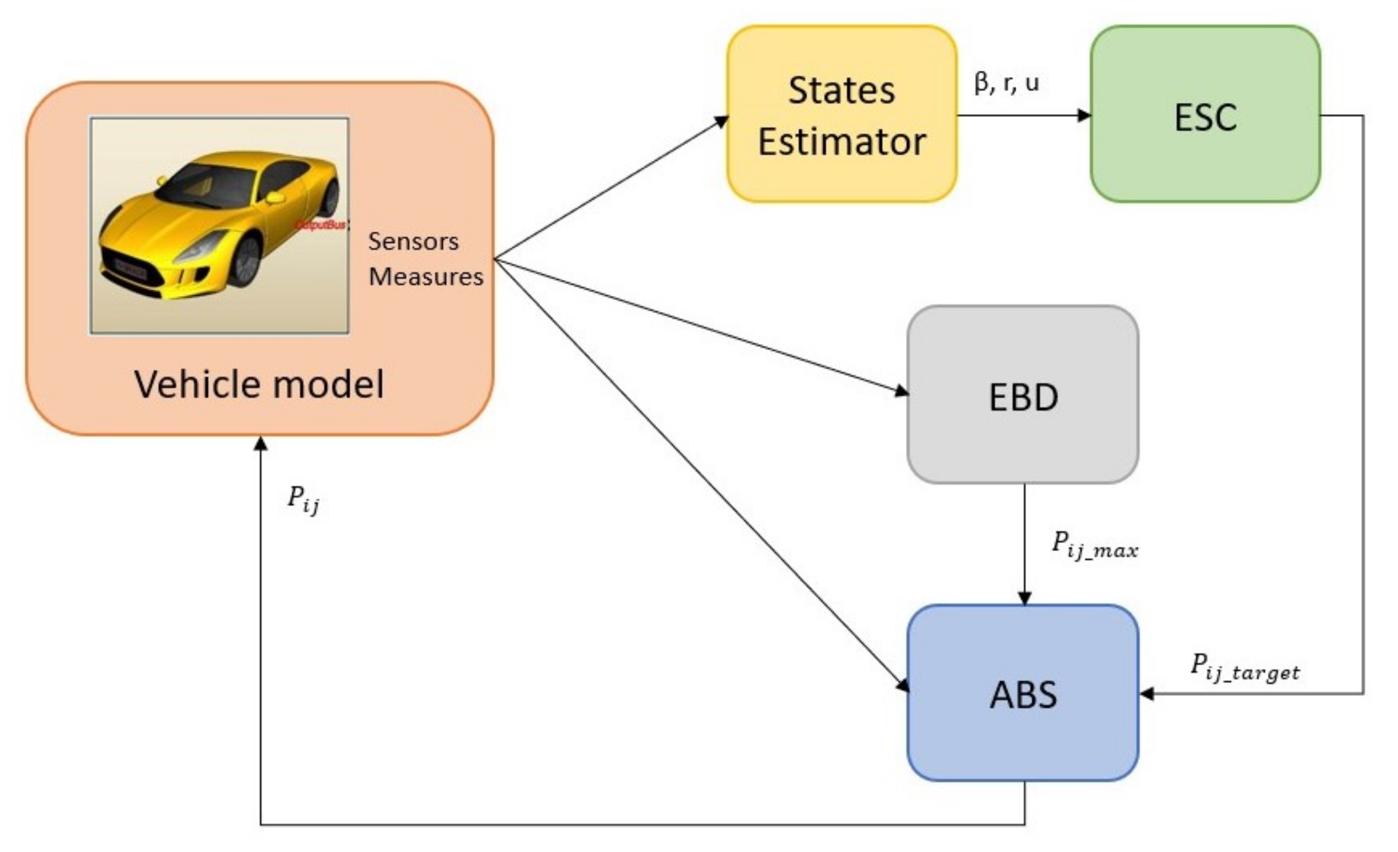
The three types of ABS share the same aim and interact with the entire architecture in the same way; the $ABS$ has as inputs the braking pressure required by the driver via the brake pedal, and the braking pressure required by the stability control system, $ESC$, through the wheels longitudinal forces that allow the car to achieve the yaw moment that stabilizes dynamics. Instead, the $ABS$ outputs are the four wheel pressures that $CBA$ units must provide to the callipers to improve performance by ensuring input requirements. Therefore, the $ABS$ input target pressure is defined by: the percentage-to-pressure coefficient that converts driver pedal input, $Pedal$, to requested pressure, $P_t$ ($Pa$), matching the 100% with the maximum pressure that the actuators can reach, $P_{max}$, as shown in Equation (1); and the force-to-pressure coefficient, $c_p$, that as a function of the braking piston’s area and braking piston’s friction, converts longitudinal forces requested by the $ESC$, $F_d$, into pressure, $P_d$ ($Pa$), as shown in Equation (2).

$$P_t=P_{max}*Pedal$$

(1)

$$\begin{array}{ccc}{P}_d=\frac{F_d}{c_p};& & c_p=A_p*\mu \end{array}$$

(2)

All three $ABS$ logics work with a sample time of 0.001 s, and disable their control when the car speed is under 2 m/s. This switch-off is necessary to improve braking performance without threatening stability. In effect, when vehicle speed is low, the brake actuator can provide its maximum potential without risks.

Since the study involves sensitive data all the tuning parameters and gains used can’t be shown and only the formulations and functions implemented will be presented.

3.1. Standard ABS

By using the name, ‘standard’, it is highlighted that the longitudinal control includes logic that is already available in all commercial vehicles. This logic works as a bang-bang control, where the braking pressure of the callipers is increased, decreased, or held depending on the wheel acceleration value.

So, a Standard ABS was developed trying to obtain the same results as the system developed by Bosch [16]. It is composed of an algorithm that raises, maintains, or reduces pressure (w.r.t. driver pressure demand) as a function of two states: wheel acceleration, $\dot{\omega }$, and measured vehicle longitudinal speed, u. The measured vehicle speed is the vehicle longitudinal speed estimated by integrating the car’s longitudinal acceleration. To avoid the drift in estimation due to a little bias of the acceleration, the integration is reset to the mean value of the four wheel speeds thanks of the pulse function $g\left(t\right)$ of 0.1 s width and 1 amplitude value, as shown in Equation (3).

$$u_i=a_i*dt+c\left(g\left(t\right)\right)=\left\{\begin{array}{cccc}c\left(g\left(t\right)\right)=u_{i-1}& if& g\left(t\right)=0& \forall i=1,2,\dots T\\ c\left(g\left(t\right)\right)=mean\left({\omega }_{ij}\right)& if& g\left(t\right)=1& \forall i=1,2,\dots T;\forall j=1,2,3,4\end{array}\right.$$

(3)

So, two threshold bands are defined, which depend not only on the wheels’ acceleration, as usual, but also on the wheels’ speed. These thresholds smooth out the controller action, improving the $ABS$ performance respect the one that controls only the wheels acceleration.

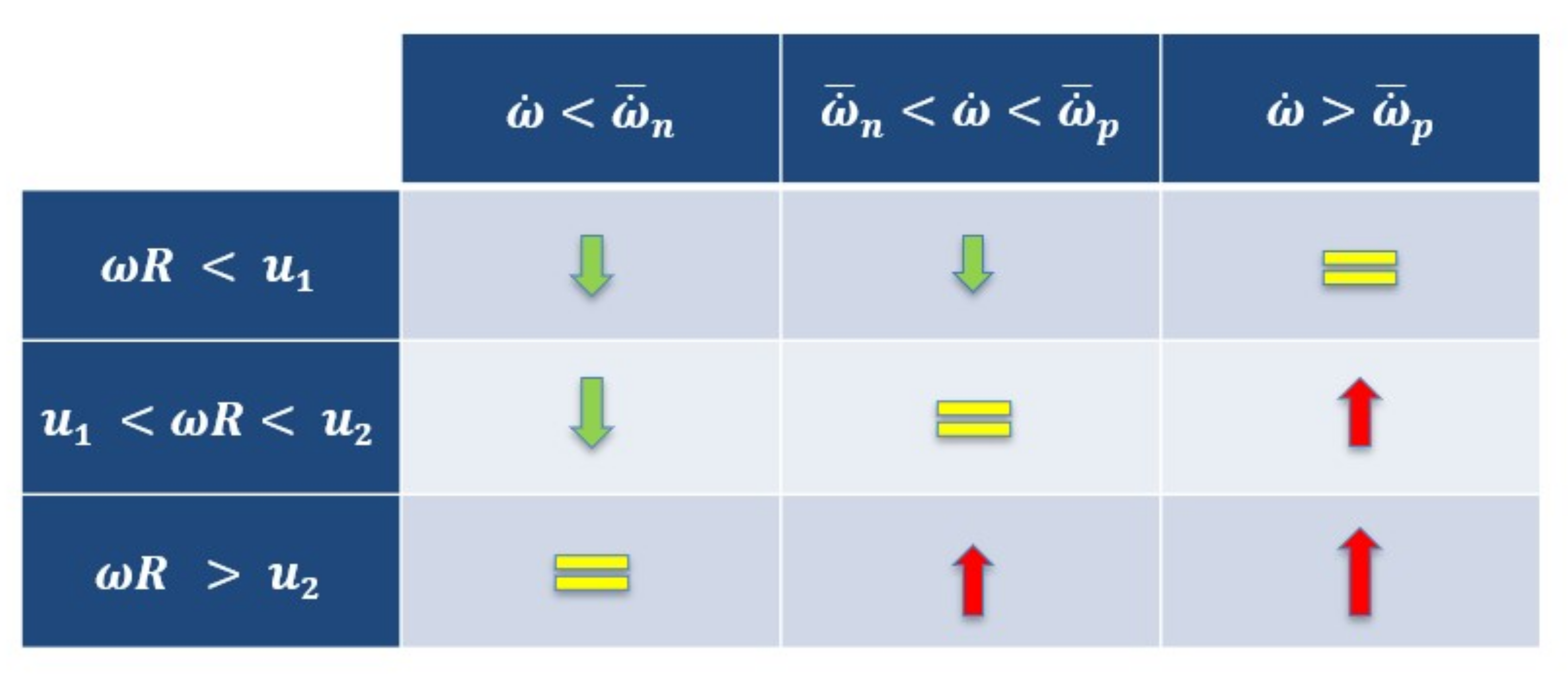
Figure 2 shows the logic used. Nine sectors divide the $ABS$ work, and each sector depicts: a reducing of pressure with the green arrows; a raising of pressure with the red arrows; and a holding of pressure with the equals sign.

The band threshold defined by $u_1$ and $u_2$ ensures that the different between the vehicle speed and the wheel speed, i.e., the slip velocity, does not exceed the percentage distance, $u_2=k_2*u$, from the saturated value of the tire by reducing pressure. At the same time, the acceleration performances are improved by holding and increasing the pressure if the slip velocity is inside $u_2=k_2*u$ and $u_1=k_1*u$ or above $u_1=k_1*u$. Instead, the threshold band defined by $\overline{{\dot{\omega }}_p}$ and $\overline{{\dot{\omega }}_n}$ avoids the risk that longitudinal wheel speed declines quickly to zero controlling that the slip does not reach the saturation limit.

The tuning process has involved the definition of the threshold parameters, $k_1$, $k_2$, $a_{xm}$ and $a_{xp}$ by physical observation and formulation, shown in

Table 1. ABS threshold definition.

Variable	Value
$u_1$	$k_1*u$
$u_2$	$k_2*u$
$\overline{\dot{{\omega }_n}}$	$\frac{1-{\sigma }_t}{R}*a_{xm}$
$\overline{\dot{{\omega }_p}}$	$\frac{1-{\sigma }_t}{R}*a_{xp}$

, and nine pressure slops by trial and error approach. The speed thresholds were defined trying to maximize the brake pressure capabilities and avoid to lock the wheel. So, it was supposed that if the 90% of the slip velocity ensures a near to maximum longitudinal wheel force, a difference of the wheel speed from the vehicle speed bigger than a 80% could cause a saturation of the tire. Regarding wheel acceleration thresholds, they were established by the physical formulation shown in Equation (4) where the slip ratio function is derived by considering a fixed target slip, ${\sigma }_t$ and the wheel radius, R. The minimum deceleration value of the wheel was estimated using $a_x=a_{x}m$, that is the maximum absolute longitudinal deceleration that the vehicle can express. Instead, the positive upper acceleration threshold was estimated using $a_x=a_{x}p$, that is a tuning parameter.

$$\begin{array}{ccccc}{\sigma }_t=\frac{u-\omega *R}{u};& & \omega =\frac{1-{\sigma }_t}{R}*u;& & \dot{\omega }=\frac{1-{\sigma }_t}{R}*a_x\end{array}$$

(4)

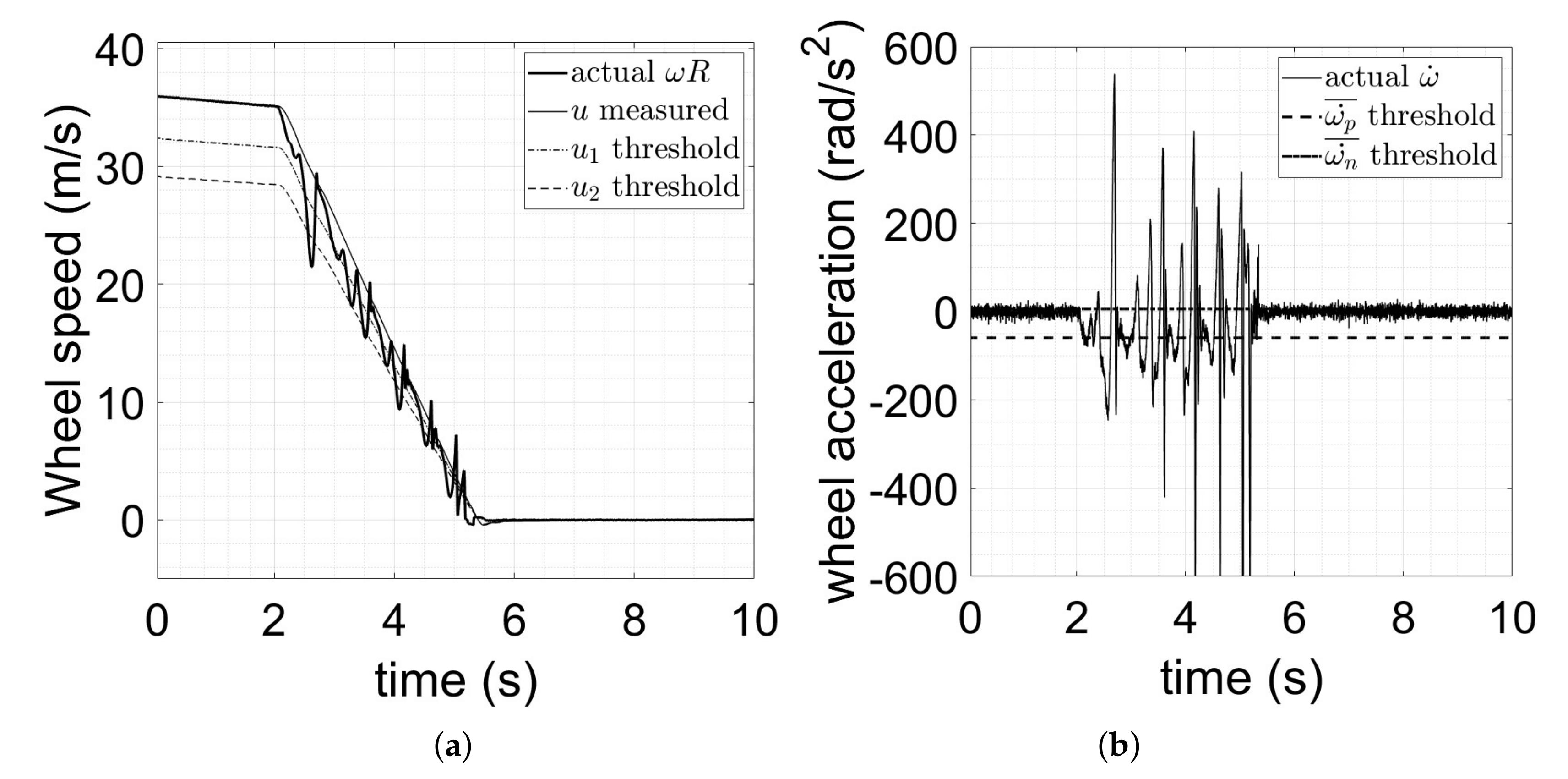
The brake pressure slopes were defined by a trial and error process at the simulator with the aim to obtain a robust and repeatable behaviour in term of avoiding wheel locking and maximizing the performances by smoothing out the signals. In fact, a maximization of the performance in high friction condition did not ensure a safety and effective braking in low friction condition, where the signal oscillations prevented to increase the pressure slop. However, depending on the designer’s requests, it is possible to adjust the upward and downward pressure rates to obtain higher performance under certain conditions, not ensuring a continuity of performance in all the dynamic or contact condition. The tuning process work is shown in Figure 3.

It is important to point out that the slopes of decreasing and increasing pressure change depending on the speed of the vehicle: when it is travelling faster than 50 km/h, the slopes have one value; when it is slower than 50 km/h, they have a different value. This schedule was necessary because during the tuning phase on several manoeuvres, the use of unique gradients did not guarantee the correct operation of the vehicle at low speeds.

3.2. Slip Controller

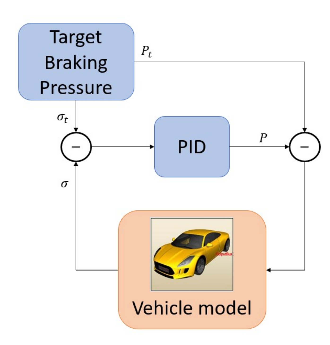
However, the Standard ABS is a bang-bang control, so it has a noisy behaviour that is not comfortable for passengers and results in lower efficiency, also involving a long tuning process. So, an $ABS$ was developed that could track the longitudinal slip of the tire, as Johansen et al. [13], ensuring a continuous control of the braking pressure. The Slip Controller aims to minimize the error between the wheels’ actual and target longitudinal slip, and its working structure is shown on Figure 4. In this Figure, the Target Braking Pressure block provides: the target pressure, $P_t$, requested by the driver and calculated by Equation (1); and the target longitudinal slip, ${\sigma }_t$ calculated as function of the target braking pressure as follows:

$$F_{xt}=-c_p*P_t$$

(5)

$${\sigma }_t=f\left(F_{xt}\right)$$

(6)

where $c_p$ is the force-to-pressure coefficient defined in Equation (2), and $f\left(F_{xt}\right)$ is the longitudinal tire characteristic found with the tire testing event of Car-Real-Time ($CRT$) at a normal load of 3000 N. To ensure that the controller works only when the wheel is braking, and not when it is in traction, the ${\sigma }_t$ is saturated between 0 and −0.1. This range ensures that the wheel slip is such as to have the greatest longitudinal force, and therefore braking pressure, without reaching the wheel lock, i.e., maintaining a certain margin from the 100% of slip.

About the actual value of the car longitudinal slip, $\sigma$, it is estimated by the following formulation:

$$\sigma =-\frac{v_{xij}-{\omega }_{ij}*R_{ij}}{v_{xij}}$$

(7)

where i stands for front or rear and j left or right values; the $v_{xij}$ is the longitudinal wheel speed as function of the longitudinal, lateral and rotational vehicle speed; and ${\omega }_{ij}$ and $R_{ij}$ are respectively the angular wheels speed and the wheels radius.

So, as shown in Figure 4 the error between the target, ${\sigma }_t$, and actual, $\sigma$, longitudinal slip represents the input of the discrete $PID$ which thanks of the tuning three gains, $K_{i,p,d}$, and working at a sample time of 0.001 s, minimize the proportional, derivative and integral errors of the residual of the states, defining the pressure P to be subtracted from the target one $P_t$.

The main problem of this control is the slip estimation. In fact, if for the Standard ABS is sufficient a measure of the speed, to have a satisfactory longitudinal slip estimation and so a good performance of the Slip Controller, a precise longitudinal vehicle speed relative to the wheel it is necessary. As shown in Figure 5, because of the small values that the slip has, a small error on speed estimation, in the order of cm/s, leads to a large error on slip estimation. This error has the same order of magnitude of the quantities in question. If in high friction condition the errors are not relevant, in low friction condition they influence the Slip Controller functionality reducing the performance of the braking. For the same reason, i.e., because it is a small size compared to the longitudinal speed, the noise in the wheel sensors has a significant influence on the slip estimation and therefore also on the operation of the Slip Controller.

As for the Standard ABS, to ensure the correct operation of the controller at low speed, the discrete $PID$ was scheduled with the longitudinal speed of the vehicle (e.g., when u is less than 36 km/h, the gain values are significantly reduced).

3.3. Wheel Speed Controller

If the Slip Controller ensure a smoother behaviour than Standard ABS, maintaining a certain level of performance in nominal contact path, involves estimating the longitudinal slip and therefore the longitudinal and lateral speed of the vehicle as accurately as possible to ensure the same performance at degraded contact path. But, with the current sensors and technologies a certain error is achieved in combined slip if the tire is near to the saturation, and when the contact condition are not the nominal one (reduced friction condition). For these reasons, a novel type of $ABS$ was developed linking together the two longitudinal controls showed. So, to guarantee a tracking of the braking pressure, a discrete $PID$ controller with a sample time of 0.001 s was chosen; and to not need of estimated values, the wheel speed was chosen as the state to be controlled by measuring its value with sensors and not with an estimation model.

The architecture of the controller is the same of the Slip Controller shown in Figure 4, but instead of a target longitudinal slip, the discrete $PID$ controller has to minimize the error between the wheel speed and a reference value, $u_2$, defined as a percentage of the measured vehicle speed, u, as for the Standard ABS:

$$u_2=k_2*u$$

(8)

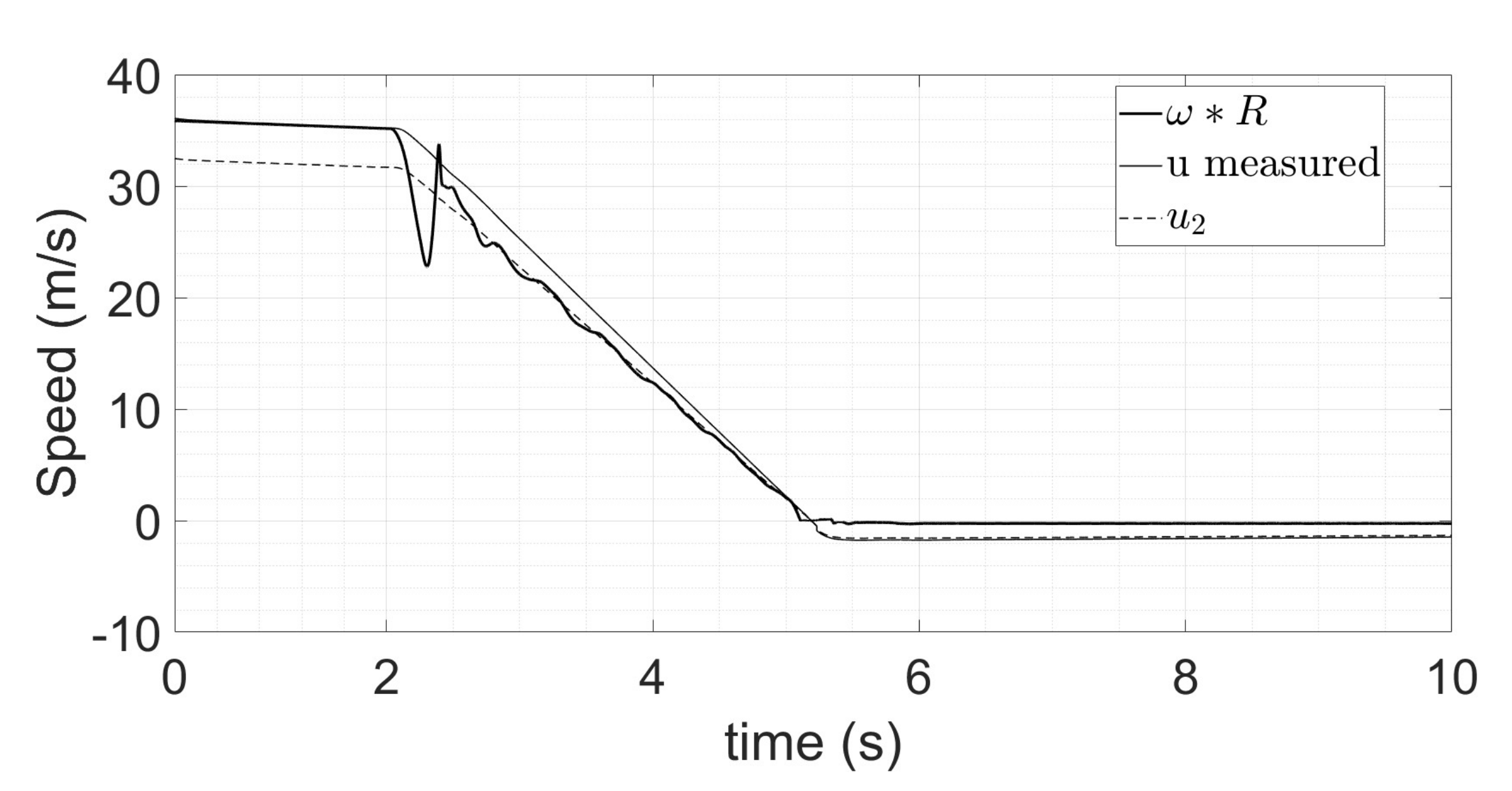
The u is calculated by Equation (3) and $k_2$ is a tuning parameter that defines the target speed value that the wheel must have to avoid locking and ensure the deceleration required by the driver, as shown on Figure 6. In this Figure, the measured speed, u, does not stop at zero m/s due to the car body movements at its stop detected as positive acceleration. However, the algorithm works with a saturated u that must be greater than or equal to zero.

The continuous-time $PID$ formulation is the one shown in Equation (9) with its Laplace transform shown in Equation (10). However, to consider the signals transmitted inside the car the Discrete $PID$ formulation, obtained with the backward Euler methods for both the integral and derivative terms and shown in Equation (11), was used and implemented.

$$u_{\left(t\right)}=K_p{e}_{\left(t\right)}+K_i{\int }_0^t{e}_{\left(\tau \right)}d\tau +K_d\frac{d}{dt}{e}_{\left(t\right)}$$

(9)

$$C_{\left(s\right)}=K_p+\frac{K_i}{s}+\frac{N{K}_d}{1+N/s}$$

(10)

$$C_{\left(z\right)}=K_p+\frac{K_{i}Tz}{z-1}+\frac{N{K}_d(z-1)}{(1+NT)z-1}$$

(11)

So, $\left(z\right)$ is the discrete time variable in the Z-Domain and the input of the discrete $PID$, $I\left(z\right)$, is the error e described in Equation (12). Its value will be reduced by tuned $PID$ parameters, $K_p$, $K_i$ and $K_d$ that through the formulations shown in Equation (13) define the discrete $PID$ output, $U\left(z\right)$: the braking pressure, $P_t$ to be subtracted to the pressure requested by the driver ensuring that the wheel does not lock.

$$e=(u_2-\omega *R)$$

(12)

$$\begin{array}{cc}\hfill C_{\left(z\right)}& =\frac{U\left(z\right)}{I\left(z\right)}=\frac{B_0+B_1{z}^{-1}+B_2{z}^{-2}}{A_0+A_1{z}^{-1}+A_2{z}^{-2}}\hfill \\ \hfill B_0& =K_p*(1+N*T)+K_i*T*(1+N*T)+K_d*N\hfill \\ \hfill B_1& =-(K_p*(2+N*T)+Ki*T+2*K_d*N)\hfill \\ \hfill B_2& =K_p+K_d*N\hfill \\ \hfill A_0& =1+N*T\hfill \\ \hfill A_1& =-(2+N*T)\hfill \\ \hfill A_2& =1\hfill \\ \hfill P_t& =-\frac{A_1}{A_0}*P_1-\frac{A_2}{A_0}*P_2+\frac{B_0}{A_0}*e+\frac{B_1}{A_0}*e_1+\frac{B_2}{A_0}*e_2\hfill \end{array}$$

(13)

In Equations (13), the discrete dynamic control system is shown and in addition to the parameters already defined are present: T that represents the sample time of 0.001 s; N is the low-pass filter parameter, to make derivative term less noisy, and usually has the value of 100; $B_0$, $B_1$ and $B_2$ are the numerator coefficients of the discrete transfer function, $\frac{U\left(z\right)}{I\left(z\right)}$; $A_0$, $A_1$ and $A_2$ are the denominator coefficients of the same transfer function; $P_1$ and $P_2$ are the output values at the time $(t-1)$ and $(t-2)$ considering that t is the current time step; and $e_1$ and $e_2$ are the input values at the time $(t-1)$ and $(t-2)$. Compared to the other longitudinal controllers presented this one has not been needed of a scheduling with the longitudinal vehicle speed. Thus, its tuning process was quicker and more simple due to the definition of only three parameters, $K_p$, $K_i$ and $K_d$.

4. Tests and Results

Figure 7 shows the Hardware-In-the-Loop ($HiL$) simulator used to test the three control logics developed. The simulator is a real-time car simulator of VI-grade and is located at Meccanica 42.

This simulator uses a complex car model of 14 Degrees Of Freedom ($DOF$) developed in $CRT$ software, and it can complete a co-simulation with the Matlab-Simulink environment, where the logic’s sub-models are implemented, as seen in Section 2. The $CBA$’s performance was evaluated on a test bench by performing a set of actuator response tests at a pressure step between 0 and 100 bar. From these tests, it was implemented an appropriate transfer function to represent the brake actuators’ operation. Furthermore, during experimental tests on the car without the control architecture, a sensors characterization was made and thanks of it, it was possible to add at the input values a white noise and simulate the transmission of signals that will take place inside the car.

Two types of manoeuvres under different asphalt surface conditions were carried out to evaluate the $ABS$ response. They are:

• Longitudinal braking;
• Combined braking.

Table 2. Manoeuvres’ characteristics.

	Longitudinal Braking		Combined Braking
Friction level	1.0	0.7	1.0	0.7
Longitudinal speed	130–80 (km/h)	130–80 (km/h)	80 (km/h)	80 (km/h)
Lateral acceleration	0 (g)	0 (g)	0.9–0.5 (g)	0.5 (g)

summarizes their specific characteristics.

From the tests, the results highlighted the capability of all three $ABS$ to avoid wheel locking, reduce braking distance, maintain a stable trajectory, and improve deceleration level.

The results below show sensitive data. For this reason, they are normalized with respect to the values of the model without controls and are shown, for the sake of brevity, only the graphs of longitudinal braking manoeuvres at 130 km/h with friction levels of 1.0 and 0.7, and combined braking manoeuvres at 0.9 g with a friction level of 1.0. However, in Section 4.3 the results of all the manoeuvres are described and commented on.

4.1. Longitudinal Braking

The ISO standard [17] states that the longitudinal braking manoeuvre used to test the $ABS$ control must establish if it is able to prevent the wheels from locking and give more stability to the car. The manoeuvre consists of starting from a certain longitudinal speed and braking sharply until the vehicle comes to a complete standstill. The driver’s braking has a pressure increase slope of 1000 bar/s. The authors tested the same manoeuvres with a friction level of 0.7 to assess its performance in slippery conditions.

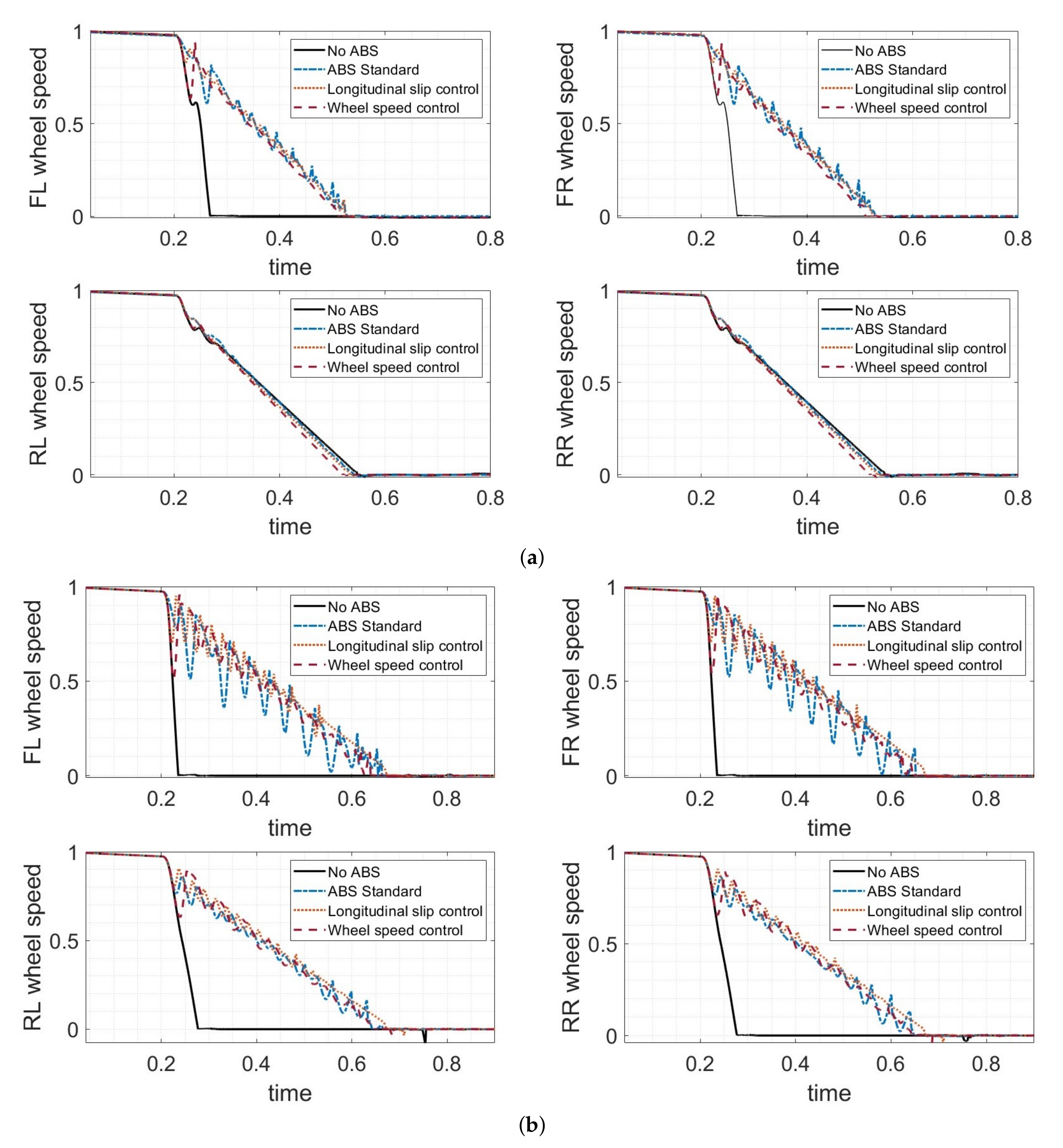
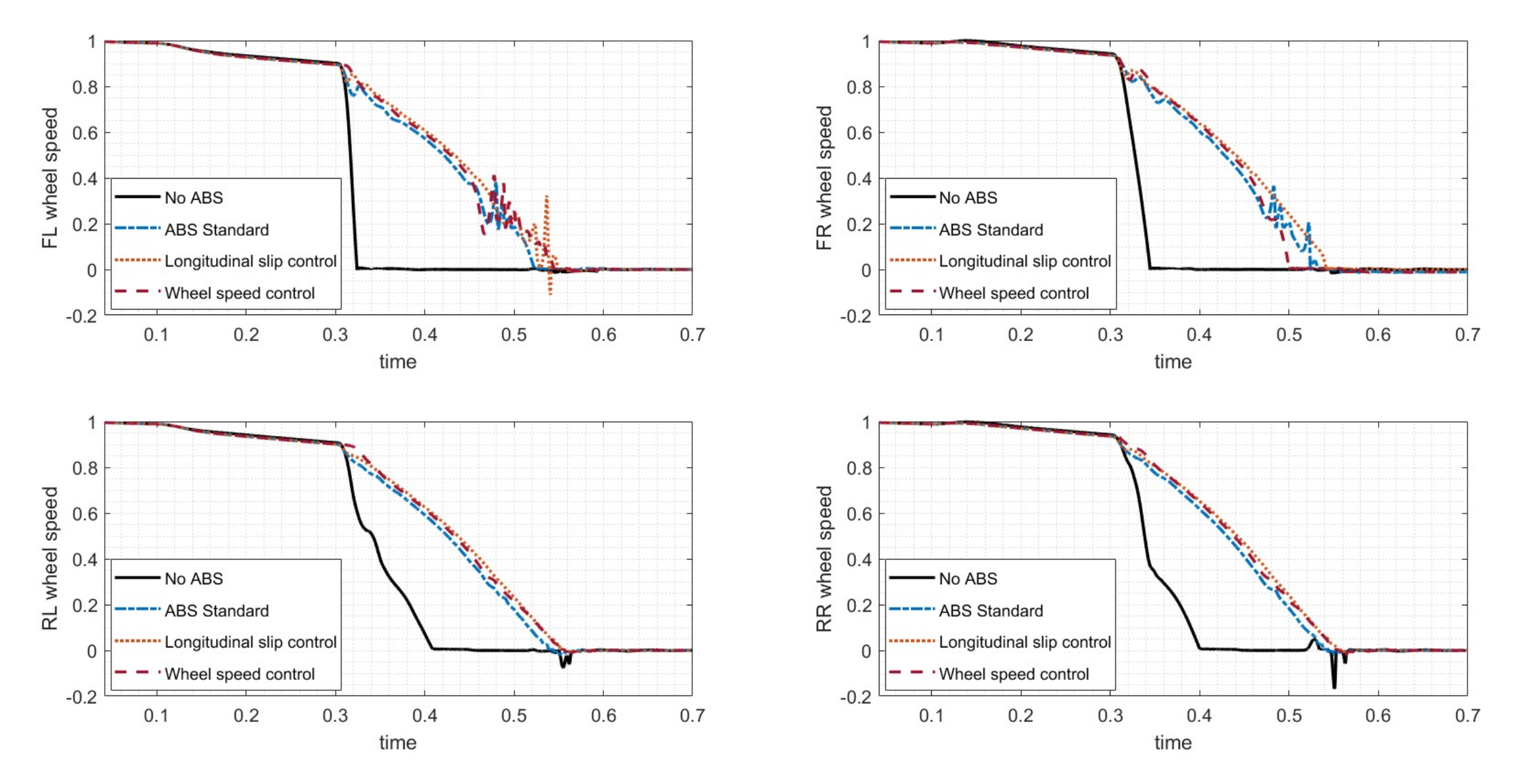
Figure 8 shows the wheels’ speeds from the starting speed to when the vehicle is completely stationary in nominal (a) and reduced (b) friction condition. It shows that the absence of the $ABS$ leads to the locking of the front wheels, or all wheels when friction is 0.7. On the other hand, the presence of any of the three types of $ABS$ makes it possible to avoid locking. However, the Standard ABS compared with the Slip Controller and the Wheel Speed Controller has a chattering behaviour, especially in reduce friction condition, reducing the performance and adding noise to the all system.

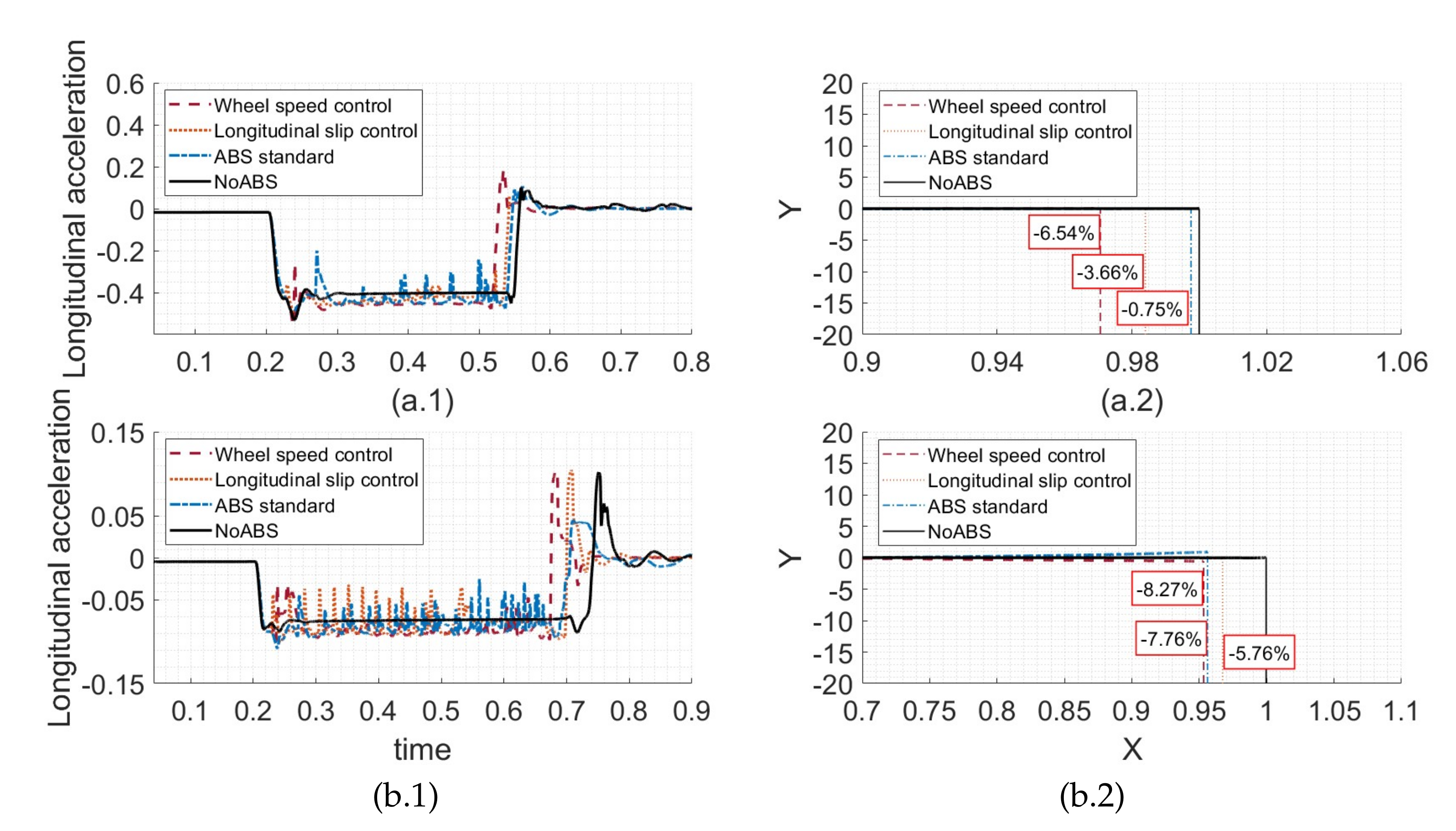
These results are confirmed in Figure 9, that shows in (a.2) and (b.2) the car’s trajectory until the vehicle is stationary and in (a.1) and (b.1) the longitudinal deceleration of the car in nominal, (a), and reduced, (b), friction condition. The values shown are normalized with respect to the maximum longitudinal distance, and longitudinal deceleration achieved by the car without controls. The numbers inside the red rectangles represent the percentage of reduction in braking distance compared to the vehicle without controls and underlined that the Wheel Speed Controller is able to achieve a shorter braking distance of the others reaching almost double the reduction of the other controls under nominal friction conditions. It is also interesting to note that if in nominal friction condition the Slip Controller has better performance than the Standard ABS, thanks of its smoother behaviour, in reduced friction condition its performance go worse in terms of braking distance because of the multiple estimated values involved (longitudinal speed, longitudinal force and longitudinal slip). So, the Wheel Speed Controller has less braking distance than other controllers, even if it shows a small right side-shift in the case of the slippery surface. However, this shift still allows the car to stay inside the roadway without risk of danger. Furthermore, about the car’s longitudinal acceleration the three longitudinal controllers tested allow the car to reach higher decelerations than the case without $ABS$ and in both contact conditions, the smoother behaviour of the Wheel Speed Controller ensures to maintain higher longitudinal deceleration and for this reason the braking distance is reduced. This behaviour is useful especially when the friction is 0.7, whereas Standard ABS and Slip Controller act in a very noisy way because of quick on-off switches, and a poor estimate of the tire contact conditions respectively.

4.2. Combined Braking

This manoeuvre underlines the ability of the $ABS$ to ensure that the vehicle follows the driver’s inputs as neutrally as possible, avoiding a loss of control from over-steering or under-steering and the wheels locking. It starts with a steering ramp up to the desired lateral acceleration and then a sharp braking from the start speed to when the vehicle is completely standstill.

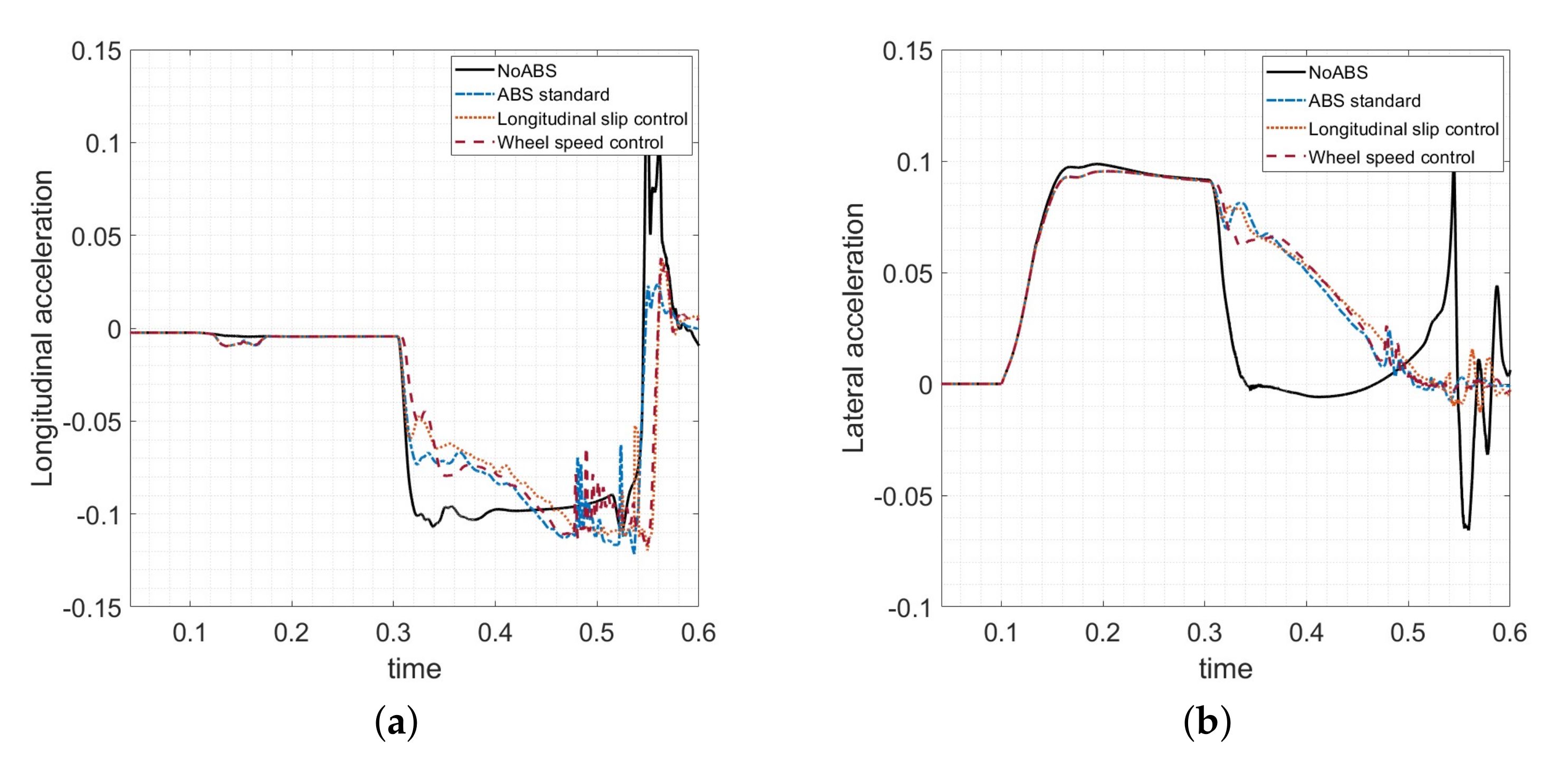
Figure 10 shows that the wheels do not lock only with the action of three $ABS$ controls. Moreover, all three longitudinal controls can provide linear lateral deceleration in front of an increase in longitudinal acceleration, instead, the absence of $ABS$ leads to a sudden loss of lateral acceleration with the following loss of stability as is shown in Figure 11.

In Figure 12, the trajectory of the car during the manoeuvre, (a), and its zoom from when braking starts until the end of the manoeuvre, (b), are shown comparing the radial distance achieved by the three controllers from reference trajectory. The reference trajectory represents the constant radius path, which allows the car to maintain the target lateral acceleration at the target speed, and for this manoeuvre is $\frac{{\left[22.2(\mathrm{m}/\mathrm{s})\right]}^2}{9({\mathrm{m}/\mathrm{s}}^2)}$. The graph shows this trajectory as a series of consecutive points. So, it shows that the Standard ABS achieves better performance than the others because it ensures the shortest radial distance, even if the performance of the three $ABS$ are very close and satisfactory allowing the vehicle to maintain the trajectory sets. In fact, the vehicle without control loses its stability by spinning out.

4.3. Complete Results

In

Table 3. Test results about braking distance performance.

		Longitudinal Braking				Combined Braking
		Friction				Friction
		1		0.7		1		0.7
		Speed (km/h)				Lateral Acceleration (g)
		130	80	130	80	0.9	0.5	0.5
Standard ABS	Braking distance	−0.75%	2.25%	−7.76%	−2.03%	0%	0%	0%
Slip control	Braking distance	−3.66%	−0.41%	−5.76%	1.78%	0.3%	−0.9%	0.01%
Wheel control	Braking distance	−6.54%	−3.90%	−8.27%	−3.9%	−0.4%	−1.5%	−0.7%

and

Table 4. Test results about radial distance performance.

		Longitudinal Braking				Combined Braking
		Friction				Friction
		1		0.7		1		0.7
		Speed (km/h)				Lateral Acceleration (g)
		130	80	130	80	0.9	0.5	0.5
Standard ABS	Radial distance	90%	9.2%	9%	50%	−99.3%	−70.2%	−69.2%
Slip control	Radial distance	58%	8.6%	0.7%	80%	−96.3%	−69.8%	−73%
Wheel control	Radial distance	99%	3.2%	5.5%	85%	−91.7%	−60.3%	−62%

can be determined which type of $ABS$ ensures the best performance in a wider range of manoeuvres.

In the columns, the characteristics of the manoeuvres are defined as: the type, longitudinal or combined; the friction level, 1 or 0.7; the car’s speed, 130 km/h or 80 km/h; and the car’s lateral acceleration, 0.9 g or 0.5 g. As a friction level of 0.7 limits vehicle dynamics, only combined braking manoeuvres with a car’s lateral acceleration less than 0.5 g was done.

Instead, in the rows, are indicate the type of $ABS$ algorithm that equips the car (Standard ABS, Slip controller, and Wheel Speed controller) and the performance considered (braking distance and radial distance).

The negative values shown in the table are the percentage reductions of the braking distance and radial distance respect the vehicle without longitudinal control, instead the positive ones are the percentage increases. The red values specify when the car had the lowest braking distance in longitudinal braking, and the lowest radial distance from the constant radius reference trajectory in combined braking. Thus, as it possible to see in Table 3, the results obtained by the controllers in the longitudinal braking manoeuvres show that in high friction conditions the Standard ABS has a little percentage improvement at 130 (km/h) and even an increase in braking distance at a speed of 80 (km/h) due to an increase in the oscillating behaviour of the controller, instead in low friction conditions the brake distance is ensured in both 130 and 80 (km/h); regarding Slip Control $ABS$, it allows a greater reduction in braking distance compared to the Standard ABS in high friction conditions. Instead, in low friction conditions its performance gets worse because of the estimation errors seen in Section 3.2. At the speed of 80 (km/h), these estimation errors increase the braking distance compared to the vehicle without controller; the performances of the Wheel Speed Control are the most effective in terms of reducing the braking distance, ensuring continuity of behaviour when subjected to different speeds and different road contact conditions.

In Table 4, the radial distance of the longitudinal braking manoeuvres represents the lateral deviation of the vehicle at the time of stopping. The three controls show a high percentage value of increase in lateral distance compared to the vehicle not equipped with ABS. This is because, since all the actuators have the same pressure target, the car without longitudinal control reaches lateral displacements of the order of a millimetre in high friction or centimetre in low friction, so even if in the other controls the car moves sideways by a few centimetres or tens of centimetres the percentage increase is very large. However, all three controls in the different types of manoeuvres have a lateral displacement due to a different pressure distribution on the right and left wheels of less than 20 cm.

Whereas, the results obtained by the longitudinal controllers and presented in Table 4 for the combined braking manoeuvres show a decisive percentage reduction in the radial distance from the reference trajectory. It happened because during braking the car without controls saturates the wheels and turns. In this case, the ABS developed ensure that the vehicle maintains the set trajectory by increasing the stability of the vehicle both on dry and wet surface.

The braking distance performance in combined braking manoeuvres, shown in Table 3, is calculated as reduction or improvement percentage respect the Standard ABS, because the car without control spins out and so its trajectory is not a good comparison metric. In this case, the difference between the three controllers is in the order of a few centimetres.

5. Conclusions

In this paper, the authors have shown the different behaviour of three types of a car’s longitudinal control, $ABS$, which they developed in order to choose which should be implemented on a dSpace inside a car prototype with the characterized sensors shown in Section 2. The tests done have been involved the use of a co-simulation environment between $CRT$ and Matlab-Simulink, where the three types of controllers have been incorporated inside an architecture control logic composed of a state estimator, an $ESC$, an $EBD$, and a $CBA$ model. The aim of the activities carried out was to ensure safety, improve the performance of the braking system during full braking manoeuvres by ensuring the driver a vehicle response as close as possible to his requirements with an integration that allows all the systems involved to work at their best and with a sampling time of 0.001 s.

The figures shown and Table 3 and Table 4 allow to say that all the types of longitudinal controller developed avoid wheel locking and ensure less braking distance compared to the car operating without $ABS$. In addition, the combined braking tests show that the vehicle remains stable and steerable in wheel saturation limit conditions thanks to the longitudinal control actions.

However, the Wheel Speed controller is preferred for the following reasons: it exhibits a continuity of performance in all conditions under which it has been tested; compared to the Standard ABS it allows $CBA$ to track the braking pressure in continuous and have a smoother behaviour both in dry and wet surface, ensuring a less disturbing intervention and, therefore, more comfort for passengers; compared to the Slip Control it does not have necessary of estimated tire longitudinal slip that are functions of the tire conditions and run into errors in low friction conditions that compromise the $ABS$ operation; and having only three parameters, $K_p$$K_i$$K_d$, that define its functionality it allows a simpler and faster tuning process compared to both the other controllers providing easy integration and implementation of the system in current cars.