Abstract
As a result of the increased integration of power converter-connected variable speed wind generators (VSWG), which do not provide rotational inertia, concerns about the frequency stability of interconnected power systems permanently arise. If the inertia of a power system is insufficient, wind power plants’ participation in the inertial response should be required. A trendy solution for the frequency stability improvement in low inertia systems is based on utilizing so-called “synthetic” or “virtual” inertia from modern VSWG. This paper presents a control scheme for the virtual inertia response of wind power plants based on the center of inertia (COI) frequency of a control area. The PSS/E user written wind inertial controller based on COI frequency is developed using FORTRAN. The efficiency of the controller is tested and applied to the real interconnected power system of Southeast Europe. The performed simulations show certain conceptual advantages of the proposed controller in comparison to traditional schemes that use the local frequency to trigger the wind inertial response. The frequency response metrics, COI frequency calculation and graphical plots are obtained using Python.
1. Introduction
Over the last ten years, the structure and control of the electric power system (EPS) have changed dramatically due to the increased integration of variable power generation (from wind and photovoltaic solar) [1]. In 2019, 15.4 GW of new wind power plants (WPP) had been installed and connected to the European power system, so the total installed capacity of WPP in Europe reached 205 GW [2]. Southeast Europe (SEE) region is also experiencing a “wind boom”. The total installed capacity of WPP in 2019 in the SEE reached 5 GW. The largest number of conventional power plants in the SEE region were built during the 1970s and 1980s. In the near future, due to carbon pricing (e.g., emissions trading system, carbon taxes or EU Carbon Border Adjustment mechanism) and the aging of conventional thermal power plants (TPP), it is expected that coal-fired TPPs will decrease production or will be decommissioned (e.g., the recent case of Romania). They will be mainly replaced by variable speed wind generators (VSWGs). Conventional generating units have an inherent property to support the grid frequency regulation since the generator’s rotating mass provides kinetic energy to the grid (or absorbs it) in the case of a frequency deviation caused by an active power imbalance.
Since VSWGs are connected to the network via power back-to-back AC/DC/AC converters, there is no direct electrical coupling between the grid frequency deviation and VSWG active power generation [3], which means that they do not contribute to the total system inertia. As the amount of wind energy in EPS increases, the share of connected synchronous machines and the total system inertia will decrease during high wind power generation periods. A detailed assessment of the dynamic impact of wind generation on EPS frequency control and changing system frequency behavior trends following the largest generator’s loss is studied in [4]. The assessment requires detailed modelling of an entire interconnection for different wind penetration and contingency scenarios [5]. Reduced total system inertia causes many challenges and research opportunities for frequency control of future EPS [6,7]. It has a direct impact on frequency stability, potentially leading to under-frequency load-shedding (UFLS) [8] or, in the worse cases, to system blackouts (e.g., the 2016 Australian blackout and the London blackout of 2019) [9,10]. From the EPS point of view, inertia is essential because inertia slows down the frequency change, giving balancing mechanisms more time to respond and stabilize frequency [11].
Modern power converter connected generation can provide inertia to the grid and support the frequency recovering process. The authors in [12,13] found that the virtual synchronous machine concept is a promising solution for improving the frequency response metrics in low-inertia EPS.
In the past few years, numerous strategies and control schemes have been developed to utilize WPP to inject additional active power during a frequency disturbance using synthetic or virtual inertia control [14,15,16]. A complete definition of synthetic inertia with a distinction from the general term of fast frequency response is well described in [17]. Synthetic inertia control is implemented to extract the kinetic energy stored in the wind turbine’s rotating blades and in wind generators, and is used to improve the quality of frequency response (FR) after a disturbance. The world wind industry has started to integrate controllers on modern VSWG to provide a temporary inertial response during frequency deviation (e.g., General Electric WindINERTIATM).
Emulated inertia controllers are mainly based on two different approaches: releasing hidden inertia and reserve capacity in pitch [18]. However, both methods have focused on developing inertial controllers that track frequency change at the point of common coupling (PCC) of WPP. Utilizing frequency at PCC as the input signal for the wind inertial controller will result in different synthetic inertial responses depending on the wind power plant (WPP) locations.
This paper presents the WPP inertial response control scheme based on tracking the selected control area’s center of inertia (COI) frequency. The control area is part of an interconnected system of the European Network of Transmission System Operators for Electricity (ENTSO-E). Usually, it coincides with a state’s territory, administered by a transmission system operator. The rationale behind the proposed scheme is based on frequency response (FR) analysis and the hierarchical organization of operation and control of continental European EPS [19]. The role of wind power and the need for additional inertia in the European EPS until 2050 was quantified in [20]. In [21], insufficient system inertia in European EPS has to be compensated by the provision of synthetic inertia.
The COI frequency is computed based on synchronous machine rotor speeds and widely used to define the effect of primary and secondary frequency regulation. Furthermore, COI frequency is particularly useful to present the frequency group of coherent synchronous machines. Regarding practical implementation, some previous researches considered that the COI signal is not fully adequate to support local frequency controllers due to delays in the communication system [22]. Nevertheless, modern digital high-speed telecommunication infrastructure brings new research opportunities and boosts the COI signal possibilities. Wind inertial control based on COI frequency can provide a “firm frequency response” within the first few seconds after the disturbance, regardless of their locations.
This paper aims to open the door for further research of frequency control based on COI in future low inertia system. The main paper contributions may be summarized as follows:
- The frequency response (FR) analysis of real interconnected EPS of the Southeast Europe region is performed and evaluated. The novel FR quality indicator “concentration of inertia” is introduced and calculated.
- The proposed wind inertial response control scheme based on the center of inertia frequency is introduced. The PSS/E user written wind inertial controller is developed using FORTRAN. The efficiency of the controller is tested and applied to the real EPS of SEE Europe.
The paper is organized as follows. In Section 2, the theoretical background of the power system frequency response is described. ENTSO-E inertia specifics are presented. A novel frequency response indicator is introduced. Next, in Section 3, the concept of COI is described. In Section 4, WPP contribution to the grid frequency regulation is explained. A proposed wind inertia controller based on the frequency of COI (FCOI) is presented in detail. In Section 5, a model of the SEE power system developed in PSS/E is described. The efficiency of the proposed controller is tested. Results of dynamic simulations, performed using PSS/E and supported by Python’s scripts, are presented. Finally, in Section 6, conclusions and some recommendations for future research are given.
2. Power System Frequency Response
The frequency of an interconnected electric power system is a fundamental quantity for estimation and control. The EPS must be operated within a safe frequency range. The frequency will remain at its standard value (e.g., 50 Hz in Europe) as long as active power from the generation and the load demand are balanced. The frequency quality parameters for the European Network of Transmission System Operators for Electricity (ENTSO-E) synchronous areas, continental Europe (CE), Great Britain (GB) and Nordic system (NO) are provided in Table 1 [23].

Table 1.
Frequency Quality Defining Parameters of the Synchronous Areas (Continental Europe (CE), Great Britain (GB) and Nordic system (NO).
According to the ENTSO-E, the interconnected power system of Continental Europe has to survive any frequency deviations due to a significant sudden change in load or generation (active power imbalance). The frequency response is the traditional metric used to describe how an EPS has stabilized frequency after the active power imbalance. To comply with the parameters given in Table 1, the FR process is realized through several phases: an inertial response, governor response (slow primary response) as illustrated in Figure 1, automatic generation control (secondary control) and tertiary control. In the initial phase of the incident (disturbance), which occurs during a few seconds (0–3 s) after the frequency changes, the synchronous generators’ rotor releases or absorbs part of its kinetic energy. The swing equation mathematically describes this process:
where, Hi (s) is the inertia constant of i-th turbine-generator, fi (Hz) is the frequency of i-th generator, f0 is the rated frequency, Pmi (p.u.) is the mechanical power of i-th turbine-generator, Pei (p.u.) is the electrical power of i-th generator and ΔPi (p.u.) is active power imbalance. Equation (1) shows an imbalance between the turbine generators’ mechanical and electrical power results in a frequency derivative. The rate of change of system frequency (ROCOF) is mostly used to evaluate the EPS frequency response dynamic. The ROCOF is directly proportional to the amount of active power imbalance:
where, Hsys (s) is the total system inertia constant, ΔP (p.u.) power imbalance of the system and f0 (Hz) system rated frequency. If the ROCOF becomes too high during a disturbance, it could lead to under frequency load shedding. The ROCOF is lower as the inertia of the power system is higher.
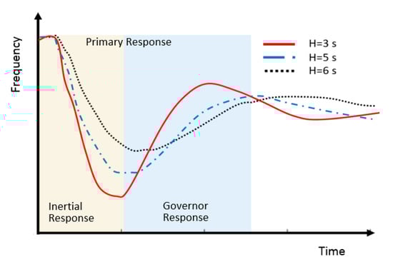
Figure 1.
EPS frequency response time frame with different total system inertia.
Large conventional generators (like coal, gas and oil-fired thermal power plants, nuclear and hydropower plants), which use synchronous machines to convert the mechanical power from their turbines to electrical power, are the primary sources of inertia in today’s EPS. Inertia constant H (s) describes the inertia of each generator:
where J (kg m2) is the moment of inertia of generator and turbine, ωn (rad/s) is the rotor angular speed and Sn (VA) is generator rated power. Inertia constant H falls typically in the wide range of 2–9 (s) [24]. The sum of all inertia of the spinning generators (and loads like motors) connected to the network is referred to as the total system inertia:
where Sni (MVA) is the rated power of the i-th generator, Sn,sys is system rated power equal to the sum of Sni and Hi (s) is the inertia constant of i-th turbine-generator. The number N in Equation (4) is the number of rotating synchronous generators connected to the system.
2.1. ENTSO-E Inertia Specifics
In Figure 2, the indicative inertia contribution of each European country (control area) at the time of the minimum total system inertia is presented. The contribution of SEE countries varies. Each country’s contribution depends on the generation portfolio and the number of connected conventional generators. Due to the low share of wind and PV solar in their generation portfolio, some countries (e.g., Serbia and BIH) have substantial inertia contributions. Others, like Greece and Croatia, have slightly lower system inertia. Generally, EPS’ stability and frequency control in the SEE region is still based on conventional power plants’ dynamic characteristics and controllability.
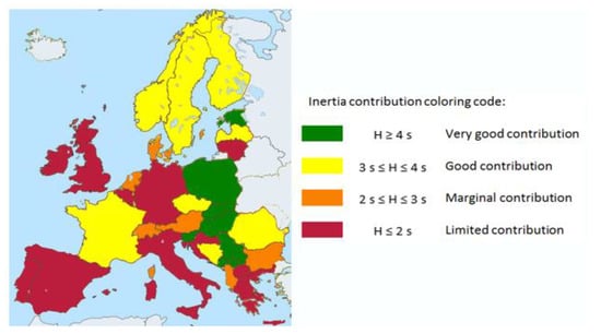
Figure 2.
Indicating the contribution of each Transmission System Operator (TSO) to the total system inertia (European Network of Transmission System Operators for Electricity (ENTSO-E)—Ten Year Network Development Plan 2016).
2.2. Novel FR Indicator—The Concentration of Inertia
Modern interconnected EPS with a high share of converter interfaced production units will need a sufficient amount of inertia (kinetic energy). Calculation and estimation of each real interconnected EPS’ available kinetic energy are crucial from the aspect of controllability and sharing inertial support among power systems. This paper introduced a novel FR metric called the “concentration” of inertia Hc (s). Instead of expressing inertia of a power system in seconds, it is often more convenient to calculate the kinetic energy stored in rotating masses of the system in megawatt seconds (MWs) [25]:
where Sni is the rated apparent power of generator i [MVA] and Hi is the inertia constant of turbine-generator 𝑖 (s).
This enhanced metrics (Hc) is determined using the ratio of the total kinetic energy and the total active power load (PL) in the individual EPS:
The proposed indicator—“concentration of inertia” characterizes each EPS and its contribution to the total system inertia. It is especially important that EPSs import electricity, and at the same time, have a significant share of wind in overall production. In the case of an imbalance that occurs in such EPS, a considerable part of the missing inertia will be provided from the interconnection. If the inertia (kinetic energy) of an EPS is low (small Hc), the participation of WPP in the inertial response should be required.
3. Center of Inertia Frequency Specifics
Real EPS consists of a large number of generators, and each of them, during the response to an active power disturbance, will operate at an individual frequency. Observing the entire system, there is an overall mean deceleration or acceleration of the fictitious center of inertia (COI) [26]. Individual generator frequency describes the power balance of the individual generator at a given location that is, due to electromechanical swings, oscillatory. In contrast, COI’s frequency describes an aggregated active power balance of the entire system, which does not contain electromechanical oscillations. The amplitude and slope of individual electromechanical oscillations of synchronous generators with respect to the COI frequency in the inertial phase of FR will depend on their turbine-generator models’ parameters and their electrical distance from the disturbance location. Based on the weighted average frequency (speed) of the individual generators, the frequency of the center of inertia can be calculated as:
The COI concept is the most common way to estimate the system frequency in transient stability analysis. The COI frequency could be calculated for a part of the interconnection, e.g., for a national EPS or a control area, which then contains inter-area electromechanical oscillations. Thus, the COI frequency is suited to study inter-area oscillations among coherent machine groups (clusters). In practice, instead of using COI, transmission system operators very often use the frequency estimated at a “pilot bus” of the system (typically a bus with a high short-circuit ratio). However, the “pilot bus” does not represent the system’s average frequency, as it follows the dynamics of the closest synchronous generators.
4. WPP Inertial Controller Based on COI Frequency of a Control Area
Since variable speed wind generators (VSWG) are connected to the grid via power converters, their rotational speed is isolated from the system frequency and does not contribute to the total system inertia. A controller that emulates a synchronous generator’s inertial response is often referred to as a synthetic, emulated, or virtual inertial response. Today, wind inertia controller activation primarily is based on the local frequency input signal. Using this type of controller, the active power output of VSWG is a function of the measured frequency and/or ROCOF. Estimating local frequency at PCC is commonly based on phase-locked loop (PLL) techniques. To emulate synthetic inertia, an initial additional active power ΔPi must be controlled with the following equation [27]:
where Pmax is the generator’s active power, Hgen is generator inertia constant and fn the nominal frequency. In order to emulate the inertial response properly, synthetic (virtual) inertia must be very fast (0–3 s). The exact values of the inertial constant vary depending on the manufacturer of WT. However, for research purposes, the WT inertial constant as a function of its power P (W) can be estimated [28]:
The total inertia of the wind turbine-generator system presents a sum of the inertia constant for the generator and the turbine. According to Equation (1), system frequency excursion in the inertial phase of disturbance is not the same in all system nodes. Utilizing the local frequency (at PCC) as the input signal for the wind inertial controller will result in different synthetic inertial responses depending on the wind power plant (WPP) locations.
Proposed Wind Inertial Control Scheme and Controller
The impact of emulated inertia on a real interconnected EPS frequency response is usually quantified and analyzed through time-domain simulations using commercial programs like Power Systems Simulation for Engineers (PSS/E) software. Unlike modelling classical thermal or hydro generating units, modelling of WPP is very specific. Wind turbine (WT) manufacturers develop their models, which are more or less complex, but substantially different. Modelling and transient stability simulations of EPS with many different WT commercial models could be hard work and quite frustrating. Generally, the idea is to create generic models that are parametrically adjustable to represent specific wind turbines available in the market. Developing a user-defined model and integrating it into a modular machine-model structure enables implementing a wide range of influencing factors in the power system dynamic simulations. PSS/E wind-related machine models with defined input-output dependencies can be integrated into the unique structure by developing a user-defined auxiliary signal model that controls the principle of operation of the entire model during the dynamic simulations.
The proposed wind inertia control scheme based on the control area’s COI frequency is presented in Figure 3. The input signal ΔωCOI presents deviation of the frequency of the COI of a control area with N synchronous generators, computed according to:
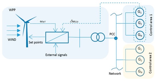
Figure 3.
Frequency of center of inertia (FCOI) wind inertia control scheme.
Based on the proposed scheme, a novel generic model of wind inertial controller FCPCAU1 is developed. The structure of FCPCAU1 is presented in Figure 4. FCPCAU1 is written in FORTRAN. PSS/E Environment Manager is used to compile code and create a dynamic linked library (DLL) [29]. The application of available wind generator and wind electrical PSS/E models combined with a user-defined wind auxiliary control model (FCPCAU1) implies the integration of the modified logic into the dynamic models’ structure. This inertial controller model is integrated with the existing generic wind electrical model REECAU1 and generic wind generator/convertor model REGCAU1. These models are contained in the PSS/E dynamics models library and they are widely used to represent Type 3, double fed induction generator (DFIG) or Type 4, fully fed generators.
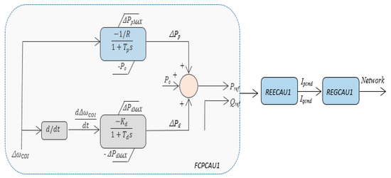
Figure 4.
FCPCAU1 wind inertia controller structure.
FCPCAU1 model storage, input and output parameters are presented with state variable values (STATE), real model parameters (CON) and real model variable values (VAR), as shown in Table 2 and Table 3.
Table 2.
FCPCAU1 Model Storage Parameters.
Table 3.
FCPCAU1 Model Input and Output Parameters.
FCPCAU1 controller consists of two modules: the first one performs droop control, while the second one performs inertia emulation. These two modules combined results in the recovery of the frequency to a new steady-state value. Adjusting model storage parameters (e.g., R), the droop controller module can be disabled. The droop module produces an active power change proportional to the frequency deviation. It is reasonable that R should be tuned on a similar value as conventional synchronous generators, Figure 5. The wind turbine generators (WTGs) usually operate at the maximum power point tracking (MPPT). The active power increase (ΔP) during a sudden drop of system frequency must be obtained from the kinetic energy of the rotating parts (turbine and generator) of WTG that causes a decrease of rotational speed. The droop control should be ended on time to avoid WT’s stalling or coordinated with the de-loading control. For the de-loading mode of WT operation, the upper droop control limit ΔPpMAX depends on the current wind power availability. FCPCAU1 operates assuming that the wind speed is constant. Tp (s) presents the time constant.
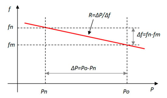
Figure 5.
EPS frequency droop control.
The derivative module emulates conventional generating units’ inherent property to support the grid frequency regulation, based on Equation (1). It is possible to consider the whole system or its part (one control area) and introduce ωCOI:
where ΔωCOI is the rotational speed deviation of the COI from the nominal synchronous speed:
The wind power injected in the EPS is contained in Pe [30] according to:
The controller provides an active power injection proportional to the derivative of the COI frequency of the control area in which WPP is connected, described by:
where derivative gain Kd acts as synthetic inertial constant, increasing the total system inertia.
The derivative of the COI frequency deviation is calculated according to:
As a result, the frequency derivative effect has the same nature as the synchronous generators’ inertia in the selected control area. When the frequency decreases, active power injection increases due to the negative derivative of frequency. It continues to change until the frequency variation becomes zero. Due to practical implementation, active power injection should be limited, and limitation band ±ΔPdmax band is introduced. Wind generator (REGCAU1) and wind electrical (REECAU1) models are controlled by the wind auxiliary control model’s output reference signal (Pref).
Having in the mind ongoing marketization of EPS inertial service, the proposed scheme can also be applied to selected generators belonging to balance responsible parties (BRPs). BRPs are financially responsible for continuously maintaining the balance between supply and demand within their generation portfolio.
5. EPS Modelling and Simulations
Traditionally, the generation’s portfolio in EPS of this Southeast Europe region is based mainly on hydro and thermal power plants. The transmission network of these countries operates at 400 kV, 220 kV and 110 kV voltage levels. The high voltage network through the region is well meshed, providing robust interconnections illustrated in Figure 6. The nominal transmission capacity of interconnectors on average is above 40% of the regional average peak load. Some countries like BIH and Croatia have an unusually high capacity of interconnectors regarding their peak load.
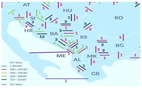
Figure 6.
Southeast Europe (SEE) Region Electric Power System.
The SEE region’s power system, presented in Figure 6, is modelled using PSS/E software. The PSS/E consists of a complete set of programs for the study of the EPS with both steady-state and dynamic simulations. The PSS/E software interfaced with Python programming language with the application program interface (API) is used to perform the dynamic simulations [31]. There are two automation processes in the PSS/E based on the API: the Python interpreter (Python) and the IPLAN simulator. Python has great flexibility in operation and has predefined modules for interacting with PSS/E [32]. In this paper, frequency response metrics, frequency of COI calculations and plots are performed with Python scripts.
The EPSs of Slovenia (SI), Croatia (HR), Bosnia and Herzegovina (BIH), Serbia (RS), North Macedonia, Kosovo, and Montenegro are modelled in detail, using complete models of generators, excitation systems and governors. The PSS/E library includes a family of generator models. GENROU (round rotor generator model) and IEEEG1 governor model is used to present thermal units [33]. IEEEG1 is the IEEE recommended general model for steam turbine speed governing systems. The hydro generators are presented with GENSAL (salient pole generator model) with HYGOV turbine speed governing systems. The simplified excitation system’s dynamic model SEXS is used for all types of synchronous generators.
The classical generator model (GENCLS) is used to present all generators in EPSs of Hungary, Romania, Bulgaria, Albania, Greece, and Turkey. GENCLS is the classical constant voltage behind the transient reactance generator model (with H = 4 s, D = 0.5 p.u.).
The EPS is assumed to be working in a steady-state equilibrium before the active power disturbance’s initialization. The simulated steady-state, network topology, generation units schedule and loads corresponding to the real scenario are recorded on 16 February 2020. Data are obtained from the ENTSO-E transparency platform. The total power generation in the analyzed system is 84.3 GW and consists of thermal and hydro as well as some wind power plants. The total system load is 82.6 GW. The FR analysis of each control area is out of the scope of this paper. This paper is focused on the FR performance of the ENTSO-E SCB control block (Slovenia, Croatia and BIH).
The power system data of ENTSO-E control block Slovenia, Croatia and BIH used in simulations are presented in Table 4.
Table 4.
ENTSO-E Slovenia, Croatia and BIH (SCB) control block electric power system (EPS) data.
The aggregated wind turbine model is used to represent all wind turbines inside a wind farm. The wind speed remains constant during simulation. The user-written auxiliary model FCPCAU1 is used to simulate WTGs in BIH EPS. There are two WPPs connected in the BIH control area, WPP Jelovaca (18 × 2 MW) and WPP Mesihovina (22 × 2.3 MW). The values of the parameters of the FCPCAU1 are provided in Table 5.
Table 5.
FCPCAU1 parameter values.
5.1. Southeast Europe Region EPS Frequency Response Simulation
The active power disturbance ΔPL = 2.75 (p.u.), sudden loss of production of TPP Stanari (275 MW) in the BIH control area, is applied at t = 2 s after the simulation start. Based on imported data from PSS/E time-domain simulations, Python scripts have been developed to automate calculations and plots of EPS frequency response. For the simulated disturbance, the COI frequency is calculated for the SCB control block and the entire SEE region.
Power system frequency responses of Slovenia, Croatia, BIH and of FCOI of SEE region are presented in Figure 7.
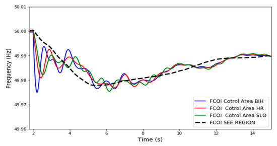
Figure 7.
EPS frequency response, simulation time 15 s.
Following the disturbance, frequency excursions of COI Slovenia, Croatia and BIH are different and experienced inter-area electromechanical oscillations (EMOs).
These low frequency (0.1–0.8 Hz) EMOs are associated with coherent groups of synchronous generators from each control area (EPS) swinging against the other coherent groups of synchronous generators. Each coherent group oscillates differently than the others. In particular, at a given time, some groups locally accelerate, and others locally decelerate. Frequency oscillations caused by the active power imbalance are damped, and after 10–15 s, the system obtains a new steady-state.
At the end of the simulation (Figure 7), the system will not return to the nominal frequency (50 Hz) on its own. To compensate for the remaining frequency deviation, ENTSO-E Continental Europe interconnected system uses automatic secondary frequency control called automatic generation control (AGC). The AGC is not included in this simulation model.
5.2. Southeast Europe Region Frequency Response Evaluation
The frequency response (FR) performance indicators and inertia concentration are calculated for individual control areas and the entire SEE region. The results are presented in Table 6. The steady-state frequency deviation Δfss is the frequency deviation from the rated (nominal) system frequency (50 Hz) in a new steady-state, while Δfmax is the highest absolute frequency deviation (nadir). Generally, after the applied disturbance, the calculated frequency response metrics show that the system frequency remains in the prescribed range.
Table 6.
Frequency response metrics of COI of control areas, SEE Region and WPP Jelovaca 110 kV PCC.
The lowest point of frequency drop (nadir) is recorded in EPS of BIH (49.9749 Hz) and the time it takes to reach the nadir tmin = 0.22 (s) (immediately after a disturbance occurred). The frequency decline of the SEE region is stopped at tmin = 5.38 (s) (3.38 s after a disturbance occurred) at a frequency value of 49.9778 Hz. The final steady-state frequency deviation in the SEE region EPS is Δfss = 10 (mHz).
Deviations from nominal frequency by more than 20 mHz are corrected by activating individual generators’ primary frequency regulators and, if necessary, by activating the energy for frequency restore reserve FRR [34]. FRR is an operating reserve activated to restore frequency to the nominal value and power flows on the interconnected lines to the pre-fault scheduled values. It is also used for secondary and tertiary regulation. In Figure 8, the FCOI of SEE region, frequency measured at PCC of WPP Jelovaca and FCOI of EPS BIH are presented. The frequency at PCC of WPP Jelovaca (red line) is obtained from time-domain simulation, computing the numerical derivative of the bus voltage phase angle. It is evident that in the initial phase, the local bus frequency (red line) is much closer to the frequency of the total system frequency of the SEE region (black dotted line) than the frequency of COI BIH (blue line). It can be concluded that the frequency representation using the measured generator speeds (e.g., FCOI of the control area) more closely reflects the frequency dynamics of a local EPS.
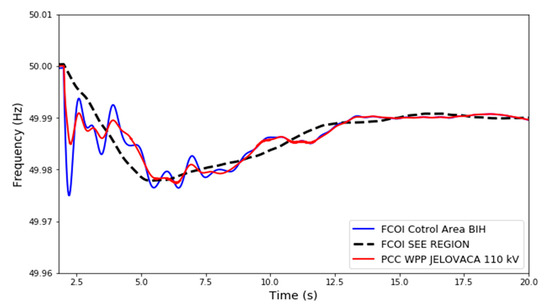
Figure 8.
EPS frequency response, time simulation 20 s.
The initial slopes (ROCOF) of each control area and SEE region are presented in Figure 9. As expected, recorded ROCOFs of COI of Slovenia and Croatia are lower than the COI of BIH.
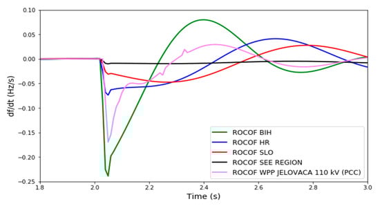
Figure 9.
ROCOF of EPS.
Following the disturbance, the maximum ROCOF of COI BIH (−0.238 Hz/s) is significantly higher than the ROCOF of local frequency at PCC of WPP Jelovaca (−0.169 Hz/s). This different frequency behavior is used to design wind inertial controller FCPCAU1 based on specifics of the FCOI of a control area. The performed simulation and calculations show that EPS of BIH, which is a significant exporter, has the largest inertia concentration 6.7 (s), due to low total system load and numerous synchronous generators connected to the grid. The inertia concentration of the EPS of Croatia is the smallest 3.8 (s) in the SCB LFC block. Croatia is a regional importer of electricity and its total load (2.100 MW) is high relative to the local generation (1.680 MW) and the number of connected SGs. The concentration of inertia indicates a potential need for WPPs located in EPS of Croatia to participate in the inertial response. It is an important finding because the EPS of Croatia has the largest installed wind capacity and the smallest kinetic energy in the SCB LFC block (Table 4).
5.3. WPP Inertial Controller FCPCAU1 Performance
Based on previous findings and calculated FR indicators, the WPPs’ inertial contribution highly depends on used frequency input signals. In Figure 10, the power output of WPP Jelovaca (blue dotted line) during the analyzed disturbance is presented. When the frequency drop is detected (red line), the inertial controller FCPCAU1 continuously follows dfCOI/dt and forces the WPP to generate additional power. The additional power output from synthetic inertia depends on ROCOF, WPP inertia constant and WPP Pmax. In the initial phase of active power response, WPP Jelovaca additionally generates 0.4 MW.
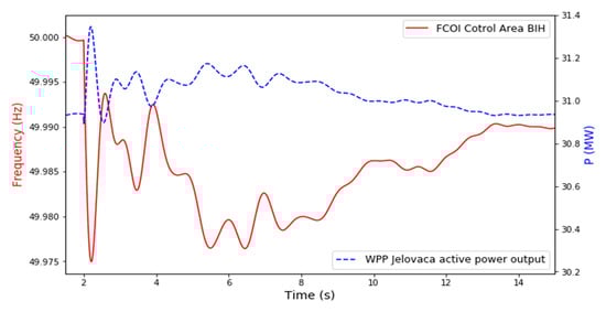
Figure 10.
WPP Jelovaca (BIH) active power response.
In Figure 11, a comparison between WT active power responses considering different input signals for synthetic inertia control is presented. The initial peak of the inertial response triggered by the FCOI of the BIH control area (red line) results from fast releasing kinetic energy from WT. It is more significant than when local frequency measured at PCC of WPP (blue dotted line) is used.
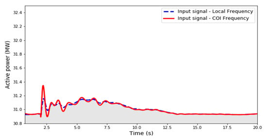
Figure 11.
WPP Jelovaca (BIH) active power response comparison.
The value of derivative gain Kd highly influences FCPCAU1 performance. Gain (Kd) excessive value could lead to WT rotor speed instability, because Kd scales change at every frequency. The inertial controller’s parameters should be carefully determined to avoid eventual dangerous consequences on WT’s mechanical parts.
In Figure 12, the FCOI of SEE region, FCOI of control area Croatia and frequency obtained from PSS/E simulation at PCC of WPP Ponikve (34 MW), WPP Velika Glava (43 MW) and WPP Vratarusa (42 MW) are presented. These wind farms are connected to the 110 kV transmission grid of the Croatia control area. WPP Ponikve and Velika Glava are electrically close to hydropower plants (HPP Dubrovnik and HPP Orlovac), so the frequency excursion at their PCC is significantly influenced by these HPP. WPP Vrataruša is electrically more distant from the fault location, so the frequency change at PCC is slightly different.
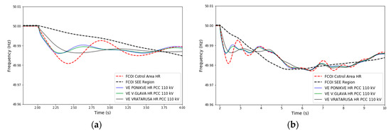
Figure 12.
EPS frequency response. (a) simulation time 4 s, (b) simulation time 10 s.
In the first few seconds, the dynamics of the Croatian FCOI better characterizes the nature of the imbalance than the local PCC frequency at WPP Vratarusa. The frequency response indicates that the system frequency excursion in the inertial phase of disturbance is not the same in all system nodes. This finding will result in different synthetic inertial responses depending on the wind power plant (WPP) locations. Using FCOI of a control area instead of local frequency, all WPPs can provide a “firm frequency response” within the first few seconds after the disturbance, regardless of their locations.
6. Conclusions
The wind is expected to be a significant new electricity generation source in Southeast Europe, but WPP integration is slow and their share in total production is small. Generally, the frequency stability and control of EPS in this region are still based on the dynamic characteristics and controllability of conventional power plants.
Simulation results show that the modelling and the frequency calculation (COI or local frequency) significantly differ in a power system’s transient behavior with high WPP integration. A new FR indicator, “concentration of inertia”, was introduced. This indicator shows how inertia is distributed in real interconnected systems and can be relevant for the inertial response service’s upcoming marketization. The inertial response of WT based on the COI frequency shows that WTTs can provide a “firm frequency response” in the first few seconds after the disturbance, regardless of their location. Some essential points like the impact of noise, time delay and measurement data quality on the estimation COI signal still require further research to enhance the WT inertial response based on the control area FCOI. In the future (low inertia) EPS, frequency control methods need to be redefined and new schemes need to be developed. The authors believe that this work presents a small step in that direction.
Author Contributions
Conceptualization, A.M. and M.K.; software, A.M. and E.N.; validation, A.M. and E.N.; formal analysis, A.M.; simulations, A.M.; writing—original draft preparation, A.M.; writing—review and editing, A.M., M.K. and E.N.; visualization, A.M.; supervision, M.K. All authors have read and agreed to the published version of the manuscript.
Funding
This research received no external funding.
Conflicts of Interest
The authors declare no conflict of interest.
References
- Ulbig, A.; Borsche, T.S.; Andersson, G. Impact of Low Rotational Inertia on Power System Stability and Operation. IFAC 2014, 47, 7290–7297. [Google Scholar] [CrossRef]
- Wind Europe. Wind energy in Europe in 2019—Trends and statistics. February 2020. Available online: https://windeurope.org/wp-content/uploads/files/about-wind/statistics/WindEurope-Annual-Statistics-2019.pdf (accessed on 1 September 2020).
- Lalor, G.; Mullane, A.; O’Malley, M. Freq. control and wind turbine technologies. IEEE Trans. Power Syst. 2005, 20, 1905–1913. [Google Scholar] [CrossRef]
- Doherty, R.; Mullane, A.; Nolan, G.; Burke, D.J.; Bryson, A.; O’Malley, M. An Assessment of the Impact of Wind Generation on System Frequency Control. IEEE Trans. Power Syst. 2010, 25, 452–460. [Google Scholar] [CrossRef]
- Muljadi, E.; Gevorgian, V.; Singh, M.; Santoso, S. Understanding Inertial and Frequency Response of Wind Power Plants. In Proceedings of the 2012 IEEE Power Electronics and Machines in Wind Applications, Denver, CO, USA, 16–18 July 2012. [Google Scholar]
- Nguyen, H.T.; Yang, G.; Nielsen, A.H.; Jensen, P.H. Challenges and Research Opportunities of Frequency Control in Low Inertia Systems. In Proceedings of the 2nd International Conference on Electrical Engineering and Green Energy, Rome, Italy, 28–30 June 2019. [Google Scholar]
- Milano, F.; Darfier, F.; Hug, G.; Hill, D.J.; Verbic, G. Foundations and Challenges of Low-Inertia Systems; IEEE: Piscataway, NJ, USA, 2018; pp. 1–25. [Google Scholar]
- Gonzalez-Longatt, F.M. Impact of emulated inertia from wind power on under-frequency protection schemes of future power systems. J. Mod. Power Syst. Clean Energy 2016, 4, 211–218. [Google Scholar] [CrossRef]
- AEMO. Black system South Australia 28 September 2016; Technical Report; Australian Energy Market Operator Limited: Sydney, Australia, 2017. [Google Scholar]
- OFGEM. Technical Report on the Event of 9 August 2019; OFGEM: Canary Wharf, UK, 2019.
- Tielens, T.; Hertem, D.V. The relevance of inertia in power systems. Renew. Sustain. Energy Rev. 2016, 55, 999–1009. [Google Scholar] [CrossRef]
- Bevrani, H.; Ise, T.; Miura, Y. Virtual synchronous generators: A survey and new perspectives. Int. J. Electr. Power Energy Syst. 2014, 54, 244–254. [Google Scholar] [CrossRef]
- Heydari, R.; Savaghebi, M.; Blaabjerg, F. Fast Frequency Control of Low-Inertia Hybrid Grid Utilizing Extended Virtual Synchronous Machine. In Proceedings of the 11th Power Electronics, Drive Systems, and Technologies Conference (PEDSTC), Tehran, Iran, 4–6 February 2020; pp. 1–5. [Google Scholar]
- Wu, Z.; Gao, W.; Gao, T.; Ya, W.; Zhang, H.; Yan, S.; Wang, X. State-of-the-Art Review on the Frequency Response of Wind Power Plants in Power Systems; Springer: Berlin/Heidelberg, Germany, 2017. [Google Scholar]
- Osmic, J.; Kusljugic, M.; Mujcinagic, A. Fuzzy Logic Controller for Inertial Support of Variable Speed Wind Generator. In Proceedings of the Medpower-10th Mediterranean Conference on Power Generation, Transmission, Distribution and Energy Conversion, Belgrade, Serbia, 6–9 November 2016. [Google Scholar]
- Díaz-González, F.; Hau, M.; Sumper, A.; Gomis-Bellmunt, O. Participation of wind power plants in system frequency control: Review of grid code requirements and control methods. Renew. Sustain. Energy Rev. 2014, 34, 551–564. [Google Scholar] [CrossRef]
- Eriksson, R.; Modig, N.; Elkington, K. Synthetic inertia versus fast frequency response: A definition. IET Renew. Power Gener. 2018, 12, 507–514. [Google Scholar] [CrossRef]
- Gonzalez-Longatt, F.M. Activation Schemes of Synthetic Inertia Controller on Full Converter Wind Turbine (Type 4). In Proceedings of the IEEE Power & Energy Society General Meeting, Denver, CO, USA, 26–30 July 2015. [Google Scholar]
- Mujcinagic, A.; Kusljugic, M.; Osmic, J. Frequency Response Metrics of an Interconnected Power System. In Proceedings of the 54th International Universities Power Engineering Conference (UPEC), Bucharest, Romania, 3–6 September 2019. [Google Scholar]
- Agathokleous, C.; Ehnberg, J. A Quantitative Study on the Requirement for Additional Inertia in the European Power System until 2050 and the Potential Role of Wind Power. Energies 2020, 13, 2309. [Google Scholar] [CrossRef]
- Thiesen, H.; Jauch, C.; Gloe, A. Design of a System Substituting Today’s Inherent Inertia in the European Continental Synchronous Area. Energies 2016, 9, 582. [Google Scholar] [CrossRef]
- Milano, F. Rotor Speed-Free Estimation of the Frequency of the Center of Inertia. IEEE Trans. Power Syst. 2018, 33, 1153–1155. [Google Scholar] [CrossRef]
- ENTSO-E. Network Code on Load-Frequency Control and Reserves. 2013. Available online: https://eepublicdownloads.entsoe.eu/clean-documents/pre2015/resources/LCFR/130628-NC_LFCR-Issue1.pdf (accessed on 5 September 2020).
- Grainger, J.J.; Stevenson, W.D. Power System Analysis; McGraw-Hill: New York, NY, USA, 1994. [Google Scholar]
- ENTSO-E. Nordic Report Future System Inertia V2. 2018. Available online: https://docs.entsoe.eu/id/dataset/nordic-report-future-system-inertia/resource/6efce80b-2d87-48c0-b1fe-41b70f2e54e4 (accessed on 5 September 2020).
- Anderson, P.; Fouad, M.A. Power System Control and Stability; John Willey & Sons: Hoboken, NJ, USA, 2003. [Google Scholar]
- Kovaltchouk, T.; Debusschere, V.; Seddik, B.; Fiacchini, M.; Alamir, M. Assessment of the Impact of Frequency Containment Control and Synthetic Inertia on Intermittent Energies Generators Integration. In Proceedings of the Eleventh International Conference on Ecological Vehicles and Renewable Energies (EVER), Monte Carlo, Monaco, 6–8 April 2016. [Google Scholar]
- González Rodriguez, A.G.; González Rodriguez, A.; Burgos Payán, M. Estimating wind turbines mechanical constants. Renew. Energy Power Qual. J. 2007, 1, 697–704. [Google Scholar] [CrossRef]
- Krishnat, P.; Jay, S. Creating Dynamics User Model Dynamic Linked Library (DLL) for Various PSS®E Versions; Siemens Energy Inc.: Erlangen, Germany, 2012. [Google Scholar]
- Rodríguez-Bobada, F.; Ledesma, P.; Martínez, S.; Coronado, L.; Prieto, E. Simplified wind generator model for Transmission System Operator planning studies. In Proceedings of the 7th International Workshop on Large Scale Integration of Wind Power and on Transmission Networks for Offshore Wind Farms, Madrid, Spain, 26–27 May 2008. [Google Scholar]
- SIEMENS. Siemens PTI.PSS/E 34 Application Program Interface (API); SIEMENS: New York, NY, USA, 2015. [Google Scholar]
- Khalid, M.U. Python Based Power System Automation in PSS/E; Lulu Enterprises, Inc.: Morrisville, NC, USA, 2014. [Google Scholar]
- SIEMENS. Siemens PTI.PSS/E 34 Model Library; SIEMENS: New York, NY, USA, 2015. [Google Scholar]
- Independent System Operator in BIH, Grid Code. January 2019. Available online: https://www.nosbih.ba/files/dokumenti/Legislativa/Mrezni%20kodeks/EN/GRID%20CODE%20%20January%202019.pdf (accessed on 18 September 2020).


Publisher’s Note: MDPI stays neutral with regard to jurisdictional claims in published maps and institutional affiliations. |
© 2020 by the authors. Licensee MDPI, Basel, Switzerland. This article is an open access article distributed under the terms and conditions of the Creative Commons Attribution (CC BY) license (http://creativecommons.org/licenses/by/4.0/).