Article

Real-Time 3D Printing Remote Defect Detection (Stringing) with Computer Vision and Artificial Intelligence

by
Konstantinos Paraskevoudis
,
Panagiotis Karayannis
and
Elias P. Koumoulos
*
IRES—Innovation in Research & Engineering Solutions, Rue Koningin Astritlaan 59B, 1780 Wemmel, Belgium
*
Author to whom correspondence should be addressed.
Processes 2020, 8(11), 1464; https://doi.org/10.3390/pr8111464
Submission received: 15 October 2020 / Revised: 8 November 2020 / Accepted: 12 November 2020 / Published: 16 November 2020
(This article belongs to the Section Process Control and Monitoring)

Abstract

:
This work describes a novel methodology for the quality assessment of a Fused Filament Fabrication (FFF) 3D printing object during the printing process through AI-based Computer Vision. Specifically, Neural Networks are developed for identifying 3D printing defects during the printing process by analyzing video captured from the process. Defects are likely to occur in 3D printed objects during the printing process, with one of them being stringing; they are mostly correlated to one of the printing parameters or the object’s geometries. The defect stringing can be on a large scale and is usually located in visible parts of the object by a capturing camera. In this case, an AI model (Deep Convolutional Neural Network) was trained on images where the stringing issue is clearly displayed and deployed in a live environment to make detections and predictions on a video camera feed. In this work, we present a methodology for developing and deploying deep neural networks for the recognition of stringing. The trained model can be successfully deployed (with appropriate assembly of required hardware such as microprocessors and a camera) on a live environment. Stringing can be then recognized in line with fast speed and classification accuracy. Furthermore, this approach can be further developed in order to make adjustments to the printing process. Via this, the proposed approach can either terminate the printing process or correct parameters which are related to the identified defect.

1. Introduction

1.1. Computer Vision and Object Detection

Computer Vision is considered an interdisciplinary field of informatics, mathematics and image processing, which aims to develop techniques and algorithms so that computers can process, interpret and understand visual information such as video and image. Initial research in Computer Vision in the 1960s aimed to develop computer algorithms which could mimic the human visual behavior [1]. In the next years, a research boost is remarkable, where algorithms do not only try to copy the human eye perception but also improve themselves by constantly dealing with new data. Based on this principle, newly Artificial Intelligence applications on Computer Vision were described. In medicine and healthcare, computers have been trained to recognize vital image features from image data such as Magnetic Resonance Imaging (MRI) for patient status detection and diagnosis [2,3]. Computer Vision also has a variety of applications in industry, where algorithms aid in controlling processes serving automation, inspection, etc. [4,5]. Autonomous vehicles are also a widely known application of Computer Vision [6]. In the field of commercial monitoring, Computer Vision and Artificial Intelligence has been used for the detection of events such as real-time people counting [7] or as a human–computer interaction tool.

1.2. Applications on Additive Manufacturing

Computer Vision has been applied on laser powder bed additive manufacturing for the automated detection and classification of anomalies and unwanted phenomena that can appear during the powder spreading stage [8]. Specifically, a machine learning model was trained on anomaly-related image data and deployed for live monitoring and analysis of powder bed images, serving as a real-time control system attached to the machine used [8]. Additionally, Convolutional Neural Networks have been trained in order to detect delamination and splatter defects in the additive manufacturing of metal components with laser-powder bed fusion [9]. The aforementioned approach achieved a classification accuracy of 96.8%. Convolutional Neural Networks have also been used as a quality inspection tool for the recognition of cracks, gas porosity, and lack of fusion in metal additive manufacturing with an accuracy of 92.1% [10]. Another study revealed the capabilities of residual neural networks (ResNet) in the detection of defects in fused deposition modeling (FDM). In this approach, the trained neural network was able to predict on a live 3D printing environment the delamination and warping defects from analyzing images of the printer’s parts [11]. In this, the detection was not decided from the printed object’s shape but from the printers’ setup configuration and the prior knowledge on its correlations with defects. Thus, the trained model detected the nozzle height from images of the printing head and correlated the detected height with actual defect probabilities.
In the field of fused filament fabrication, Computer Vision has been also used for the automated quality assessment of products. A real-time algorithm which reconstructs the 3D printed model from the final printed objects and compares differences was able to achieve 100% detection rate for failures [12]. Via this, phenomena such as clogged nozzle and loss of filament were being identified. Additionally, the proposed algorithm was further developed in order to stop the printing process when the respective errors between reconstructed shape and STL file exceeded 5%. This detailed comparison between 3d printing model and the printed shape has low cost requirements and has shown promising results at detecting effectively clogged nozzle, loss of filament, or an incomplete project for a wide range of 3D object geometries and filament colors and can also be with automated decision making based on detections [12,13]. However, such an approach considers major and obvious macro-level defects, while its capability of detecting small-scale defects is usually not evident. In addition, the computation of the image processing steps for the defect identification is proved consuming in terms of time requirements, which can be problematic for some cases, where the defect needs to be identified almost instantaneously. A considerable aspect in developing a method for 3D printing error detection is that the major and catastrophic print errors, such as loss of filament may be considered more compatible to being identified at the source (e.g., by a filament sensor), rather than through their effects on the object being printed. This appears due to the fact that conventional sensor techniques can be adapted to address these issues, while this seems significantly more challenging for smaller-scale defects or object and print process-centered defects, necessitating the use of a technique such as Computer Vision for proper identification. As reported in the 3D printing community, there are various recommendations on how to apply a filament sensor to popular 3D printer devices [14], while some high-end printers may feature a filament sensor as an add on (e.g., 3D Gigabot 3D printers [15]). Image processing and Computer-Vision-based approaches may be more useful for the 3D printer user when they are designed to detect errors that are integrally connected to the print process and cases where the source of the issue is only identifiable through its effect (e.g., warping, stringing, and over/under-extrusion). This process can provide insights into potential issues of the print parameter setup that could be difficult to predict due to level of experience of user or when testing novel/unique materials. Another approach combined conventional image processing techniques in order to analyze a printed object layer by layer and then apply corrections to the printing process given a set of decision rules [13]. This approach is using a camera, which allows for the observation of both the active printable layer and part of the printing model from the side. Thus, by combining the camera input and G-Code trajectories for a given layer, it is possible to analyze the visibility of the side area of the printed part. With this approach, defects such as blocked nozzle, lack of material and major deformations can be detected. A second technique tracks significant horizontal and vertical displacements of the printed part based on the binary layer template obtained from the G-Code trajectories and determines fine rotation and translation within the small deviation range. Via this, possible mismatches between the real outline and the reference borders are identified. This technique is used for the identification of defects such as missing layers, dimensional inaccuracies, print not sticking to bed and print bending. Finally, a third technique based on Local texture analysis handles irregular sections of the texture within the layer infill: a combination of convolutional stages on the image and unsupervised machine learning (Gaussian Mixture Model clustering) is applied for segmenting the textures. This approach can identify infill-related defects such as weak or under-extruded infill, deformed or incomplete infill and gaps between infill and shell. Despite being able to identify multiple defects, and being applicable to errors of various scales, addressing the method compatibility issues discussed, this approach is slow, as the average computational time is 21.4 s. In addition, there is a demand on printer calibration and configuration prior to application, and the failure detection ability of the approach depends on the resolution of the camera, the distance to the print area, and the size of the part. In this approach, the print errors were connected with error-specific corrective actions, which is a crucial feature that enhances the practicality of the approach. While a large library of detectable and addressable errors is highly valuable, it is possible that the same prediction confidence and efficiency may not be achieved for all classes of errors. This may be attributed to the wide variety in the nature of the deformations that each defect produces on the object being printed, introducing difficulties in their identification through an integrated approach. A case-by-case error detection approach could assist in identifying refinements for more efficient identification of classes of errors. This would require repeated prints of known introduced defects and the testing of the system for each class, leading to gaps being identified and refinements being developed for each error identifying “module”. Applications of layer-wise analysis can intervene to the printing parameters and either stop the process or adjust it in such a way, where the identified printing failures are being corrected. Such systems can help save time and material [12,13]. However, the use of deep learning techniques for the recognition of such failures can be more accurate [16]. Experimentation on different angles can also help increase detection rates when comparing the original computer-aided design (CAD) model to a reconstructed layer shape [13,16]. However, adding multiple angles as a requirement for the camera input increases the degrees of freedom and makes the application of the approach on different environments (3D printer, etc.) more difficult. Clogged nozzle, object not sticking to bed, extruder blobs, warping and over/under extrusion are printing failures that have also been examined: a detailed comparison of printed layers and the original 3D model with image segmentation and masking techniques was capable of identifying the above [14]. The first step of this approach is to take an input image capture from a camera of the first layer when it is printed. In addition, a digital model is created by simulating the first layer from the G-code. The snapshot of the real print (first layer) and the digital model are given as input to a deviation detection algorithm. Both images are processed with Image segmentation algorithms (Thresholding and Masking) to remove background noise. After these steps, both images display only black and white pixels. Finally, the Douglas–Peucker algorithm is applied in order to create contours on each image. The resulted contours are compared and a deviation between the two is extracted. The proposed methodology shows no generalization in other cases and lacks information regarding runtime and computational requirements. In addition, manual calibration and configuration of the printer and the camera position is required.
Popular image processing libraries such as OpenCV [17] have also been used in applications of Computer Vision in 3D printing [16,18]. The failures of detachment from print bed, not continuous material flow from nozzle and printed object deformation have been detected with blob detection, which refers to the identification of regions in a given image with high variation in brightness compared to all other regions [18]. Combined with image thresholding at the color value of the printed filament, the aforementioned approach was developed as a software which serves as an error detection system for FDM 3D printers [18]. Image thresholding requires one or more parameters; this results in an increase in the degrees of freedom. However, the aforementioned approach asks for user input through a User Interface in order to automatically determine the required parameters as a first step. The threshold parameters are user selected for every printed object and therefore not subjective to algorithmic selection. Then, the red-green-blue color model (RGB) video frames are converted to hue-saturation-value color model (HSV). The image is then cropped automatically: an algorithm determines the print-bed upper surface by finding associated parallel lines in a defined distance to a virtual line between the visual markers for the print bed. The visual markers must be places prior to application. Then, image thresholding (on selected parameter of first step) is applied. A blob detection algorithm on the binary image is finally used to identify the defects. This approach capable of a 60 to 80 percent detection rate for failure detection with a false positive detection rate of 60 to 80 percent. However, it is rather case specific and the calibration of multiple parameters (camera position, visual markers) is needed in order to be effectively applied. In addition, the video resolution of the use case is 640 × 480 pixels, influencing computational effort requirements. This resolution was considered adequate for the objectives of the study, but may be limited in expanding the methodology, or if higher certainty would be required in identifying the errors. The approach has also been identified as sensitive to producing false results due to lighting changes. It is quite important to note that approaches that prioritize cost-effectiveness are reasonably expected to be of the highest value to non-expert 3D printing users. Such users are most likely to be inhibited by additional requirements of the process such as precise camera positioning and calibration, presenting barriers in the reproducibility of the method. It seems conceptually valid to couple the more expensive methods equipment-wise with more demanding monitoring setups, while keeping a simple monitoring configuration for the cost-effective methods, with an expected compromise in detection capabilities or accuracy.
Additionally, warping has also been identified with application of blob detection and image segmentation techniques in capture images from the printing object and a comparison to the original 3D model [19]. A layer-wise approach is using a color camera to capture an image of the object after each new layer is added [19]. Using the workpiece CAD model, and perspective projection, an expected image of the object geometry is rendered for each of the captured images. A differential imaging algorithm compares these two images and determines the existence of a defect based on the simulation of what the object under print should look like for any given moment in time. The above methodology can be used for the early detection of warping, build plate delamination and extrusion failure, while the study of the error signal as a function of printed layer number can assist in determining the time point of print failure. For complicated print shapes, this feature can be highly valuable in defining areas of focus to refine print parameters, make localized changes (e.g., variable layer height) in the layer print parameters on the area of failure, or provide insights into how to potentially revise the object design. Despite the simplistic setup, which is encouraging for a typical non-expert 3D printer user, the approach requires that camera parameters need to be estimated beforehand. In addition, no accuracy metrics and generalization tests are given and the three failure modes cannot be distinguished based on the method implemented, presenting barriers in identifying the root cause of print issues. Typically, image processing approaches for error detection requires calibration of the used camera and printer [12,13,18,19]. This is the most common challenge and bottleneck in the field of the automated detection of 3D printing defects, as it significantly increases the degrees of freedom and the actions required from the user. Most existing research relies on conventional image processing techniques. On the other hand, learning-based algorithms have a promising potential in identifying errors, failures and defects in 3D printing while keeping user interaction to a minimum. A proposed machine learning algorithm was able to detect collisions in the 3D printing [20]. In Table 1, the pros and cons of existing applications and techniques are summarized below in Table 1.

1.3. Common Defects in 3D printing

For the vast majority of Fused Filament Fabrication (FFF) 3D printer devices, sensors and feedback controls are only featured for the temperature of the nozzle and build platform. Functional check sensors may be present for a number of operational prerequisites, such as filament detection. Typically, commercial FFF 3D printers do not conduct monitoring of the printing process or any check if printing proceeds as expected. The formation of defects, or even critical failures, such as the print object losing adhesion to the print bed will not stop the print process, and printing will continue if not interrupted by the operator, leading to waste of material, power, effective equipment operation time, as well as potentially causing malfunctions to printing parts (e.g., nozzle clogging). This leads to process operators needing to systematically check print progress. Continuous monitoring of the printing process may be implementable by operators of one printer but can be impractical in larger-scale settings where multiple printers are operating simultaneously. Prolonged presence of operators in the close proximity of printers in function should be minimized for safety-related reasons as well, in order to diminish exposure to ultrafine particles and Volatile Organic Compounds, to the highest extent reasonably applicable [21]. The inconvenience of constant supervision of 3D printing processes can be partially alleviated by simple remote supervision. To this end, several commercial 3D printers possess built-in camera features, and the placement of external video cameras to observe print progress is quite common. The open source OctoPrint software [22] can be used for printer remote control and monitoring in supported devices. However, user attendance to the video is required in systematic intervals, which can be problematic, particularly in multiple printer operation cases.
To the authors’ best knowledge, structuring a defect detection method around identifying a specific defect has not been extensively explored, with the literature favoring approaches that target monitoring deformation and deviation of the 3D printed object, leading to identification of major defects or detecting that one out of a group of possible defects has occurred. We therefore suggest that an array of defect-specific detection methods could potentially serve as elements of a more integrated approach. In this work, we investigate the automated recognition of a common defect of any 3D printing process, called stringing. Stringing (also known as oozing) describes a phenomenon where small or tiny strings of the printed plastic remain on the surface of the printed object and cause an aesthetic failure, which could also affect the mechanical properties of the object. Such defects may also require the object to be post-processed for the unwanted strings removal, and thus investment of working time, which is a minor inconvenience for home-use prints, but would be a significant issue in larger batch production cases. This phenomenon happens when extruded plastic is held out of the nozzle while the extruder is moving. Stringing has known origin causes, varying from high temperatures to high printing speeds or misconfiguration in retraction settings (filament “pulled back” through the hot end by the extruder motor when not in area for deposition). Stringing can also cause slight dimensional distortion of the object, especially in smaller objects. The string being formed may generate small protrusions in each end (as shown in Figure 1 below), which may be quite a critical issue for applications where dimensional fidelity is paramount. Additionally, optimal print parameters are not universal for all materials, specific geometries or intended final object properties. This requires, before effectively using a newly applied material for manufacturing on a large scale, a distinct portion of work to be allocated for identifying functional printing parameters. Time investment and potential complications are increased for using non-commercial (e.g., recycled), or specialty/novel materials (e.g., nanomaterial-enabled filaments). Techniques for the minimization of time, resources and human involvement required for this adaptation phase can prove quite useful to the manufacturing field.

2. Methodology

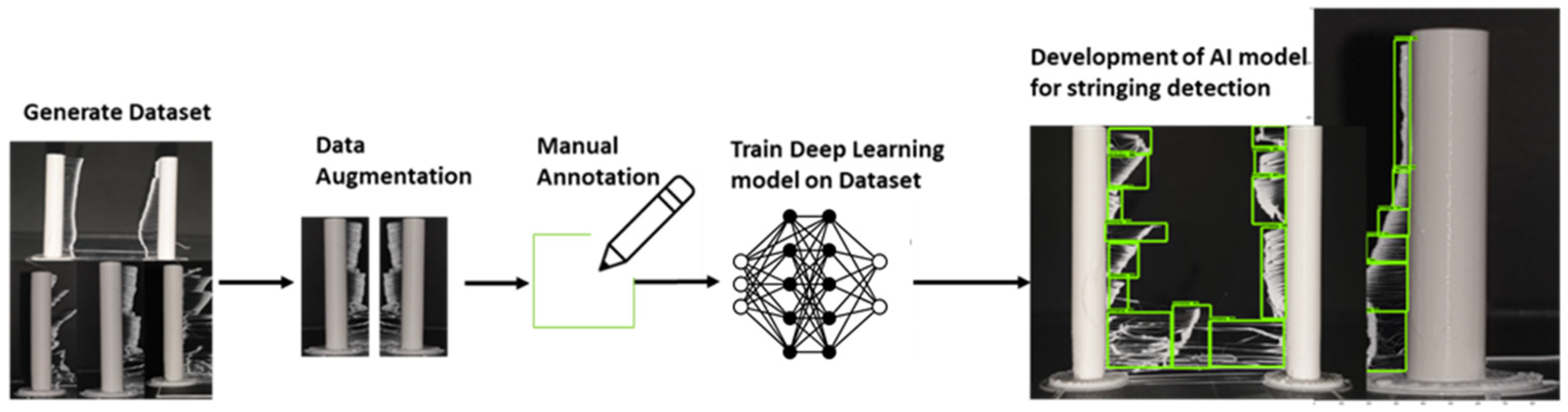
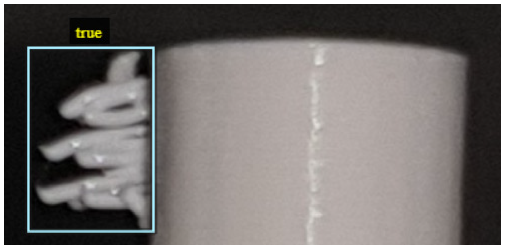
2.1. Data Collection and Annotation

The 3D printer Prusa i3 MK3S was used for the collection of images of printed objects with defects. A simple “Stringing test” object was designed and used for the generation of the images. Specifically, major defects were introduced via the known related printing parameters. A final Dataset of 500 images with a stringing phenomenon was collected as a training Dataset for the Single Shot Detector (Deep Neural Network). After collecting training data for the stringing defect, various Data Augmentation techniques were applied in order to raise the amount of training instances. Data Augmentation is a set of techniques which are applied to existing datasets and create new synthetic data with meaningful information [23], and here was deemed necessary. Specifically, for each image on the base training set, we applied scaling to half the size (image resize), horizontal flipping, cropping (randomly), 90 degrees rotation and brightness change (randomly). Applying these 5 data augmentation techniques to each of the 500 original training images, we obtained a final dataset of 2500 images.
In order to train any model on the image features, the ground truth (the true classes within an image as well as their location in the image) had to be provided; thus, we used an open source annotation tool [24], namely LabelImg. Using this tool, we annotated manually all the images and obtained an Extensible Markup Language (XML) file in the Pascal Visual Object Classes (PASCAL VOC) format as an annotation file for each training image. In addition, using Data Augmentation techniques is proven to improve achieved classification metrics in benchmark datasets [25].

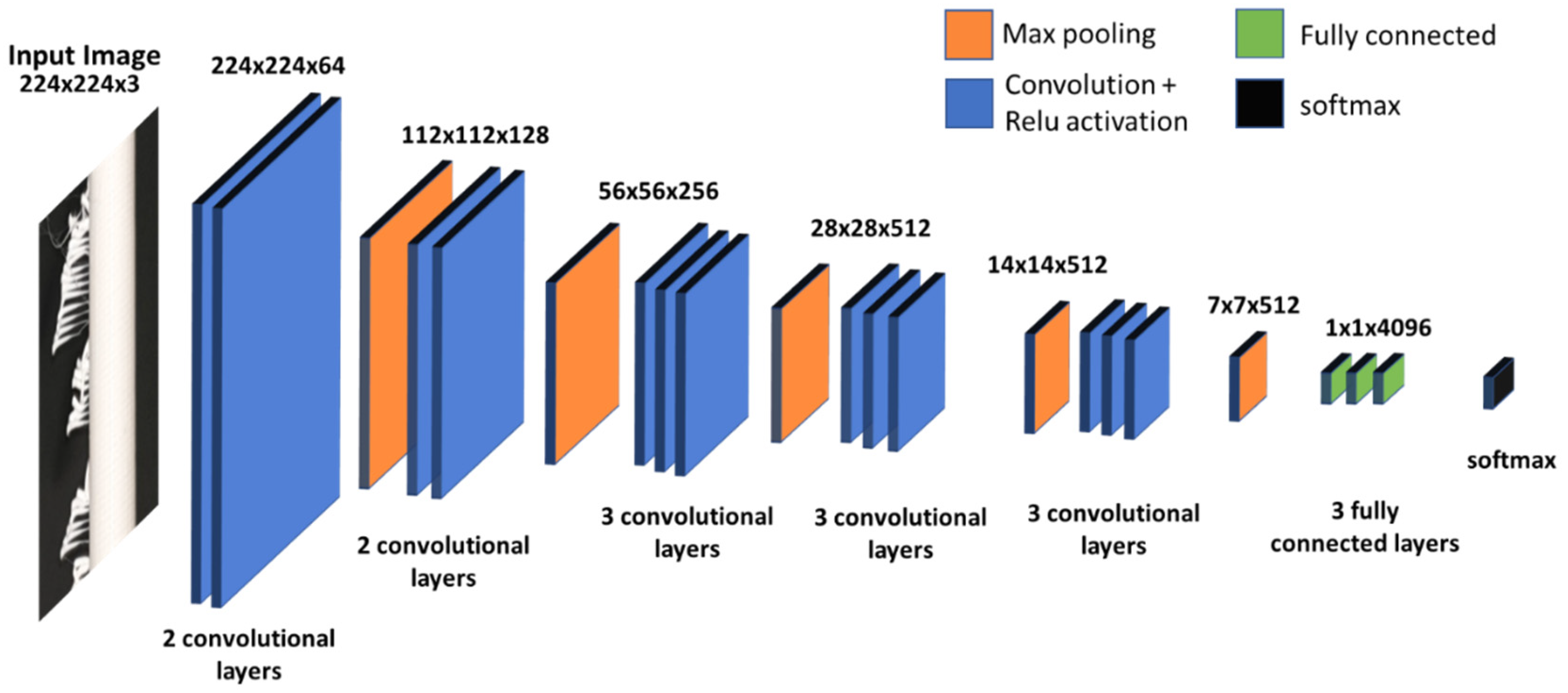
2.2. Model Selection and Training

A wide range of existing state of the art algorithms is available, varying in terms of training speed, accuracy and testing speed in benchmark datasets. In our case, we considered the need to balance between good accuracies and fast detection, as the purpose of the model usage is to be deployed in a live environment. In this sturdy, the selected model was the Single Shot Detector.
The Single Shot Detector running on 300 × 300 input (SSD-300), published in 2016, achieved a mean Average Precision (mAP) of 74.3% on benchmark Dataset VOC-2007 at 59 frames per second (FPS) and a mean Average Precision (mAP) of 41.2% at an Intersection over Union (IoU) of 0.5 on benchmark Dataset of Common Objects in Context (COCO test-dev2015) [25]. The achieved mAP outperformed existing (at the time) state-of-the-art models while running at high FPS. Other advantages of SSD models are the runtime speed at live applications as well as the reduced training time. There is also a Single Shot Detector running on 512 × 512 input frames (SSD-512) with higher achieved mAP on VOC-2007 (76.8%). We selected the SSD-300 due to its superiority in FPS compared to SSD-512 (59 vs. 22) and due to its light requirements in input resolution, as the there was a need to run the model also in low-quality cameras.
The Single Shot Detector consists of two phases: In the first, there is a feed-forward convolutional network (used as typical image classifier) that has a fixed size collection of bounding boxes as output. The used convolutional network is VGG16 [26], which is based on standard convolutional neural network (CNN) architectures: Multiple convolution layers and ReLU activations followed by max pooling functions are producing the input to fully connected layer (Figure 2). A final softmax function produces probabilities of the image to belong to a class. In total, there are 16 convolutional layers and 3 fully connected. VGG16 achieved 92.7% test accuracy in ImageNet, which is a dataset of over 14 million images belonging to 1000 classes. It was chosen in our case as the CNN network, due to its reliability in image classification tasks as well as due to its use in the original SSD-300 publication [25]. In the SSD architecture, the described VGG16 is called the base network.
In this stage, a score is given to each box referring to the probability of presence of an object class. Then, extra convolutional layers are added at the end of the base network, whose size decreases progressively until reaching a non-maximum suppression [25]. These extra layers can help detect at multiple scales. The non-maximum suppression decides the final detections with use of the extra convolutional feature layers at the end first network. The selected model was trained with use of the Tensorflow application programming interface (API) [27] and on a NVIDIA Tesla K80 GPU with 2496 cores of Compute Unified Device Architecture (CUDA) and 12GB of Graphics Double Data Rate (GDDR5) Video Random Access Memory (VRAM). Our selected hyperparameters for the trained model architecture of Figure 3 are presented in Table 2. The methodology for the development of the Deep Neural Network for detecting stringing defects is presented in Figure 4.

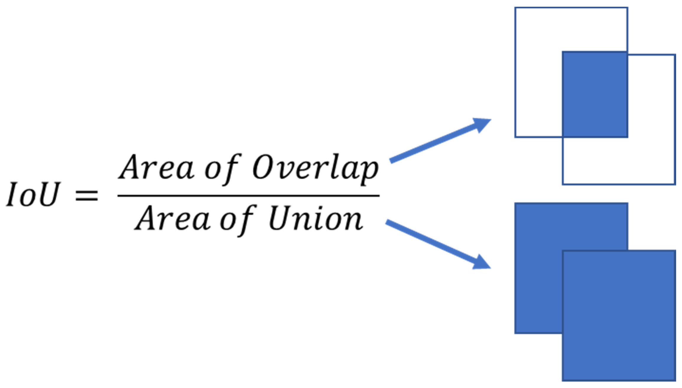
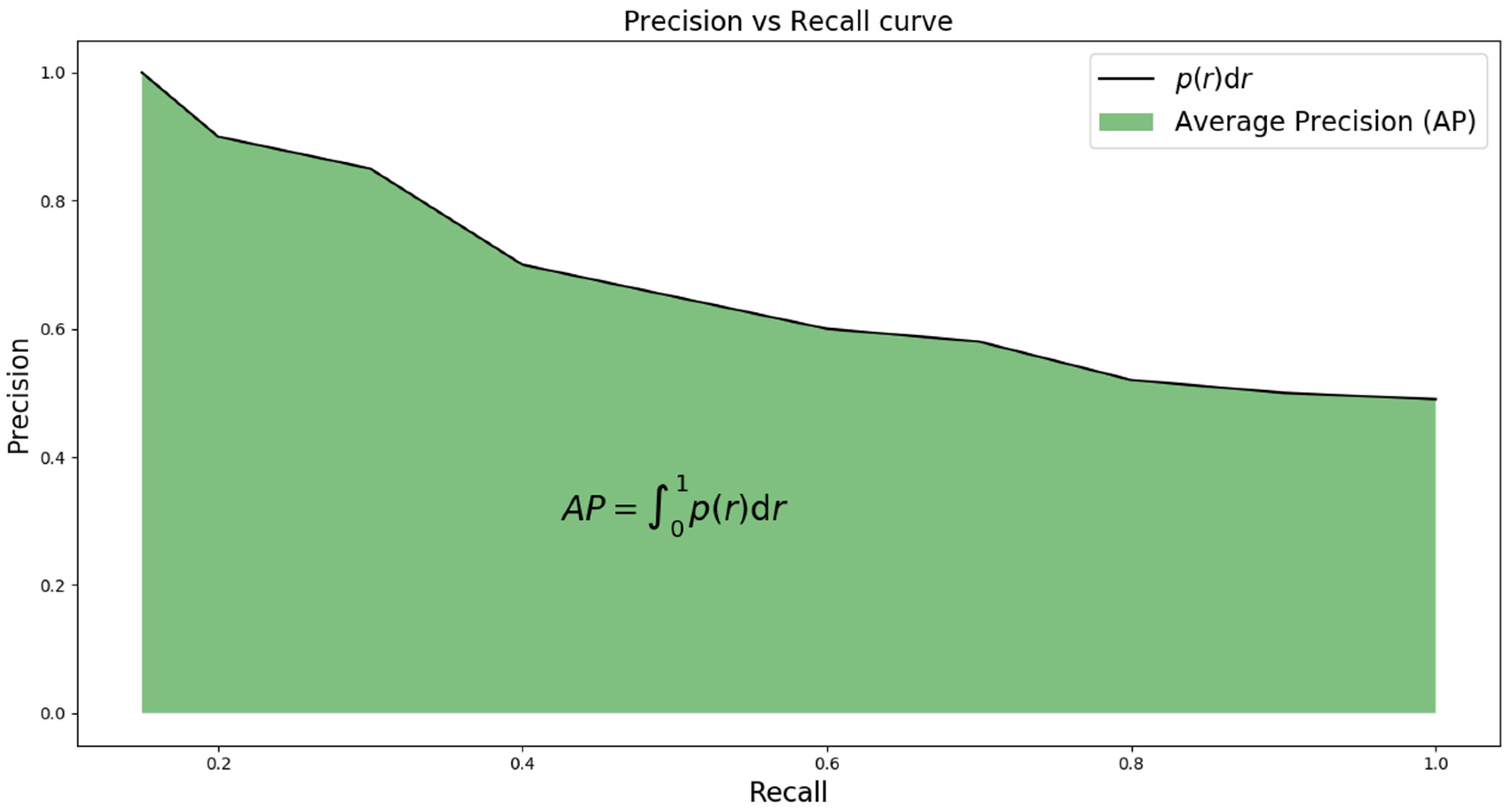
2.3. Evaluation Metrics Principles

In order to evaluate the detection results of the developed neural network, a proper metric is defined. As object detection algorithms use bounding boxes to make local prediction, the Intersection over Union (IoU) helps to quantify the precision of a specific predicted bounding box (Figure 5). IoU measures the overlap between two bounding boxes. Specifically, IoU quantifies the amount of overlap of the predicted bounding box and the ground truth bounding box. In our case, we experimented with a threshold of 0.4, 0.5 and 0.6 as the margin for true or false predictions. In the case of an IoU equal to 0.5, if the IoU value of a specific bounding box is greater than 0.5, we consider this a true positive prediction. This can be further used to calculate the True Positives, False Positives or False Negatives of the models given a test set. In our case, we do not evaluate True Negatives, as each image in the test set has at least one defect.
When the IoU is greater than 0.5 (threshold), the respective prediction is a True Positive (TP), meaning that the predicted defect was real. In cases where the IoU is less than 0.5, we have a False Positive (FP), meaning that the predicted defect was not real. Finally, when the model completely misses a true defect, we consider this a False Negative (FN). The above cases are presented in Figure 6, Figure 7, Figure 8 and Figure 9.
After computing the above rates, the Precision, Recall and F1-Score are calculated.
P r e c i s i o n = T P T P + F P R e c a l l = T P T P + F N F 1 = 2 * P r e c i s i o n * R e c a l l P r e c i s i o n + R e c a l l
Each prediction (whether it is TP or FP) comes with a probability score (probability that a bounding box contains a defect). Ordering all of the predictions with descending order according to the confidence level (0 to 1.0), one can compute how Precision and Recall are changing with respect to the confidence level by plotting their values in a Precision vs. Recall plot (Figure 10). Our final metrics will be the Precision and Recall. In addition, the Average Precision, which is defined as the area under the Precision–Recall curve can also help identify the pros and cons of selecting each probability threshold with respect to the discrimination ability of the classifier. Average Precision can be interpreted mathematically as the weighted mean of precisions achieved at each probability score, with the increase in recall from the previous threshold used as the weight. Average Precision is used as a metric in the development of state-of-the-art models as well as in benchmark dataset challenges [28].

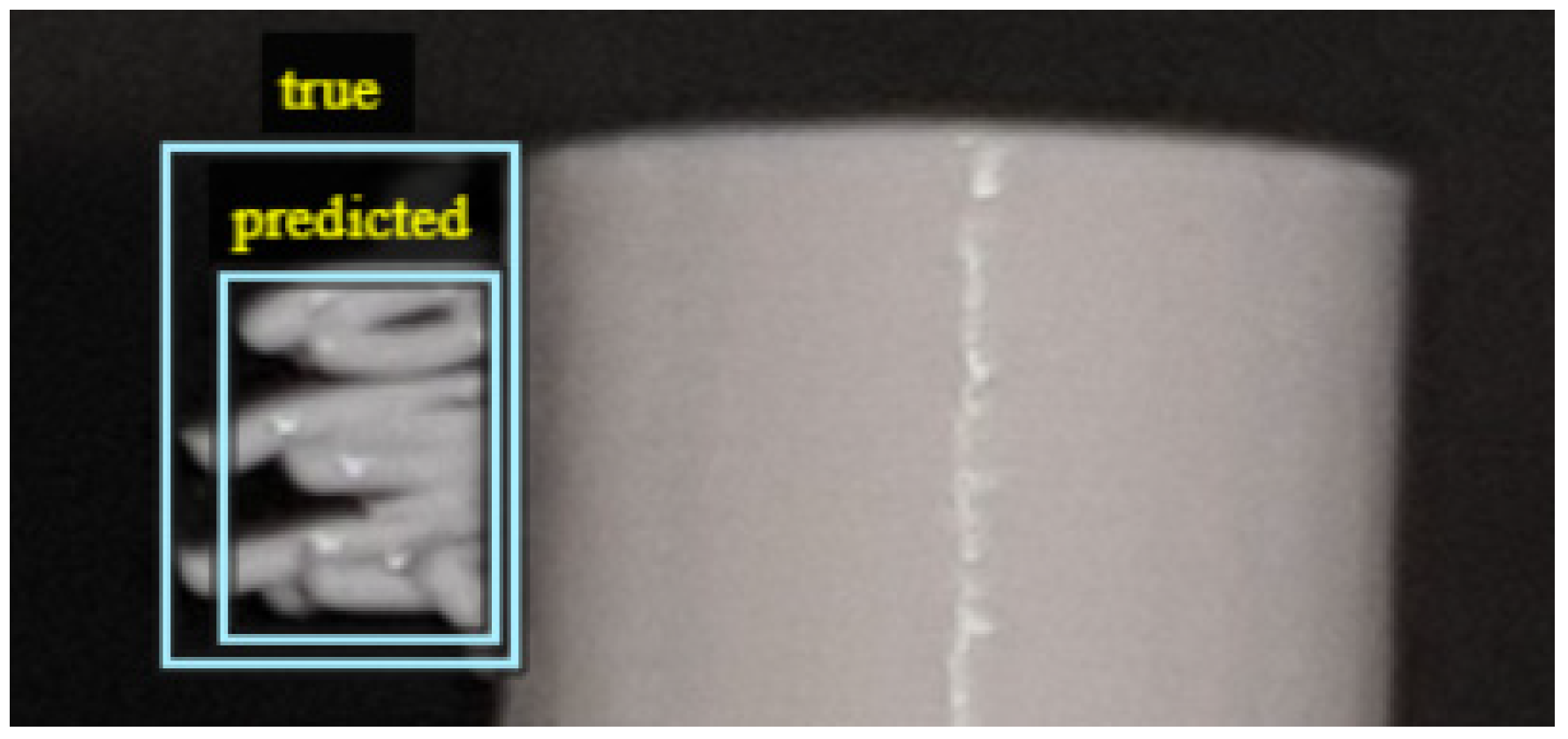
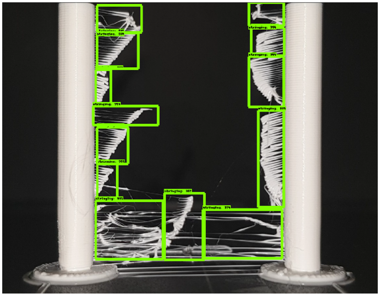
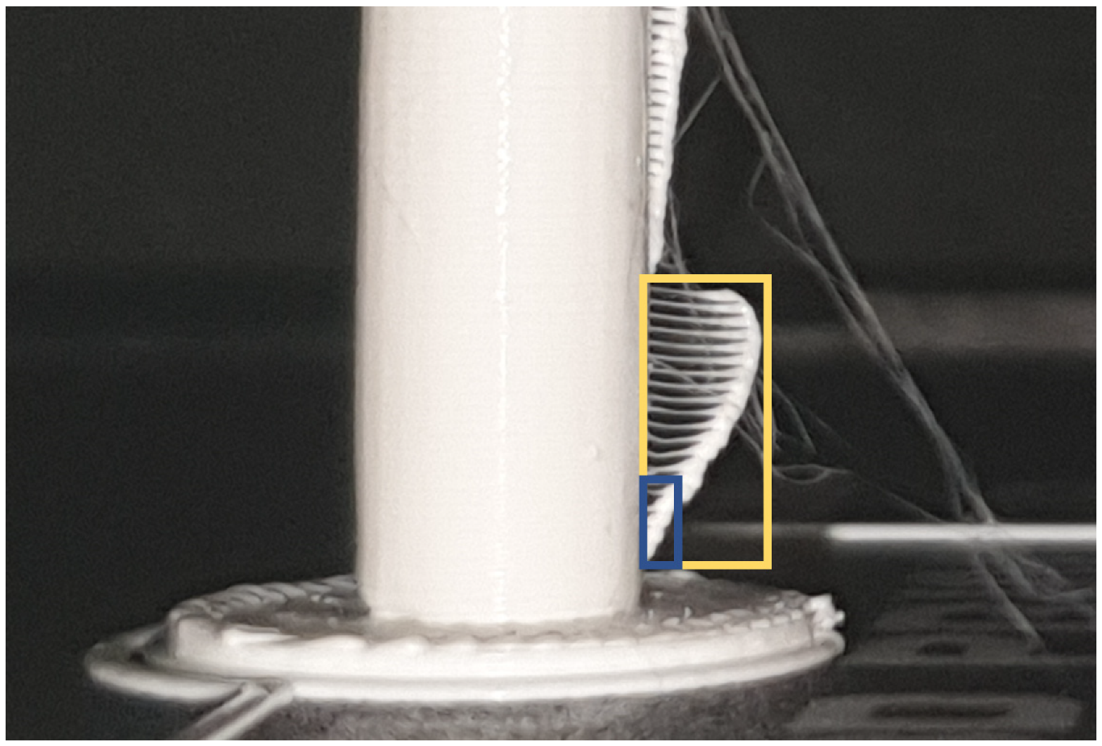
3. Results and Live Deployment

The trained model achieved a Precision of 0.44 and a Recall of 0.69 at an IoU of 0.4, a Precision of 0.41 and a Recall of 0.63 at an IoU of 0.5, and a Precision of 0.4 and a Recall of 0.62 at an IoU of 0.6. Increasing the IoU threshold, predictions are forced to be more strict, resulting in less accurate metrics. We found that the threshold of 0.4 IoU is often selected in similar custom object detection tasks [29,30,31,32], whereas the most used value is 0.5. However, it might result in having more False Positives (lower precision), as the threshold of approving the classifier’s guess becomes higher. An IoU threshold of 0.4 is acceptable in our case, as we need just a little intersection over union between ground truth and prediction: a predicted defect overlapping at least 40% with any given true defect should be considered as a true positive and be handled as a defect (Figure 11). With the current training data, if we wish to increase the number of true defects that are detected (True Positives), we need to keep the IoU threshold to this minimum. Below 0.4, values of IoU threshold result in significant high false detection (False Positives). Therefore, increasing the IoU threshold will give less True Positives but also less False Positives. Choosing a value for the IoU threshold is an issue of balancing between these two. In our case, we selected to be alarmed (defect detection) even falsely rather than not being alarmed at all. A high Precision is needed when the cost of False Positives (normalities detected as defects) is high. On the other, a high Recall is preferred when the cost of False Negatives (real defects not being detected at all) is high. In our case, the cost of missing defects is higher compared to the cost of predicting stringing defects to a normal print. Specifically, we prefer to be alarmed falsely (False Positive–Low precision) than miss defects (False Negative–Low recall). Therefore, we chose the trained model with an IoU threshold of 0.4 (Precision of 0.44 and a Recall of 0.69) for live deployment.
The F1-Score for the IoU threshold of 0.4 is 0.55. There are some aspects around this number that are promising signs for future improvements: the original 500 images are considered not enough, as we need to predict shapes (stringing) of various geometries. Accuracy metrics are therefore expected to increase if we significantly increase the training data. Creation of new data should be also focused on rarely seen (in current training) cases. Regarding Average Precision, the trained SSD model reached 0.4 at an IoU threshold of 0.6, 0.44 at an IoU threshold of 0.5 and 0.52 at an IoU threshold of 0.4. Research on benchmark datasets [28,32] has shown that Average Precision is a good metric for identifying bad or insufficient training data for a specific class. This approach can be useful and efficient, when the goal is to detect known stringing defects. In other words, the expected input images in a real environment will be similar to the training data. Our trained model was able to achieve a Precision of 0.75 and a Recall of 0.92 when seeing the training data (training F1-Score 0.82). This result shows that the use of recently developed Neural Networks can help automate detections of defects with expected shape or low variety. The trained model was considered to perform well in this work and therefore can be used as an automated way of detecting stringing and sending respective notifications. This study is serving as a proof of concept that Deep Learning can be used for the detection of standard and expected stringing defects and specifically when the input video feed in the deployed model is expected to be similar to the training data that the model has seen. Such a prediction on a video frame is illustrated in Figure 12.
However, our model did not perform well when applied on external data acquired from the web (with and without defects). The observed lack of generalization was expected, as the training data included case-specific images. Specifically, only a few shapes and on a specific 3D printer environment were addressed. In order to generalize better, the model needs continuous improvement through training on new and previously not seen data.
Another aspect of the metrics that need to be addressed is the ability of the detector model to identify defects on different time steps of the defect creation. For instance, the model was able to detect stringing defects even on early stages, while the defect was small. This can be attributed to the appropriate annotation on training data. Specifically, our training data annotation was created in such a way that both early and late stages of defect’s appearance were included (Figure 13); this helped the trained model to “learn” both cases.
Regarding computational requirements and performance, the results are promising as the model can very quickly make a detection on a given live video feed. The setup was able to run at 14 frames per second (FPS) video, giving real-time output.
Our next step was to deploy this model on a live 3D printing environment. This was achieved by running the model on a Raspberry Pi 4 microprocessor (with a connected camera), which was placed properly in front of the printing bed. The model was running at the same FPS rate on the microprocessor. A second simpler algorithm was running on top of the model, while analyzing its predictions and its probability scores. Specifically, at each frame, the wrapper algorithm was used a decision support system for the process control. If the probability score of any given predicted defect was greater than a predefined value, the algorithm notified the user on whether or not to stop the 3D printing process. This setup was used as a remote monitoring system for long prints of shapes that are similar to the training Data. Our future work includes continuous training of the model on new cases (object shapes, stringing shapes and scales, printer environments) in order to meet a more holistic approach.

4. Conclusions

A deep neural network (Single Shot detector) was trained on—manually annotated—images of 3D printed objects with a developed stringing defect and deployed on a live environment in order to test its ability to quickly and accurately predict this defect. The model was able to identify defects and also with proper adjustments to the algorithm to notify the printer handler on events with a high probability of defect. The model achieved a Precision of 0.44 and a Recall of 0.69 in the test set; however, it was not able to generalize well in external Datasets. This study highlights the potential and effectiveness of using Deep Learning for detecting 3D printing defects with expected structure and shape, as our model successfully detected defects that are similar to the training Data (training accuracy). Major benefits of such an approach are the fast and real-time detections (59 FPS) and the absence of camera or equipment calibration. This tool can be used as a remote monitoring system of 3D printing processes. It can also help minimize printing costs (raw materials, etc.), as the operator is notified on time about possible defects and can terminate the process on early stages. We propose that defect-specific detection modules can be developed and refined in a distinct mode, as presented in this work. The integration of different defect-detection components can support the development of more generalized tools, alleviating several of the issues that detecting a multitude of very distinctive process errors through a single approach could introduce. Our future work includes the ability of the AI system to intervene on the printing parameters of the process and correct (or adjust) them properly in order to minimize the defect as the printing process continues.

Author Contributions

Conceptualization, K.P., P.K. and E.P.K.; methodology, K.P., P.K. and E.P.K.; software, K.P., P.K. and E.P.K.; validation, K.P., P.K. and E.P.K.; formal analysis, K.P., P.K. and E.P.K.; investigation, K.P., P.K. and E.P.K.; resources, K.P., P.K. and E.P.K.; data curation, K.P., P.K. and E.P.K.; writing—original draft preparation, K.P., P.K. and E.P.K.; writing—review and editing, K.P., P.K. and E.P.K.; visualization, K.P., P.K. and E.P.K.; supervision, K.P., P.K. and E.P.K.; project administration, K.P., P.K. and E.P.K.; funding acquisition, K.P., P.K. and E.P.K. All authors have read and agreed to the published version of the manuscript.

Funding

This research received no external funding.

Conflicts of Interest

The authors declare no conflict of interest.

References

  1. Szeliski, R. Computer Vision: Algorithms and Applications; Springer Science & Business Media: Amsterdam, The Netherlands, 2010. [Google Scholar]
  2. El-Dahshan, E.-S.A.; Hosny, T.; Salem, A.-B.M. Hybrid intelligent techniques for MRI brain images classification. Digit. Signal Process. 2010, 20, 433–441. [Google Scholar] [CrossRef]
  3. Starner, T.; Auxier, J.; Ashbrook, D.; Gandy, M. The gesture pendant: A self-illuminating, wearable, infrared computer vision system for home automation control and medical monitoring. In Proceedings of the Digest of Papers. Fourth International Symposium on Wearable Computers, IEEE, Atlanta, GA, USA, 21 October 2000. [Google Scholar]
  4. Agin, G. Computer Vision Systems for Industrial Inspection and Assembly. Computer 1980, 13, 11–20. [Google Scholar] [CrossRef]
  5. Kurada, S.; Bradley, C. A review of machine vision sensors for tool condition monitoring. Comput. Ind. 1997, 34, 55–72. [Google Scholar] [CrossRef]
  6. Menze, M.; Geiger, A. Object scene flow for autonomous vehicles. In Proceedings of the 2015 IEEE Conference on Computer Vision and Pattern Recognition (CVPR), Boston, MA, USA, 12 June 2015; pp. 3061–3070. [Google Scholar]
  7. Hou, Y.-L.; Pang, G.K.H. People Counting and Human Detection in a Challenging Situation. IEEE Trans. Syst. Man Cybern. 2014 Part A Syst. Humans 2010, 41, 24–33. [Google Scholar] [CrossRef] [Green Version]
  8. Scime, L.; Beuth, J. Anomaly detection and classification in a laser powder bed additive manufacturing process using a trained computer vision algorithm. Addit. Manuf. 2018, 19, 114–126. [Google Scholar] [CrossRef]
  9. Baumgartl, H.; Tomas, J.; Buettner, R.; Merkel, M. A deep learning-based model for defect detection in laser-powder bed fusion using in-situ thermographic monitoring. Prog. Addit. Manuf. 2020, 5, 1–9. [Google Scholar] [CrossRef] [Green Version]
  10. Cui, W.; Zhang, Y.; Zhang, X.; Li, L.; Liou, F. Metal Additive Manufacturing Parts Inspection Using Convolutional Neural Network. Appl. Sci. 2020, 10, 545. [Google Scholar] [CrossRef] [Green Version]
  11. Jin, Z.; Zhang, Z.; Gu, G.X. Automated Real-Time Detection and Prediction of Interlayer Imperfections in Additive Manufacturing Processes Using Artificial Intelligence. Adv. Intell. Syst. 2020, 2, 1900130. [Google Scholar] [CrossRef] [Green Version]
  12. Nuchitprasitchai, S.; Roggemann, M.; Pearce, J.M. Factors effecting real-time optical monitoring of fused filament 3D printing. Prog. Addit. Manuf. 2017, 2, 133–149. [Google Scholar] [CrossRef] [Green Version]
  13. Petsiuk, A.; Pearce, J.M. Open source computer vision-based layer-wise 3D printing analysis. arXiv 2003, arXiv:05660. [Google Scholar] [CrossRef]
  14. All3dp. Available online: https://all3dp.com/2/ender-3-filament-sensor-runout/ (accessed on 13 October 2020).
  15. Re3dp. Available online: https://re3d.org/gigabot/ (accessed on 13 October 2020).
  16. Langeland, S.A.K. Automatic Error Detection in 3D Pritning using Computer Vision. Master’s Thesis, The University of Bergen, Bergen, Norway, 2020. [Google Scholar]
  17. OpenCV. Available online: https://opencv.org/ (accessed on 13 October 2020).
  18. Baumann, F.; Roller, D. Vision based error detection for 3D printing processes. MATEC Web Conf. 2016, 59, 06003. [Google Scholar] [CrossRef]
  19. Lyngby, R.A.; Wilm, J.; Eiríksson, E.R.; Nielsen, J.B.; Jensen, J.N.; Aanæs, H.; Pedersen, D.B. In-Line 3D Print Failure Detection Using Computer Vision; euspen: Leuven, Belgium, 2017. [Google Scholar]
  20. Makagonov, N.G.; Blinova, E.M.; Bezukladnikov, I.I. Development of Visual Inspection Systems for 3D Printing. In Proceedings of the 2017 IEEE Conference of Russian Young Researchers in Electrical and Electronic Engineering (EIConRus), Moscow, Russia, 1–3 February 2017. [Google Scholar]
  21. Karayannis, P.; Petrakli, F.; Gkika, A.; Koumoulos, E. 3D-Printed Lab-on-a-Chip Diagnostic Systems-Developing a Safe-by-Design Manufacturing Approach. Micromachines 2019, 10, 825. [Google Scholar] [CrossRef] [PubMed] [Green Version]
  22. OctoPrint. Available online: https://octoprint.org/ (accessed on 13 October 2020).
  23. Perez, L.; Wang, J. The effectiveness of data augmentation in image classification using deep learning. arXiv 2017, arXiv:1712.04621. [Google Scholar]
  24. Tzutalin, L. Git Code. 2015. Available online: https://github.com/tzutalin/labelImg (accessed on 13 October 2020).
  25. Liu, W.; Anguelov, D.; Erhan, D.; Szegedy, C.; Reed, S.; Fu, C.Y.; Berg, A.C. Ssd: Single Shot Multibox Detector. In Proceedings of the European Conference on Computer Vision, Amsterdam, The Netherlands, 8–16 October 2016. [Google Scholar]
  26. Simonyan, K.; Zisserman, A. Very deep convolutional networks for large-scale image recognition. arXiv 2014, arXiv:1409.1556. [Google Scholar]
  27. TensorFlow. Available online: https://www.tensorflow.org/ (accessed on 13 October 2020).
  28. Everingham, M.; Van Gool, L.; Williams, C.K.I.; Winn, J.; Zisserman, A. The Pascal Visual Object Classes (VOC) Challenge. Int. J. Comput. Vis. 2010, 88, 303–338. [Google Scholar] [CrossRef] [Green Version]
  29. Zhang, H.; Kyaw, Z.; Chang, S.F.; Chua, T.S. Visual Translation Embedding Network for Visual Relation Detection. In Proceedings of the IEEE Conference on Computer Vision and Pattern Recognition, Honolulu, HI, USA, 21–26 July 2017; pp. 5532–5540. [Google Scholar]
  30. He, X.; Peng, Y.; Zhao, J. Fine-Grained Discriminative Localization Via Saliency-Guided Faster R-CNN. In Proceedings of the 25th ACM International Conference on Multimedia, New York, NY, USA, 23–27 October 2017; pp. 627–635. [Google Scholar]
  31. Halstead, M.; McCool, C.; Denman, S.; Perez, T.; Fookes, C. Fruit quantity and quality estimation using a robotic vision system. arXiv 2018, arXiv:1801.05560. [Google Scholar]
  32. Tian, Z.; Shen, C.; Chen, H.; He, T. Fcos: Fully Convolutional One-Stage Object Detection. In Proceedings of the IEEE International Conference on Computer Vision, Seoul, Korea, 27 October–2 November; pp. 9627–9636.
Figure 1. Stringing defect in 3D printed object.
Processes 08 01464 g001
Figure 2. Architecture of the VGG16 used in the Single Shot Detector (SSD).
Processes 08 01464 g002
Figure 3. The Single Shot Detector on 300 × 300 input images.
Processes 08 01464 g003
Figure 4. Methodology for the development of the Neural Network for stringing detection.
Processes 08 01464 g004
Figure 5. Intersection over Union schematic representation.
Processes 08 01464 g005
Figure 6. Intersection over Union (IoU) > 0.5 (TP) for printed sample.
Processes 08 01464 g006
Figure 7. No detection at all (FN) for printed sample.
Processes 08 01464 g007
Figure 8. IoU < 0.5 (FP) for printed sample.
Processes 08 01464 g008
Figure 9. IoU < 0.5 (FP) for printed sample.
Processes 08 01464 g009
Figure 10. Precision vs. Recall curve and the Average Precision metric.
Processes 08 01464 g010
Figure 11. IoU of 0.4, schematically presented at inset.
Processes 08 01464 g011
Figure 12. Predictions on a test image.
Processes 08 01464 g012
Figure 13. Annotation approach for both early and late stages of stringing appearance.
Processes 08 01464 g013
Table 1. Summary table of pros and cons of existing applications.
Approach CategoryProsCons
Comparison of final printed object with reconstruction of 3D printed model [12]
  • High rates of defect detection
  • Low cost
  • generalization in different object geometries, filament colors
  • Ability to integrate decision making
  • Clogged nozzle and loss of filament detections
  • Defects (clogged nozzle, loss of filament, incompleteness) of subject can be rare for experienced users
  • Slow computation time
  • In need for calibration and configuration of printer for different cases
  • May require more than one camera
  • Small-scale defects not identified
  • Use case specific
Combination of conventional Image processing techniques (layer-wise) [13,16]
  • Various types of defects can be detected
  • Decision making based on defect identification
  • High rates of detection on use cases
  • Can also detect small-scale failures
  • Not tested in multiple geometries
  • Not generalizable
  • May need calibration and configuration of printer for different cases
  • Slow
  • The discriminative power of the failure detection depends on the resolution of the camera, the distance to the print area, the size of the par
  • fault detection relies on a single threshold, which is usually case specific
  • Image thresholding requires parameter determination on each image case
  • May require more than one camera
Advanced Image Processing [18,19]
  • Early failure detection
  • Image processing parameters can be determined by asking users’ input on the UI
  • Fast and real time
  • Detachment from print bed, not continuous material flow from nozzle and printed object deformation
  • Simple setup
  • Exact camera position calibration
  • Image thresholding requires parameter determination on each image case
  • Smoothing out the image feed consumes additional computational resources.
  • Only a few defects
  • Available only for low video resolution
Table 2. Hyperparameters of the SSD-300 trained.
Batch_Size24
initial_learning_rate0.004
decay_steps800
decay_factor0.95
momentum_optimizer_value0.9
decay0.9
epsilon1.0
Publisher’s Note: MDPI stays neutral with regard to jurisdictional claims in published maps and institutional affiliations.

