Article

Energy–Water Management System Based on Predictive Control Applied to the Water–Food–Energy Nexus in Rural Communities

1
Department of Electrical Engineering, Universidad de Chile and Instituto Sistemas Complejos de Ingeniería (ISCI), Santiago 8370451, Chile
2
Department of Electrical Engineering, Universidad de La Frontera, Temuco 4811230, Chile
3
Department of Geology and Centro de Excelencia en Geotermia de los Andes (CEGA), Universidad de Chile, Santiago 8370451, Chile
*
Author to whom correspondence should be addressed.
These authors contributed equally to this work.
Appl. Sci. 2020, 10(21), 7723; https://doi.org/10.3390/app10217723
Submission received: 2 September 2020 / Revised: 17 October 2020 / Accepted: 21 October 2020 / Published: 31 October 2020
(This article belongs to the Special Issue Water-Energy-Environment Nexus (WEEN-2019))

Abstract

:
Generating strategies and techniques to feed the increasing world population is a significant challenge under climate change effects such as drought. Rural areas are especially sensitive to such effects as they are unable to overcome the lack of water with new agricultural production techniques. In developing countries, rural communities commonly do not have access to high-quality electricity supplies. In some cases, these communities lack electricity in their homes, which affects the opportunity to improve food production through the incorporation of new technologies. This work proposes an integrated optimizer based on model predictive control (MPC) that combines a water management system, which handles the medium-term water requirements for irrigation, with an energy management system, which handles short-term energy requirements. The proposed approach is based on predictive phenomenological models of evapotranspiration and electricity consumption considering climate conditions such as temperature, precipitation, solar radiation, and wind speed, and aims to optimize the use of energy and water and the relative yields of crops. The integrated energy–water management system (EWMS) improves water resource sustainability according to energy availability/costs and water use requirements. Simulation results using real data from a rural community in southern Chile show that the integrated EWMS based on an MPC optimizer successfully determines and satisfies the water and energy requirements under aquifer sustainability constraints.

Graphical Abstract

1. Introduction

With an estimated 30% increase in population by 2050 [1], the challenge of feeding the additional 2.3 billion people in the world is significant. A study by the International Renewable Energy Agency [2] concluded that an increase of 50% in demand for food and water is expected, along with a doubling in the demand for energy, by 2050. This issue has motivated recent studies on the water–food–energy nexus in an attempt to understand the relationship between these three concepts [3,4]. Microgrids have been promoted as a potential technology for electricity provision to worldwide rural communities [5,6], and several studies have addressed their relevance for human well-being and the future security of such communities [6,7]. Climate change and its short- and medium-term scenarios primarily affect rural communities, where food and water security are not optimal and are often fossil fuel-dependent [6]. The scientific literature suggests that promoting microgrid systems will improve water resilience and food production in rural communities worldwide [6,8,9,10].
There have been few studies on the energy–water nexus at the micro-level (e.g., rural zones) regarding the dynamic relationships between energy and water under uncertain scenarios (such as climate change, which produces water shortages [11]). These scenarios, along with population growth, strongly influence the energy–water nexus, especially for less-populated regions. Analysis of the relationship between energy and water should include all aspects of sustainability, such as technical, social, environmental, and economic factors [12]. Water scarcity requires water treatments that are more energy-intensive, such as desalination, to provide irrigation and drinking water. Thus, the conditions where it is possible to implement energy–water systems should be evaluated under different climate scenarios and population demands, in addition to considering the energy costs (or availability) and water reserves at specific settlements. Zhang et al. [3] proposed a distributed variable-frequency pump system with water storage that was adapted to a district cooling system with large end-use load fluctuations. The authors showed energy consumption reductions of 57% on the hottest days based on weather predictions and the optimization of the energy and water supply. This indicates that the relationship between energy and water should be incorporated into technological solutions for efficient and sustainable management of these resources and the strength of the food nexus.
Agriculture is estimated to be the activity that consumes most of the water from aquifers, reaching 60% of the total water extracted in some cases [13]. This indicates the importance of managing the integration of an energy–water system for agricultural purposes. Karan et al. [11] sized an autonomous photovoltaic system to provide energy to a greenhouse, demonstrating that crop yields have better outcomes relative to unmanaged systems. In contrast, Mérida et al. [14] studied a photovoltaic system coupled to a water pump (without considering storage) to irrigate crops based on defined requirements. Although they swiftly met these requirements, the final crop yields were not evaluated or considered to be limiting the availability of irrigation water. The incorporation of water storage allows better use of energy; hence, Powell et al. [15] showed that applying storage for cotton crops provides an economically profitable system.
Optimization models for water reservoir systems must consider efficiency (maximizing current and future discounted welfare), survivability (ensuring future welfare exceeds minimum subsistence levels), and sustainability (maximizing cumulative improvement over time) [16]. The management of these water reserves may have physical constraints due to equipment, minimum and maximum volumes of extraction and storage, legal obligations, and so on [17]. Brdys et al. [18] used hierarchical predictive control for wastewater management, with a three-layer framework used to consider the different time scales of the involved biological processes. The upper hierarchy layers act in the longer term and send set points to lower levels, which act in the shorter term. The work of Nikam and Regulwar [13] maximized the benefits of crops in a monthly model under constraints associated with cultivated areas to fulfill irrigation quotas and storage boundaries; however, this did not consider the effects of water insufficiency on crop yields. Given the limitations of water availability, the problem is how to distribute water among different crops. For this, the sum of relative crop yields has been maximized without considering aspects such as the crop yield or the expected returns [19]. However, this strategy benefits crops with lower water requirements or small, cultivated areas [20]. Cai et al. [21] weighted the expected yield by the sale price of the crop and determined the distribution of water between different crops. Georgiou and Papamichail [22] and Georgiou et al. [23] also added cultivated areas as a criterion. None of these works considered the minimum yield thresholds that crops must meet as self-consumption criteria.
In Chile and other countries around the world, many rural communities lack adequate access to essential services such as water and electricity, which impacts their quality of life. The access and management of water and energy are conditioned by several territorial aspects and cause many energy–water-linked problems such as water shortages. Additionally, access to electricity generation technology (without any coordination between consumers) could generate indiscriminate water extraction from aquifers at a rate higher than the natural recharge, which would compromise water resource sustainability [24,25]. Chile’s case is explanatory, as the recent droughts in the period 2010–2018 were the longest in recorded history, with a rain deficit of 20–40% [26]. Studies conducted by the Ministry of Environment in Chile [27] indicate that this will become a critical situation in 2050, with a 30% water deficit in the Chilean central valley together with a temperature increase of 3 °C. Thus, Chile can be used as a case study to test the integrated optimization of an energy–water management system as a means of improving development in rural areas and ensuring water resource sustainability.
To adequately manage irrigation without causing aquifer depletion, it is necessary to jointly analyze the energy use and water resource reserves considering integrated management with all sustainable aspects, such as technical, environmental, and economic factors [28]. Thus, the integrated control and management of the energy–water systems is necessary to ensure water resource reserves while considering energy availability/costs under different climate scenarios, such as drought. These aspects are analyzed here using the predictive control framework to consider the future dynamics and coupled behavior of water and energy resources. The main contributions of this work are summarized as follows:
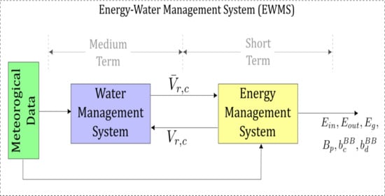
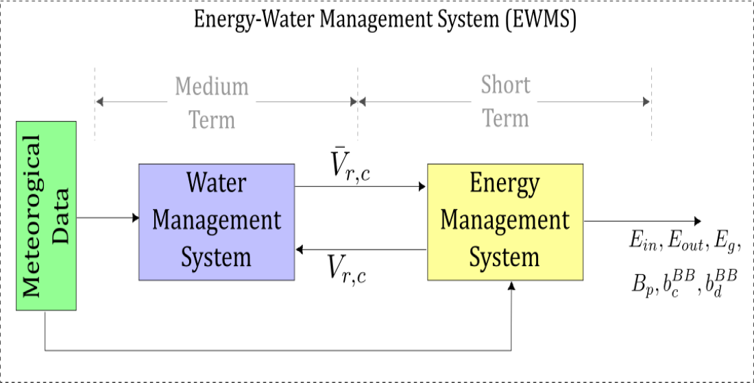
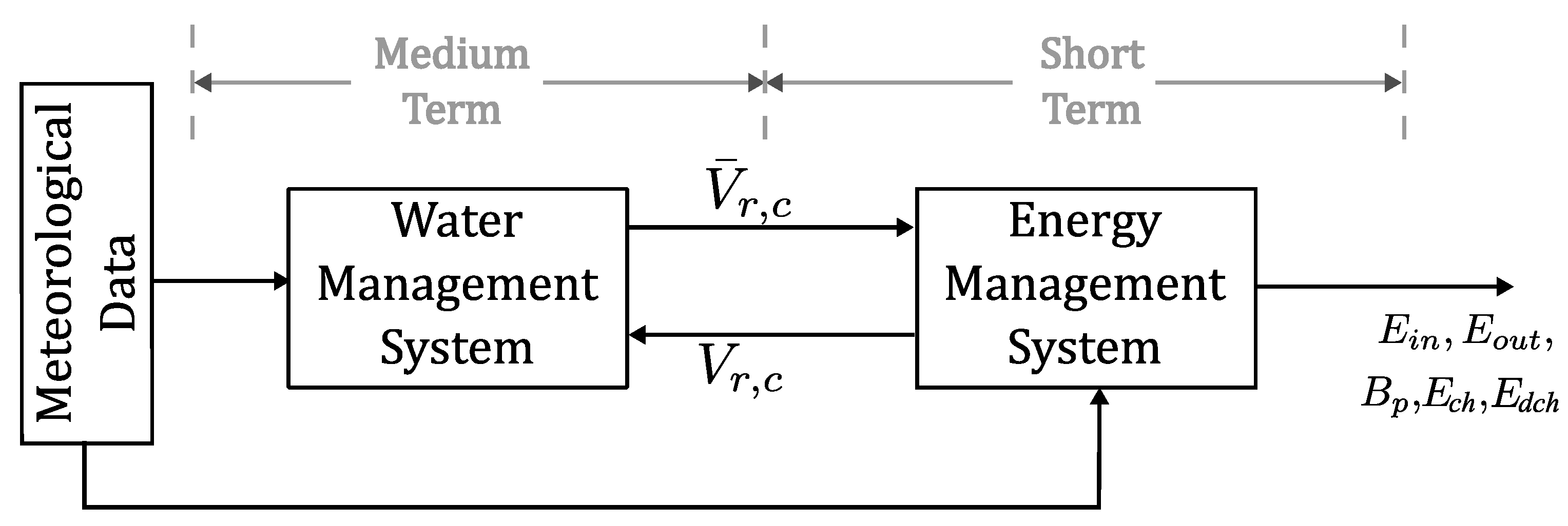
  • A novel energy–water management system (EWMS) is proposed based on the joint optimization of water and energy resources using a model predictive control (MPC) strategy to manage the medium-term water requirements for irrigation and short-term energy requirements for water resource sustainability.
  • A water management system (WMS) based on the MPC technique is proposed to minimize energy costs, including the expected benefits from crops and the availability of energy sources.
  • An electricity management system (EMS) based on the MPC technique is established to include water availability and water use demand.
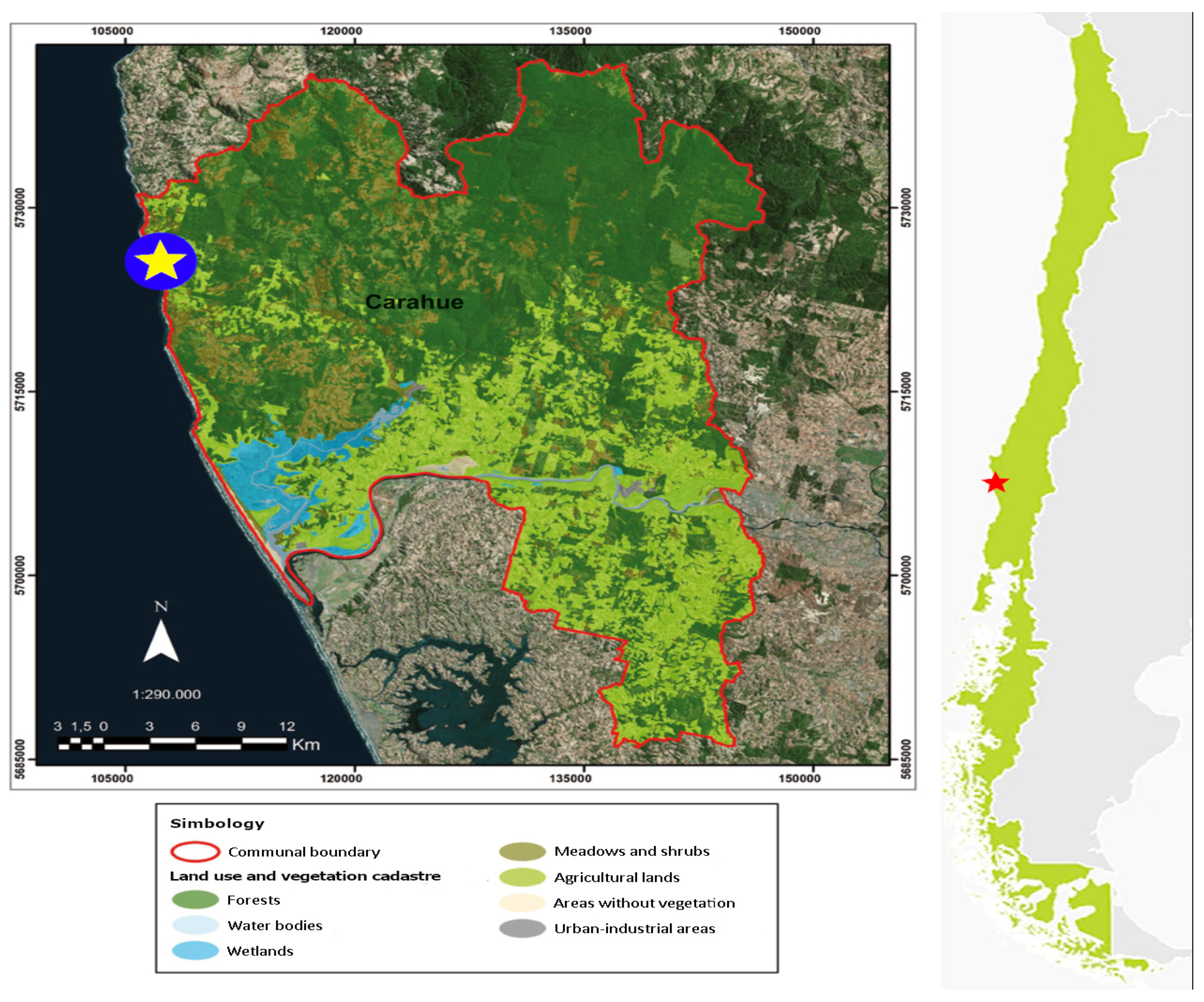
  • The proposed EWMS is validated using real data from a rural community in southern Chile, demonstrating successful performance in terms of determining and meeting water and energy requirements under constraints relative to aquifer sustainability.
The remainder of this paper is organized as follows. In Section 2, the background and models pertaining to aquifers, wells, and irrigation demands are given. In Section 3, the proposed EWMS is described based on predictive control techniques. Section 4 describes the case study used to evaluate the performance of the proposed method, before Section 5 presents simulation results considering real data under three scenarios (normal rain, low rain, and drought). Finally, the conclusions are presented in Section 6.

2. Background

The proposed EWMS based on MPC is designed for and applied to a hydrological system (HS). This corresponds to a well that is fully penetrated into a confined aquifer, a pump, and a tank (see Figure 1). This system has a water volume that is extracted from the well for storage in a tank ( v b ) along with a water requirement for irrigation ( v r ). Each HS can provide water to different crops for the same farmer, each of which has a requirement they must meet, namely v r = i = 1 n v i , r , where n is the number of HS.
Next, the aquifer models, wells, and irrigation demand are described, and the fundamentals of MPC are explained.

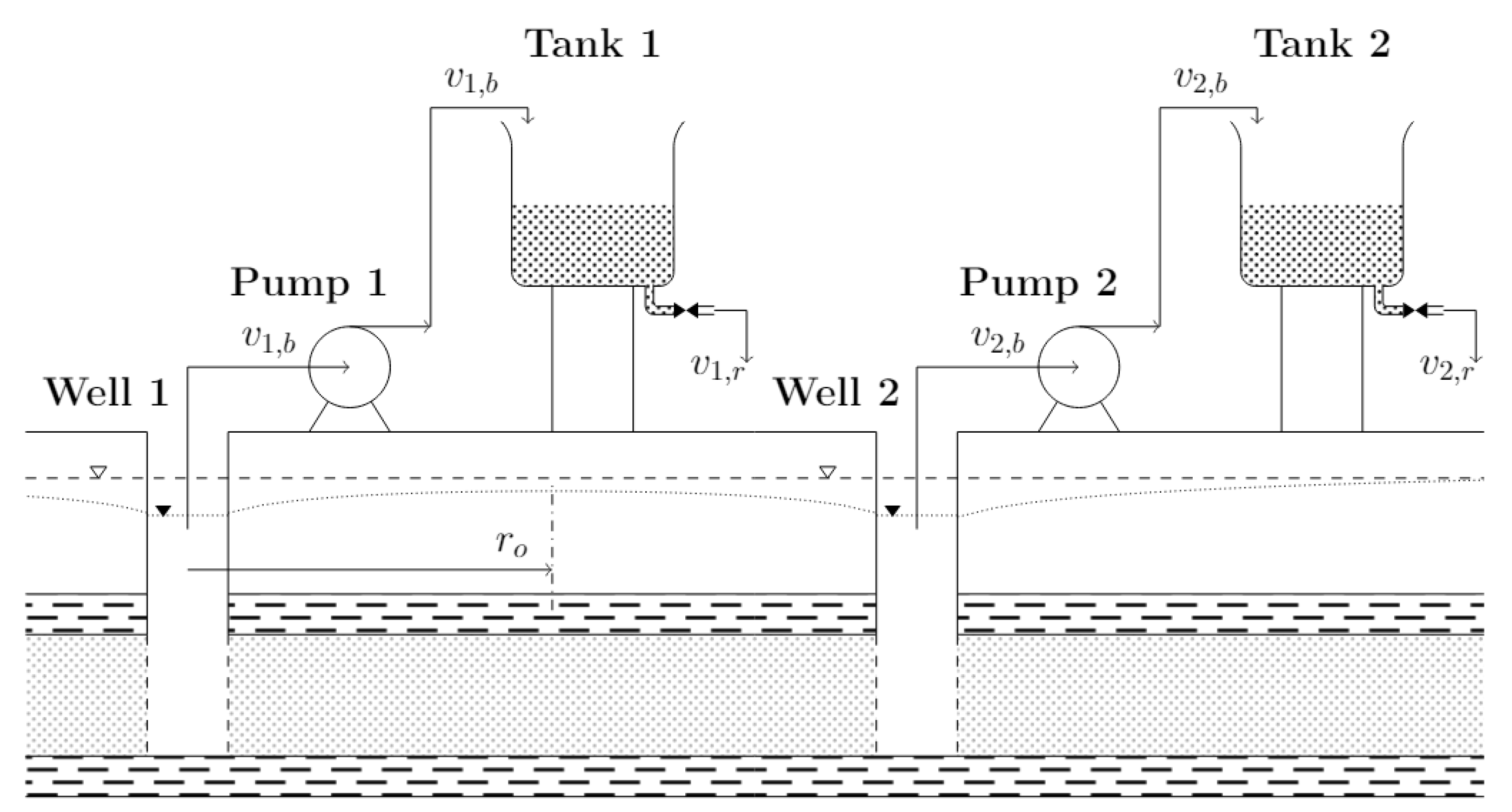
2.1. Aquifer and Well Dynamics

The water table drawdown (s), which is a function of the distance between the pumped wells (r) and the discharging time (t) of a completely penetrative well in a confined aquifer, can be described using the Theis equation [29]:
s ( r , t ) = q 4 π T · W S r 2 4 T t = q 4 π T · W ( u )
where q is the water extraction flow in m/s; T is the transmissivity, defined as the capacity of the aquifer to transmit water, in m 2 /s; and S is the specific storage, defined as the water volume per unit of aquifer volume release when the hydraulic head declines by one unit. W ( u ) represents the well function (or exponential-integral), and is defined as:
W ( u ) = u e x x d x
For intermittent or variable pumping, the principle of superposition in Equation (1) can be used to obtain the following drawdown s at distance r and at time t ( n ) :
s ( r , t ( n ) ) = k = 0 n Δ q ( k ) 4 π T · W S r 2 4 T t ( n ) t ( k )
where Δ q ( k ) = q ( k ) q ( k 1 ) is the increase or decrease in the water flow pumped between two sampling instants, and t ( n ) t ( k ) is the time after pumping q ( k ) began. To ensure zero or minimal interference between wells, the decreasing water level s ( r , t ) must be monitored in terms of its yield. To avoid interactions between wells, the hydraulic threshold ε at a distance r o of less than half the length between two neighboring wells should satisfy s ( r o , t ) ε t .
The hydraulic head drawdown is shown in Figure 1, where the dashed line represents the static hydraulic head and the dotted line indicates the hydraulic head under the pumping conditions calculated by the Theis equation. Following Equation (3), the distance r = r o is the maximum distance with drawdown.
The Chaturvedi formula is used to determine the availability of water that can be extracted from an aquifer. This expression estimates the recharge of an aquifer based on the perceived rainfall in a given area:
R = α ( P β ) γ
where R is the recharge over a year in m, P is the rainfall over a year in m, and the coefficients α , β , and γ depend on the geographic conditions. Typical values are α = 2 , β = 15 , and γ = 0.4 . As this formula is intended to be used over a period of one year, it is modified as follows to obtain the average daily recharge:
R = 2 · 365 T · i = 1 T P ( i ) 15 0.4 · 1 365
where T is the time horizon in days and P ( i ) is the rainfall on day i in inches.

2.2. Irrigation Demand

The daily irrigation demand is determined using a modification of the daily periods used by Raes et al. [30] to the Jensen relative yield equation [31]:
Y r = Y a Y m a x = i = 1 N j = 1 M i 1 K y ( i ) · 1 E T a ( j ) E T p ( j ) 1 / M i
where Y a is the actual yield, Y m a x is the maximum yield, N is the number of growth stages, K y ( i ) is a response factor in the absence of water for each of the stages of the crop, and M i is the duration of each growth stage in days. To obtain Y r = 1 where Y a = Y m a x , the actual evapotranspiration of the crop must be equal to the potential, i.e., E T a ( j ) = E T p ( j ) . Evapotranspiration calculations are obtained from the reference evapotranspiration E T o as measured in mm/day according to the Penman—Monteith equation [32]:
E T o ( k ) = 0.408 Δ ( k ) · ( R n ( k ) G ( k ) ) + γ 900 T ( k ) + 273 u 2 ( k ) · ( e s ( k ) e a ( k ) ) Δ ( k ) · + γ ( 1 + 0.34 u 2 ( k ) )
where G is the thermal flux density in MJ/m 2 day, R n is the net radiation in MJ/m 2 day, T is the average daily temperature in °C, u 2 is the average wind speed at a height of 2 m in m/s, e s is the saturation vapor pressure in kPa, e a is the actual vapor pressure in kPa, Δ is the slope of the vapor saturation pressure with temperature in kPa °C, and γ = c p P 0.622 λ is the psychrometric constant in kPa °C, where c p is the specific heat at a constant pressure in kJ/kg °C, λ is the latent heat of vaporization in MJ/kg, and P is the atmospheric pressure in kPa. From E T o , the potential evapotranspiration ( E T p ) in which there are no irrigation restrictions on the crop is obtained as [33]:
E T p ( k ) = K c ( k ) · E T o ( k ) ,
where K c is a dimensionless coefficient that depends on the crop and its growth stage.
If there are no water limitations for irrigation, the actual evapotranspiration is equal to the potential ( E T a ( k ) = E T p ( k ) ). Otherwise, the lowest available water content in the land implies that E T a ( k ) < E T p ( k ) . The generated stress is quantified with the coefficient K s ( k ) , which relates the supplied irrigation water with the crop yield for day k [34]:
E T a ( k ) = K s ( k ) · E T p ( k ) = K s ( k ) · K c ( k ) · E T o ( k ) ,
K s ( k ) = { T A W ( k ) D r ( k ) T A W ( k ) R A W ( k ) if R A W ( k ) < D r ( k ) , 1         otherwise ,
T A W ( k ) = 1.000 · ( θ F C θ W P ) · Z r ( k ) ,
D r ( k ) = D r ( k 1 ) P ( k ) + R O ( k ) I ( k ) C R ( k ) + D P ( k ) + E T p ( k ) ,
D r ( 0 ) = 1.000 · ( θ F C θ 0 ) · Z r ( 0 ) ,
I ( k ) = 1 , 000 · V ¯ r , c ( k ) A c ,
0 D r ( k ) T A W ( k ) ,
where T A W is the total available water from the soil in mm, D r is the root zone depletion in mm, R A W is the fraction of T A W for crops that can be extracted from the soil without suffering stress (fulfilling R A W = p · T A W ), θ F C is the water content that the soil naturally retains in m 3 · m 3 , θ W P is the permanent wilting point in m 3 · m 3 , Z r is the depth of roots in m, P is the rainfall in mm, R O is the runoff loss in mm, I is the irrigation in mm, C R is the absorption of water by capillarity in mm, and D P is the water lost by filtration. As the water system shown in Figure 1 uses the yield irrigation requirements, the irrigation I is obtained from the required irrigation volume V ¯ r , c per crop in m 3 and its acreage A c in m 2 .

2.3. Principles of Model Predictive Control

MPC is based on the optimization of future system behavior with respect to future control actions [35]. For MPC design, a discrete nonlinear (or linear) model of the system is required to predict the future behavior; the future control actions u ( k ) , u ( k + 1 ) , . . . , u ( k + N u 1 ) are then calculated by optimizing an objective function with constraints on the manipulated and controlled variables. Please note that only the first action u ( k ) of the optimal future control is actually applied during the current time step. In the next time step, a new optimal sequence is determined (rolling horizon). In general, the MPC optimization problem solved at each instant is given by:
min u ( k ) , , u ( k + N u 1 ) j = 1 N y F y y ^ ( k + j ) , r ( k + j ) + λ j = 1 N u F u u ( k + j 1 )
s . t . y ^ ( k + j ) = f y ^ ( k + j 1 ) , u ( k + j 1 ) , , ) , j = 1 , , N y
where y ^ ( k + j ) is the j-step-ahead prediction for the controlled variable, which is given by a nonlinear prediction model f, F y is the cost associated with the predicted output and the reference r ( k + j ) , F u is the cost associated with the control action, and λ is the weighting factor. N y and N u are the prediction and control horizons, respectively.
The next section describes the proposed EWMS using the MPC approach based on the models described above for the aquifer, wells, and irrigation demand.

3. Proposed Energy–Water Management System

3.1. Integrated EWMS

The integrated EWMS based on the MPC strategy is illustrated in Figure 2. Both the WMS and EMS use predictive models for meteorological data. The WMS performs optimization in the medium term (days), delivering the daily water requirement set-point for each crop ( V ¯ r , c ) and the input to the EMS for each water system (pump/well/tank). The EMS operates in the short term (minutes) and delivers instructions for the purchase ( E i n ) and sale ( E o u t ) of energy, the charge ( E c h ) and discharge ( E d c h ) from the battery bank, and the operation of pumps ( B p ). The EMS also transmits the actual irrigation supplied to each crop ( V r , c ) to the WMS for updating.

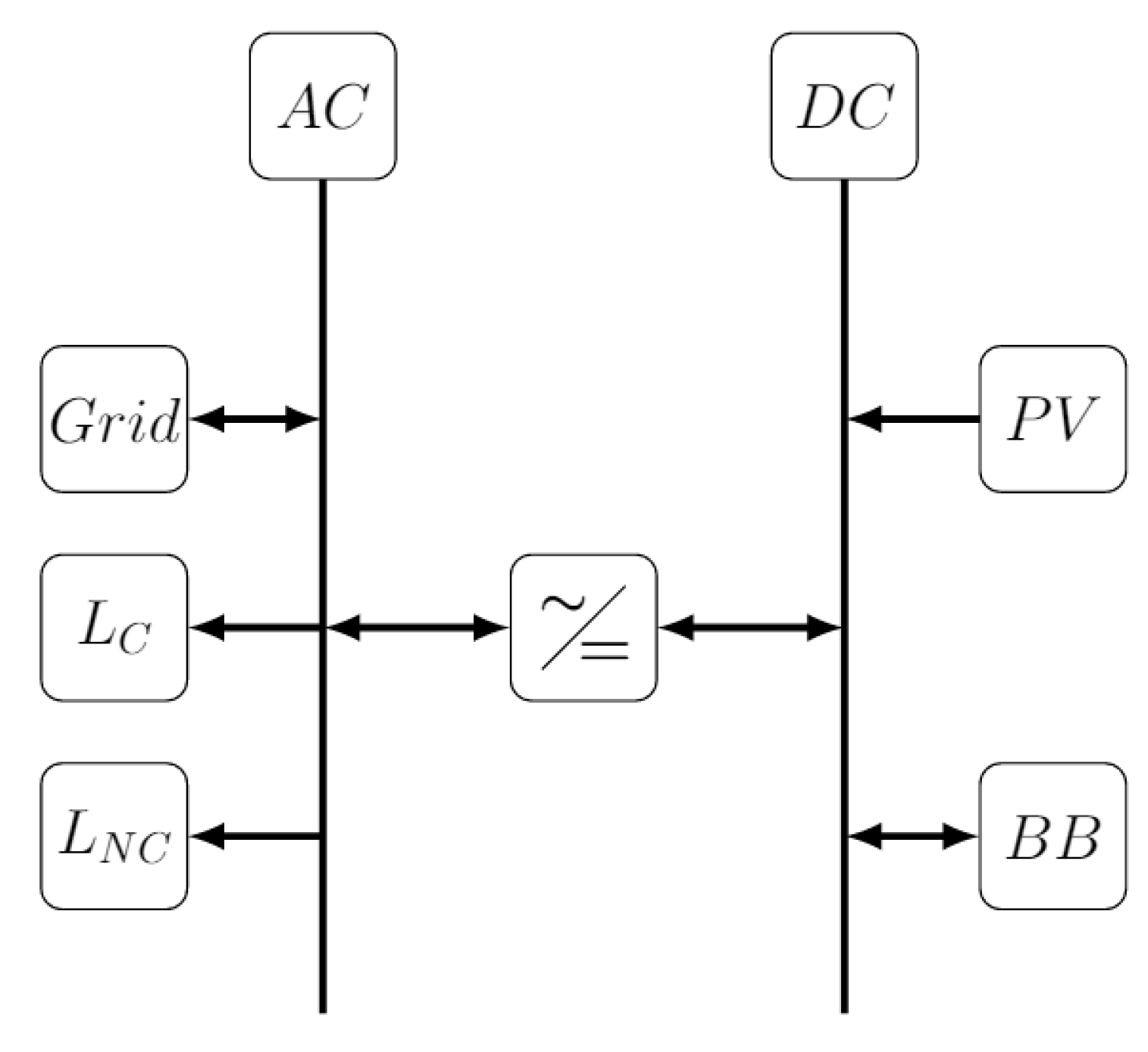
3.2. Energy Management System

The EMS based on the MPC approach drives the microgrid to minimize the following equation using a predicted horizon of N y = 48 h and a sampling time of 10 min:
min E i n , E o u t , B p , E c h , E d c h j = 0 N y 1 C i n · E i n ( k + j ) C o u t · E o u t ( k + j ) + j = 1 N y l = 1 N a g C l s t w · w l s t l ( k + j ) + C n s w · w n s l ( k + j )
The left side of Equation (12) specifies the minimization of costs for energy transactions with the distribution company at a price of C i n in $/kWh for purchases and C o u t in $/kWh for sales. The right side of Equation (12) seeks to minimize the water that was not supplied w n s l at a cost of C n s w in $/m 3 for N a g farmers as well as the lost water w l s t l due to excess irrigation at a cost of C l s t w in $/m 3 .
Among the constraints associated with the optimization problem is the energy balance given by:
E i n ( k + j ) + E p v ( k + j ) + E d c h ( k + j ) = E o u t ( k + j ) + E c h ( k + j ) + E p ( k + j ) + E n c ( k + j ) j = 1 N y
where E i n is the energy purchased from the distribution company, E p v denotes photovoltaic generation, E d c h denotes discharge from the battery bank, E o u t is the energy sold to the distribution company, E c h is the charge of the battery bank, E p denotes energy consumed by the water pumps, and E n c denotes the non-controllable load, which corresponds to domestic energy consumption by the community. Another relevant constraint is the maximum drop in the hydraulic threshold when pumping from well i to a height r, which is given by:
ε s ( r , t ( n ) ) = k = 0 n B p i ( k ) B p i ( k 1 ) · q b i 4 π T · W S r 2 4 T t ( n ) t ( k )
where B p i ( k ) is a binary decision variable for pumping into well i at instant k, q b i is the nominal flow of pump i in l/s, and r is the elevation to be pumped to, in m, considering that the worst case is less than the midpoint between the two closest wells. The control actions u ( k + j ) = { E i n , E o u t , B p , E c h , E d c h } are calculated based on the optimization problem defined by the objective function in Equation (12) and the constraints in Equations (13) and (14) at each sampling time, and the action at instant k is applied to the energy–water system. In the next time step, a new optimal control action is determined (rolling horizon). The 48-h-ahead predictions for electricity consumption and solar radiation, based on auto-regressive integrated moving average (ARIMA)-type models, are used for the EMS based on MPC.
GUROBI offers advanced methods for solving mixed integer linear programming problems through the YALMIP library [36]. The GUROBI tool solves the MPC optimization of the EMS with a linear programming method that uses a branch-and-bound algorithm.

3.3. Water Management System

The WMS is based on the MPC approach and considers a prediction horizon of N y = 28 days and a sampling time of one day. This WMS optimization gives the irrigation volumes that maximize the benefits expected from all N c crops for the N a g farmers over the prediction horizon of N y , with N c = g = 1 N a g N c , g :
max V ¯ r , c c = 1 N c B c · Y r , c ( k + N y )
c = 1 N c C ω c · g ( Y r , c ( k ) , ω c ) ,
s . t . Y r , c ( k + N y ) = Y r , c ( k 1 ) · i = k k + N y 1 K y , c ( i ) · 1 K s , c ( i ) 1 M i , c ,
Y r , c ( k ) = 1
K s , c ( k ) = { T A W ( k ) D r ( k ) T A W ( k ) R A W ( k ) if R A W ( k ) < D r ( k ) , 1         otherwise ,
D r ( k ) = D r ( k 1 ) P ( k ) + R O ( k ) 1 , 000 · V ¯ r , c ( k ) A c C R ( k ) + D P ( k ) + E T p ( k ) ,
D r ( 0 ) = 1.000 · ( θ F C θ 0 ) · Z r ( 0 ) ,
g ( Y r , c ( k ) , ω c ) = max 0 , ( ω c Y r , c ( k ) ) ,
where the first term of the objective function in Equation (15a) corresponds to the maximization of the relative benefits due to the relative yields Y r , c ( k + N y ) of the crops under a horizon of N y . The coefficient B c is the relative benefit, which includes the benefits of cultivation in the community and is equivalent to [20]:
B c = Y p , c P c A c ,
where Y p , c is the optimum yield of crop c in kg/ha, P c is the expected price of crop c in $/kg, and A c is the cultivated area in ha. These data are obtained from the Office of Agrarian Studies and Policies [27] and from reports of the Food and Agriculture Organization of the United Nations [34,37].
The second term of the objective function in Equation (15b) is the penalty for not meeting a minimum expected relative return of ω c on the crop, where C ω c is a high relative cost and g ( Y r , c ( k ) , ω c ) is a function that determines the gap needed to reach the minimum expected return ω c .
The following terms correspond to the restrictions of the WMS formulation. Equation (15c) is the expected relative return at the end of the horizon N y , where Y r , c ( k 1 ) is the relative yield at time k 1 , K y , c ( k ) is the sensitivity of crop c to the lack of water, K s , c ( k ) = E T a , c ( k ) E T p , c ( k ) is the ratio between the actual and potential evapotranspiration for crop c, and M i , c is the duration in days of the corresponding growth stage of crop c. The initial condition of the crop yield in Equation (15d) is equal to 1 (maximum value); Equation (15e) gives the ratio between the actual and potential evapotranspiration; Equations (15f) and (15g) calculate the root zone depletion and its initial condition, respectively; and Equation (15h) defines the penalty function g ( Y r , c ( k ) , ω c ) . Associated with these formulations is the constraint on the extraction of water for all c crops from the aquifer, which must be less than its recharge volume R:
c = 1 N c V ¯ r , c ( k ) R .
The optimization problem defined by the objective function in Equations (15a) and (15b) and the constraints in Equations (15c)–(15h), (16) and (17) provides the control action given by the required irrigation volumes at each sampling time (i.e., each day). In the next time step, a new optimal control action is determined (rolling horizon). The 28-days-ahead predictions for temperature, radiation, wind speed, and precipitation based on auto-regressive models are used for the WMS based on MPC.
To solve the WMS optimization problem we apply a genetic algorithm to the optimization variables, where each gene on the chromosome represents a daily irrigation volume for a culture V ¯ r , c ( k ) V ¯ r , c ( k + N y 1 ) over a prediction horizon of N y days. The number of chromosomes per individual is equal to the number of optimization variables of the problem:
N v a r = N c · N y ,
where N c is the total number of crops.
The next section shows the results of applying the proposed methodology to the selected case study.

4. Case Study

Although Chile has a high electrification rate (99.8% for 2017 [38]), it is estimated that 25,000 families are not connected to the electricity grid, while another 5000 only have a partial supply for a few hours a day [39]. Indeed, many isolated rural dwellings that are connected to the electricity grid do not have a reliable supply throughout the year because of both voltage drops due to the considerable distances from electrical substations and the corrosive characteristics of coastal areas. This limits the opportunities to develop these rural regions. Many of these rural communities depend on agriculture for their livelihoods; however, the effects of climate change are having negative impacts on traditional agriculture. Historically, artificial irrigation has not been required in southern Chile because rainfall is distributed throughout the year, but the 2010–2018 period broke this trend, being the driest on record with a rainfall deficit of 20–40% [26].
As a case study, we evaluate the proposed EWMS strategy using data extracted from the José Painecura Hueñalihuen community located in the municipality of Carahue, Chile. The local hydrogeology indicates the presence of limited aquifer potential due to the high variability of sediments and rocks [40]. Groundwater is poorly understood in the region and has only been monitored since 2013. The authorities have reported a significant increase in water rights used primarily for human and animal consumption (55%), water for irrigation (33%), water for industrial use (10%), and other uses (2%). Two principal aquifer levels have been identified: one is superficial (less than 20 m depth) and the other is deeper (more than 20 m). The wells in the shallow aquifer tend to dry out in summer or during periods of drought. Thus, groundwater is closely related to river flows (especially the shallow aquifer, where decreases in precipitation directly affect the river flow), which are the most accessible groundwater type [41].
Figure 3 shows the location of the community, with a mountainous coastal terrain in which the crops grow on the hills and the water must be pumped from the aquifers for irrigation.
This community has an inadequate electricity supply, which is reflected in a System Average Interruption Duration Index of 69.51 [h]. The average interruption in Chile is 12.17 [h] [42]. In the future, we hope to setup a microgrid (connected to the main grid) to benefit 44 families. This microgrid will have the following characteristics:
  • Photovoltaic Power Plant, 90 kWp.
  • Lead-acid Battery Bank, 43.2 kWh.
  • 0.25 kW and 1.1 m 3 /h centrifugal pumps at a hydraulic height of 14 m. One pump is assumed per farmer.
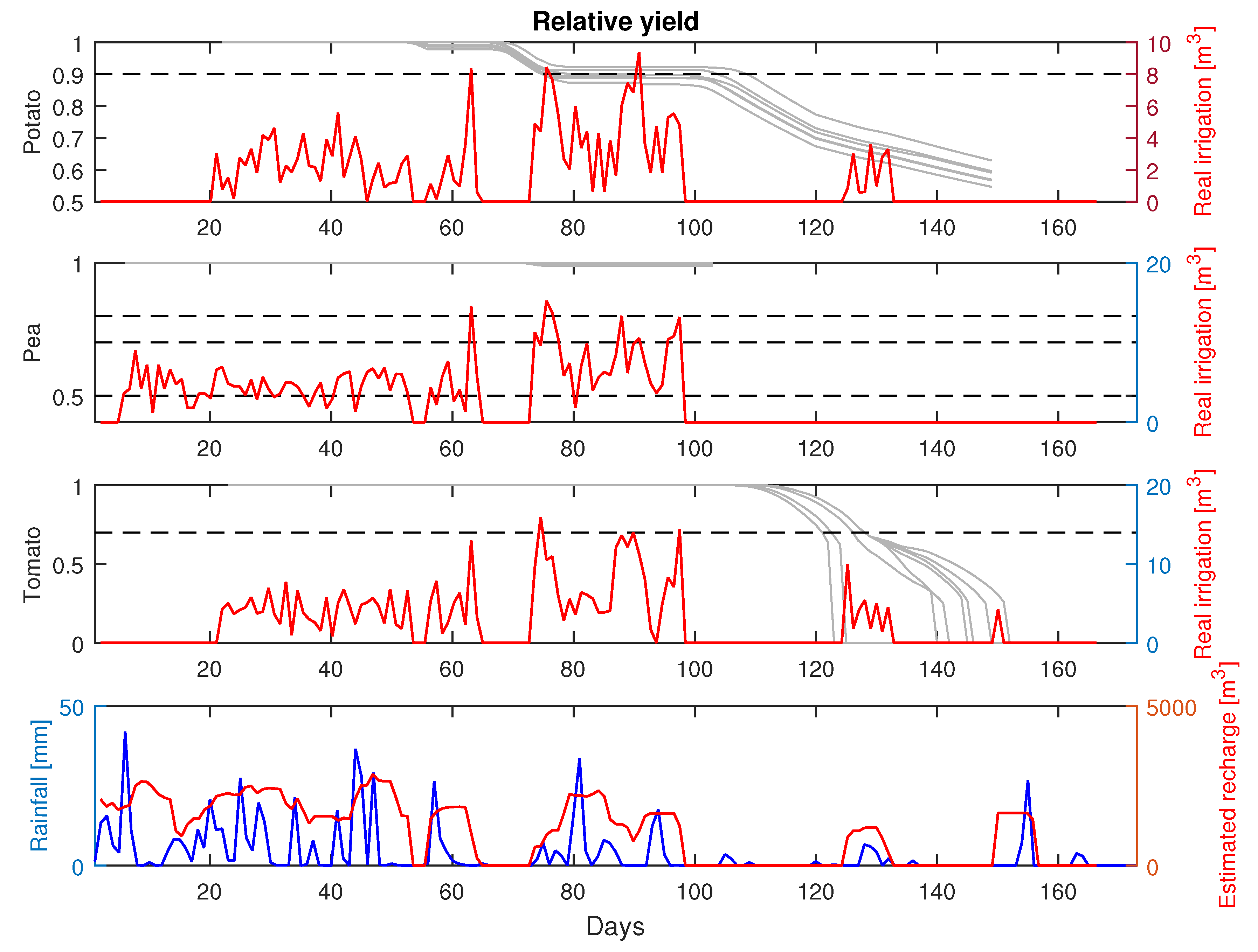
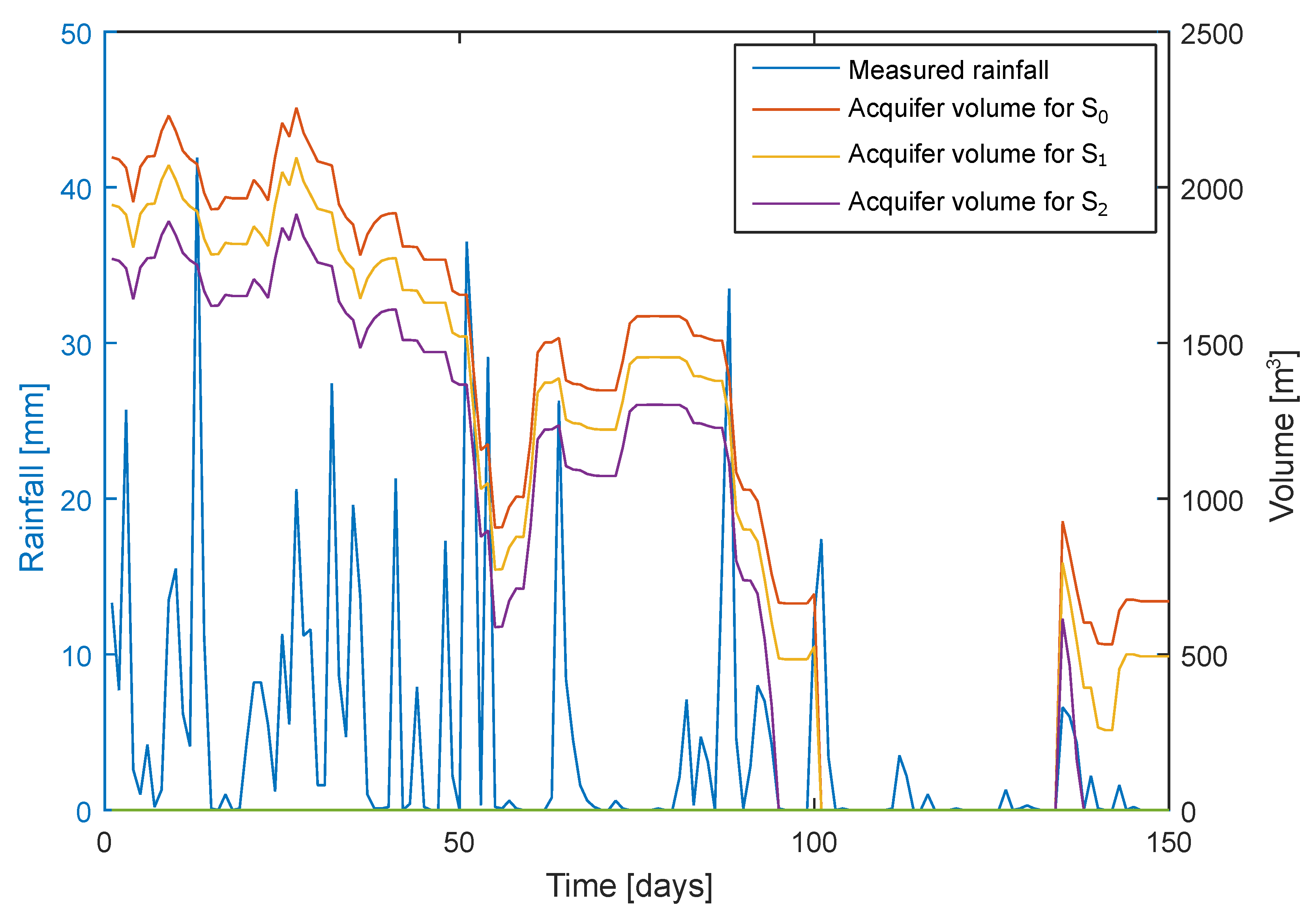
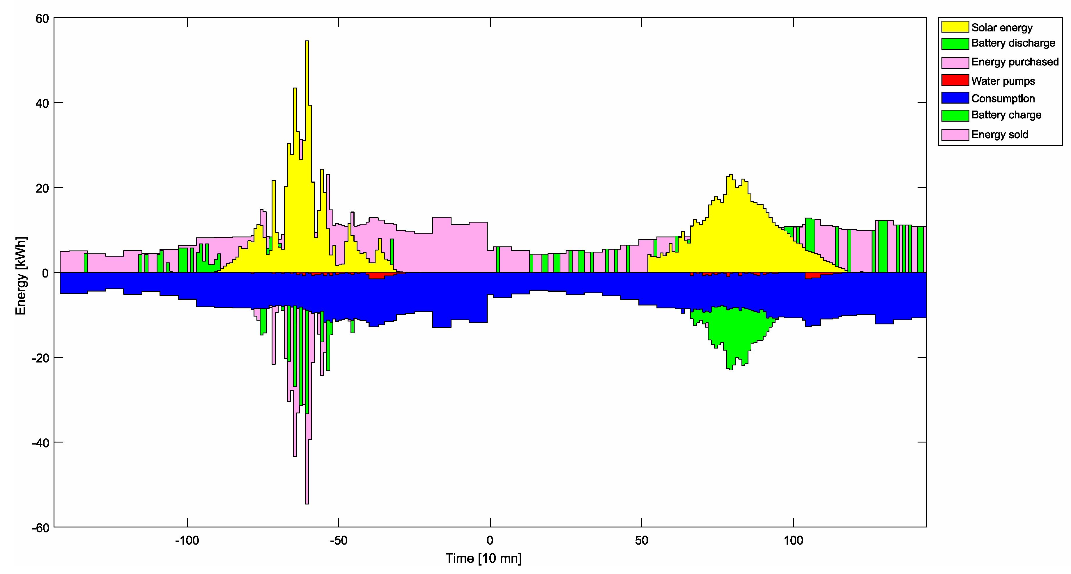
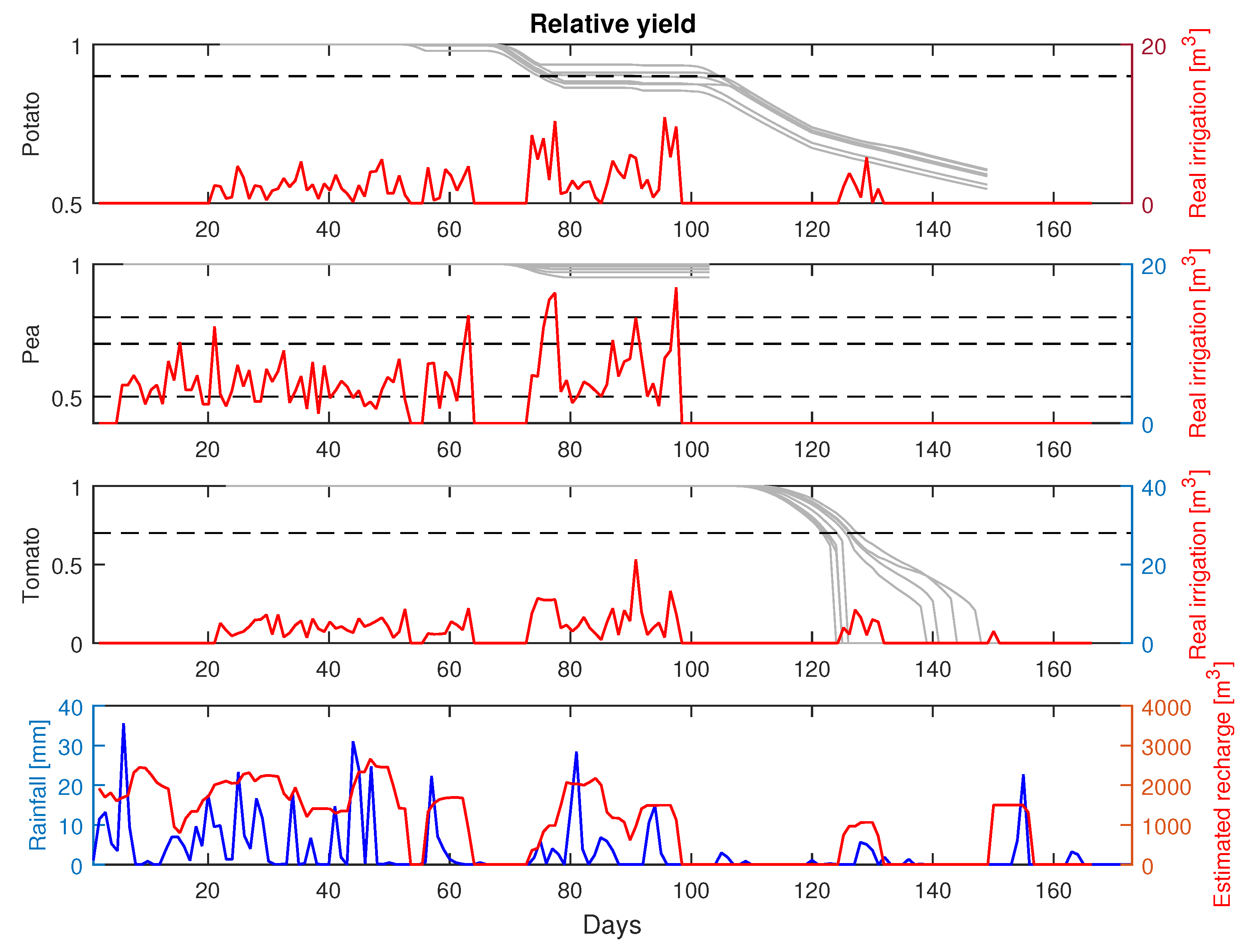
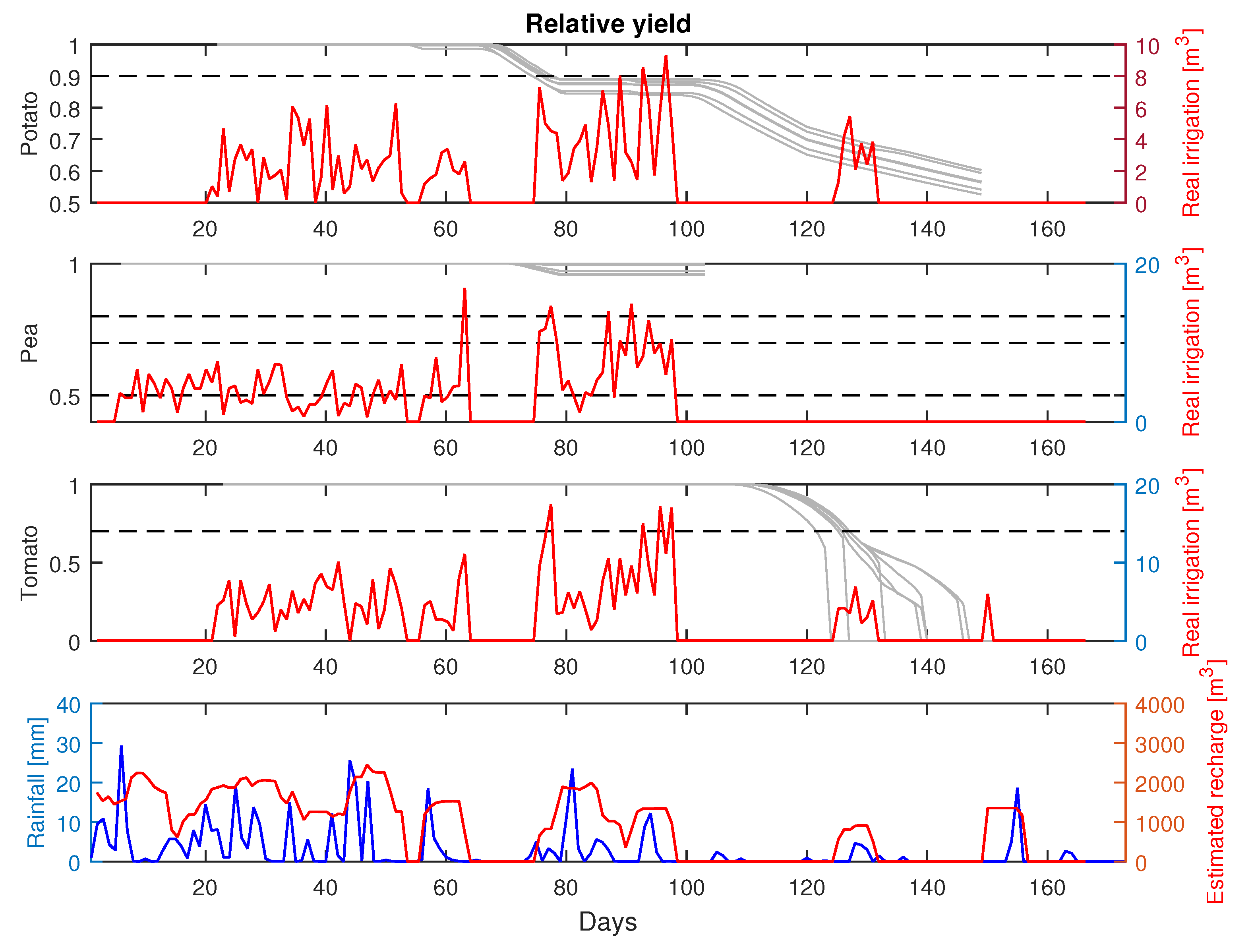
Figure 4 shows the microgrid topology. The controllable loads ( L C ), non-controllable loads ( L N C ), and the grid are identified in the AC bus, and the photovoltaic power plant ( P V ) and lead-acid battery bank ( B B ) are on the DC bus.
The crops present in the community are potatoes, peas, and tomatoes, whose main characteristics are expressed in Table 1. In the table, K y is the sensitivity to the lack of water at each stage, K c is a crop coefficient related to the growth stage, P c is a factor that relates the total water available in the root zone to the water that can be absorbed by the crop, and C N is the relative impermeability of the soil/vegetation. The sale price received by the farmers in Table 1 is approximated as half the final market price.
For the simulation, we considered ten farmers whose irrigation and pumping systems were managed by the EWMS system. Table 2 summarizes the two dominant parameters related to the three main crops cultivated by the farmers, which are the cultivated area and the minimum expected relative yield, Y m i n (related to the expected self-consumption).
We gathered temperature, solar radiation, and wind speed data from a meteorological station installed in the José Painecura Hueñalihuen community (38°32′11.1″ S, 73°30′12.9″ W), which recorded data at 10-min intervals between 5 July and 31 December 2015 (a total of 180 days). We used the General Water Directorate (DGA), which collects daily precipitation data at the millimeter-scale throughout Chile, to retrieve the rainfall data in the region of interest. For this study, we used the DGA:09153001 station located in Puerto Saavedra (38.7886 S, 73.3936 W, 5 m). We accessed the web page <http://explorador.cr2.cl> to retrieve historical weather data from DGA:09153001 covering the period 1 January 1979, to 11 December 2018. The data indicate a daily precipitation minimum of 0 mm, a maximum of 96.8 mm, and a daily average of 3.1 mm.
Finally, we set electronic devices to register the electricity consumption in 44 households in the community, namely those of the farmers included in this study [43]. We used ARIMA-type models with a prediction interval of two days for the short-term predictions. For the medium-term predictions, we used a moving average of the data over the past seven days, as obtained daily, based on the daily minimum and maximum values of temperature, average radiation, average wind speed, and precipitation. We used Equation (5) to estimate the aquifer recharge with a prediction interval of 28 days.
Figure 5 shows the rainfall for 150 days and the aquifer volume considering a baseline scenario ( S 0 ) and scenarios for decreases in rainfall of 15 and 30% ( S 1 and S 2 , respectively). The reductions were modeled by applying a multiplicative factor to the rainfall, which impacts the estimated aquifer recharge. Rainfall is expressed in mm and the influence area for aquifer recharge is 2.38 km 2 . The aquifer recharge is expressed in m 3 .

5. Results

Figure 6 shows two days of operations for the EWMS, where the generation and purchase of energy are seen in the positive semi-plane of the energy, while the consumption of the community, battery charging, and energy sale are along the negative axis. During the daytime, consumption is supplied primarily through photovoltaic generation, with excess energy stored in the battery bank. At night, power is supplied from the battery bank and through the purchase of energy.
The dispatch of pumps for water storage is generally distributed throughout the day, along with the excess photovoltaic energy. There is a concentration of pumping action at the end of the day, even though it is necessary to purchase power or discharge the battery bank. This is because the established schedule for irrigation and the capacity of the storage ponds often does not satisfy the daily water demand. Therefore, the EWMS must perform simultaneous pumping and irrigation.
Figure 7 shows the individual yields by crop type, minimum expected yields, and water availability based on the rainfall and aquifer recharge. The figure shows the dispatch for all pumps in compliance with the irrigation references using the proposed EWMS-based MPC. Before and immediately after the recharge of the aquifer is predicted to be insufficient, the WMS requires considerably more water for irrigation to cushion the effects of water scarcity on crops. It can be observed that when irrigation occurs, the WMS is useful at maintaining the relative crop yield. When insufficient irrigation causes a decrease in the relative yield, it is still useful in reducing the slope of the yield loss.
The pea crop has a higher yield than the established limit, as this crop is planted before the others and has 100 days between planting and harvesting. This avoids times during the year with lesser rainfall. Each period of low recharge impacts the relative crop yields, which eventually exhausts the available water that can be absorbed by the plants and results in a loss of yield or the death of the plant.
The scenarios with decreased rainfall of 15% and 30% ( S 1 and S 2 , respectively) are shown in Figure 8 and Figure 9. Scenarios S 1 and S 2 present similar irrigation actions to those of S 0 (normal rainfall). There is no irrigation when aquifer recharge is not expected based on the weather forecast. In both cases, similar final yields are observed for all crops, highlighting the lower yield of the pea for scenarios S 1 and S 2 relative to S 0 . The potato yield for scenario S 2 is slightly lower. This is explained by the lower rainfall and the consequent lower daily available water for extraction. The main differences occur in the daily irrigation peaks, which are lower with less rainfall because of the decreased daily water availability for extraction, as caused by the aquifer’s slow recharge. Table 3 lists the operational costs as computed using the EMS objective functions in Equation (12) and the profit obtained when computing the WMS objective functions with Equations (15a) and (15b), as well as the irrigation volumes, for all scenarios.
In the scenarios with decreased rainfall (less available water), the higher operating costs of the EMS indicate that the irrigation water requirements cannot be met, which generates high penalties in the objective function. Furthermore, the profit decreases with less rainfall because the crop yields also decrease. Table 3 indicates that scenarios S 1 and S 2 have lower water extractions from the aquifer, equivalent to 6% and 4.6%, respectively. Two simultaneous effects explain this: (i) lower rainfall contributions for the natural irrigation of crops, and (ii) less available water to extract from the aquifer. As there is reduced rainfall, the system tends to require more water from the wells; however, as there is less recharge of the aquifer, this extraction is limited.

6. Conclusions

This paper has described a novel design for the integrated management of energy and water as an EWMS for agriculture that employs a connected microgrid.
We have constructed the modules of the EWMS using an MPC approach based on phemonenological models with climate conditions in order to predict the impact of actions over a future horizon. In the medium term, with a prediction horizon of 28 days and a sampling time of one day, the WMS estimates optimal irrigation volumes for crops and transmits information to the EMS. The EMS dispatches the distributed energy resources in the short term, with a prediction horizon of 48 h and a sampling time of 10 min, to satisfy the pumping water requirements. Meteorological forecasts allow hardening constraints during droughts to avoid depleting the aquifer. In addition, pumping constraints limit reductions in the aquifer level. This strategy integrates the management of both resources and includes constraints that avoid affecting the neighboring wells in the community.
The EWMS was tested using real data from a rural community in southern Chile. The results show that not all crops meet the minimum requirements, as they are influenced by the presence of different precipitation levels. In periods when there is little rainfall, there is no aquifer recharge, so irrigation cannot be performed. If these periods occur at critical times during cultivation, the yield will be severely diminished, possibly leading to a loss of all production. The EWMS has the flexibility to include different crops and aquifers to search for the best economic return from the crop yields according to the available water and energy. This flexibility makes EWMS suitable for boosting the local economic development of isolated communities that have access to microgrids for power generation. The methodology developed in this study is intended to be applied to other communities with similar water issues requiring the optimization of the water-energy-food nexus. The implemented EWMS optimizer allows modifications and extensions, and we intend to apply it in a real case at the pilot scale.

Author Contributions

Project administration, D.S.; Conceptualization, T.R., D.S., C.M. and L.D.; Data curation, T.R.; Formal analysis, T.R., D.S., C.M. and L.D.; Investigation, T.R., D.S., C.M. and L.D.; Methodology, D.S., C.M. and L.D.; Validation, T.R. and L.D.; Visualization, T.R., D.S., C.M. and L.D.; Writing—original draft, T.R., D.S., C.M. and L.D.; Writing—review and editing, T.R., D.S., C.M. and L.D. All authors have read and agreed to the published version of the manuscript.

Funding

This research was funded by CONICYT/FONDECYT (grant number 1170683) “Robust Distributed Predictive Control Strategies for the Coordination of Hybrid AC and DC Microgrids,” the Instituto Sistemas Complejos de Ingeniería (ISCI) funded by ANID PIA BASAL (grant number AFB180003), the Solar Energy Research Center SERC-Chile funded by ANID/FONDAP (grant number 15110019), and the Centro de Excelencia en Geotermia de los Andes (CEGA) funded by ANID/FONDAP (grant number 15090013).

Conflicts of Interest

The authors declare no conflict of interest. The funders had no role in the design of the study; in the collection, analysis, or interpretation of data; in the writing of the manuscript; or in the decision to publish the results.

Abbreviations

The following abbreviations are used in this manuscript:
WMSWater Management System
EMSEnergy Management System
EWMSEnergy–Water Management System
MPCModel Predictive Control
HSHydrological System
DGAGeneral Water Directorate
TAWTotal Available Water
ARIMAAuto-Regressive Integrated Moving Average

References

  1. United Nations. World Population Prospects 2019: Wallchart; United Nations: New York, NY, USA, 2019; p. 2.
  2. Ferroukhi, R.; Nagpal, D.; Lopez-Peña, A.; Hodges, T.; Mohtar, R.H.; Daher, B.; Mohtar, S.; Keulertz, M. Renewable Energy in the Water, Energy and Food Nexus; International Renewable Energy Agency: Abu Dhabi, United Arab Emirates, 2015; pp. 1–125. [Google Scholar]
  3. Zhang, J.; Campana, P.E.; Yao, T.; Zhang, Y.; Lundblad, A.; Melton, F.; Yan, J. The water-food-energy nexus optimization approach to combat agricultural drought: A case study in the United States. Appl. Energy 2018, 227, 449–464. [Google Scholar] [CrossRef]
  4. Nhamo, L.; Ndlela, B.; Nhemachena, C.; Mabhaudhi, T.; Mpandeli, S.; Matchaya, G. The water-energy-food nexus: Climate risks and opportunities in Southern Africa. Water 2018, 10, 567. [Google Scholar] [CrossRef] [Green Version]
  5. Liu, Z.; Yang, J.; Jiang, W.; Wei, C.; Zhang, P.; Xu, J. Research on optimized energy scheduling of rural microgrid. Appl. Sci. 2019, 9, 4641. [Google Scholar] [CrossRef] [Green Version]
  6. Whitney, E.; Schnabel, W.E.; Aggarwal, S.; Huang, D.; Wies, R.W.; Karenzi, J.; Huntington, H.P.; Schmidt, J.I.; Dotson, A.D. MicroFEWs: A Food-Energy-Water Systems Approach to Renewable Energy Decisions in Islanded Microgrid Communities in Rural Alaska. Environ. Eng. Sci. 2019, 36, 843–849. [Google Scholar] [CrossRef] [Green Version]
  7. Alzola, J.A.; Camblong, H.; Niang, T. Promotion of Microgrids and Renewable Energy Sources for Electrification in Developing Countries; Technical Report; European Commission: Brussels, Belgium, 2008. [Google Scholar]
  8. Fornarelli, R.; Anda, M.; Louise, D.; Parisa, B. Conceptual model of energy and water micro-grid solutions with consumer engagement: An Australian case study. In Proceedings of the 10th International Conference on Water Sensitive Urban Design: Creating Water Sensitive Communities (WSUD 2018 & Hydropolis 2018), Perth, Australia, 13–15 February 2018; pp. 159–169. [Google Scholar]
  9. Zhang, X.; Sharma, R.; He, Y. Optimal energy management of a rural microgrid system using multi-objective optimization. In Proceedings of the 2012 IEEE PES Innovative Smart Grid Technologies (ISGT), Washington, DC, USA, 16–20 January 2012; IEEE: New York, NY, USA, 2012; pp. 1–8. [Google Scholar] [CrossRef]
  10. Michalski, J. Microgrids for Micro-Communities: Reducing the Energy Burden in Rural Areas. Mich. Technol. Law Rev. 2019, 26, 145–174. [Google Scholar] [CrossRef]
  11. Karan, E.; Asadi, S.; Mohtar, R.; Baawain, M. Towards the optimization of sustainable food-energy-water systems: A stochastic approach. J. Clean. Prod. 2018, 171, 662–674. [Google Scholar] [CrossRef]
  12. Chen, C.; Zeng, X.; Yu, L.; Huang, G.; Li, Y. Planning energy-water nexus systems based on a dual risk aversion optimization method under multiple uncertainties. J. Clean. Prod. 2020, 255, 120100. [Google Scholar] [CrossRef]
  13. Nikam, N.G.; Regulwar, D.G. Optimal Operation of Multipurpose Reservoir for Irrigation Planning with Conjunctive Use of Surface and Groundwater. J. Water Resour. Prot. 2015, 7, 636–646. [Google Scholar] [CrossRef] [Green Version]
  14. Mérida, A.; Gallagher, J.; McNabola, A.; Camacho, E.; Montesinos, P.; Rodríguez, J.A. Comparing the environmental and economic impacts of on- or off-grid solar photovoltaics with traditional energy sources for rural irrigation systems. Renew. Energy 2019, 140, 895–904. [Google Scholar] [CrossRef]
  15. Powell, J.W.; Welsh, J.M.; Farquharson, R. Investment analysis of solar energy in a hybrid diesel irrigation pumping system in New South Wales, Australia. J. Clean. Prod. 2019, 224, 444–454. [Google Scholar] [CrossRef]
  16. Labadie, J.W. Optimal Operation of Multireservoir Systems: State-of-the-Art Review. J. Water Resour. Plan. Manag. 2004, 130, 93–111. [Google Scholar] [CrossRef]
  17. William, W.G.Y. Reservoir Management and Operations Models. Water Resour. Res. 1985, 21, 1797–1818. [Google Scholar] [CrossRef]
  18. Brdys, M.A.; Grochowski, M.; Giminski, T.; Konarczak, K.; Drewa, M. Hierarchical predictive control of integrated wastewater treatment systems. Control Eng. Pract. 2008, 16, 751–767. [Google Scholar] [CrossRef]
  19. Vedula, S.; Nagesh Kumar, D. An integrated model for optimal reservoir operation for irrigation of multiple crops. Water Resour. Res. 1996, 32, 1101–1108. [Google Scholar] [CrossRef]
  20. Reddy, M.J.; Kumar, D.N. Optimal reservoir operation for irrigation of multiple crops using elitist-mutated particle swarm optimization. Hydrol. Sci. J. 2007, 52, 686–701. [Google Scholar] [CrossRef]
  21. Cai, X.; McKinney, D.C.; Lasdon, L.S. Integrated hydrologic-agronomic-economic model for river basin management. J. Water Resour. Plan. Manag. 2003, 129, 4–17. [Google Scholar] [CrossRef] [Green Version]
  22. Georgiou, P.E.; Papamichail, D.M. Optimization model of an irrigation reservoir for water allocation and crop planning under various weather conditions. Irrig. Sci. 2008, 26, 487–504. [Google Scholar] [CrossRef]
  23. Georgiou, P.E.; Papamichail, D.M.; Vougioukas, S.G. Optimal irrigation reservoir operation and simultaneous multi-crop cultivation area selection using simulated annealing. Irrig. Drain. 2006, 55, 129–144. [Google Scholar] [CrossRef]
  24. Famiglietti, J.S. The global groundwater crisis. Nat. Clim. Chang. 2014, 4, 945–948. [Google Scholar] [CrossRef]
  25. Vahid Pakdel, M.J.; Sohrabi, F.; Mohammadi-Ivatloo, B. Multi-objective optimization of energy and water management in networked hubs considering transactive energy. J. Clean. Prod. 2020, 266, 121936. [Google Scholar] [CrossRef]
  26. Garreaud, R.D.; Boisier, J.P.; Rondanelli, R.; Montecinos, A.; Sepúlveda, H.H.; Veloso-Aguila, D. The Central Chile Mega Drought (2010–2018): A climate dynamics perspective. Int. J. Climatol. 2020, 40, 421–439. [Google Scholar] [CrossRef]
  27. Información para el Desarrollo Productivo Ltda. (INFODEP). Elaboración de una Base Digital del Clima Comunal de Chile: Línea Base (1980–2010) y Proyección al Año 2050; Technical Report; Ministerio del Medio Ambiente: Santiago, Chile, 2016. [Google Scholar]
  28. Chai, J.; Shi, H.; Lu, Q.; Hu, Y. Quantifying and predicting the Water-Energy-Food-Economy-Society-Environment Nexus based on Bayesian networks—A case study of China. J. Clean. Prod. 2020, 256, 1–11. [Google Scholar] [CrossRef]
  29. Theis, C. The relation between the lowering of the Piezometric surface and the rate and duration of discharge of a well using ground-water storage. Eos Trans. Am. Geophys. Union 1935, 16, 519–524. [Google Scholar] [CrossRef]
  30. Raes, D.; Geerts, S.; Kipkorir, E.; Wellens, J.; Sahli, A. Simulation of yield decline as a result of water stress with a robust soil water balance model. Agric. Water Manag. 2006, 81, 335–357. [Google Scholar] [CrossRef]
  31. Jensen, M.E. Water consumption by agricultural plants. In Plant Water Consumption and Response. Water Deficits and Plant Growth; Kozlowski, T.T., Ed.; USDA: New York, NY, USA, 1968; Volume II, pp. 1–22. [Google Scholar]
  32. Monteith, J. Symposia of the Society for Experimental Biology. Yale J. Biol. Med. 1965, 25, 205–234. [Google Scholar]
  33. Doorenbos, J.; Bentvelsen, C.L.M.; Kassam, A.H.; Branscheid, V.; Bentvelsen, C.I.M. Yield Response to Water; FAO Irrigation and Drainage Paper; Food and Agriculture Organization of the United Nations: Rome, Italy, 1979; p. 193. [Google Scholar]
  34. Allen, R.; Pereira, L.; Raes, D.; Smith, M. Crop Evapotranspiration—Guidelines for Computing Crop Water Requirements; Technical Report; Food and Agriculture Organization of the United Nations: Rome, Italy, 1998. [Google Scholar]
  35. Camacho, E.F.; Bordons, C. Model Predictive Controllers, 2nd ed.; Springer: London, UK, 2007; p. 405. [Google Scholar] [CrossRef]
  36. Löfberg, J. YALMIP: A Toolbox for Modeling and Optimization in MATLAB. In Proceedings of the CACSD Conference, New Orleans, LA, USA, 2–4 September 2004. [Google Scholar]
  37. Smith, M.; Steduto, P. Yield Response to Water: The Original FAO Water; Technical Report; Food and Agriculture Organization of the United Nations: Rome, Italy, 2012. [Google Scholar]
  38. Ministerio de Desarrollo Social y Familia. CASEN 2017. Available online: http://datos.energiaabierta.cl/dataviews/256138/casen-2017-acceso-a-electricidad/ (accessed on 9 January 2020).
  39. Ministerio de Energía. Ruta de la Luz. 2019. Available online: https://www.energia.gob.cl/iniciativas/ruta-de-la-luz (accessed on 9 January 2020).
  40. Ciren, SitRural, Ministerio de Agricultura. Recursos Naturales, Comuna de Carahue; Technical Report; Ministerio de Agricultura: Santiago, Chile, 2018. [Google Scholar]
  41. Acevedo, P. Situación del Agua en la Araucanía. 2020. Available online: https://observatorio.cl/situacion-del-agua-en-la-araucania/ (accessed on 9 January 2020).
  42. Comisión Nacional de Energía. Electricidad—Energía Abierta. 2020. Available online: http://energiaabierta.cl/estadisticas/electricidad/?lang=en (accessed on 9 January 2020).
  43. Vargas, C.; Morales, R.; Sáez, D.; Hernández, R.; Muñoz, C.; Huircán, J.; Espina, E.; Alarcón, C.; Caquilpan, V.; Paine, N.; et al. Microgrid/Smart-Farm System: Case study applied to Indigenous Mapuche Communities. In Proceedings of the AACC’18 (The Second International Conference of ICT for Adapting Agriculture to Climate Change), Cali, Colombia, 21–23 November 2018; pp. 1–22. [Google Scholar]
Figure 1. Schematic of the hydrological system.
Applsci 10 07723 g001
Figure 2. Integrated EWMS model.
Applsci 10 07723 g002
Figure 3. Location of the José Painecura Hueñalihuen community [40].
Applsci 10 07723 g003
Figure 4. Topology of the proposed microgrid.
Applsci 10 07723 g004
Figure 5. Aquifer recharge estimation (m 3 ) for three scenarios: baseline scenario S 0 and scenarios S 1 and S 2 , which consider 15% and 30% decreases in rainfall, respectively. Measured rainfall (mm) for S 0 is also shown.
Applsci 10 07723 g005
Figure 6. EWMS operations for microgrids for the baseline scenario ( S 0 ).
Applsci 10 07723 g006
Figure 7. EWMS for crop yields, irrigation, rainfall, and estimated recharge for the baseline scenario ( S 0 ). The left y-axis in the potato, pea, and tomato plots indicates the relative yield of the different crops (gray) and their expected relative yields (dashed line), and the right y-axis indicates the irrigation (red). The fourth plot shows the measured rainfall (blue) and the estimated recharge (red).
Applsci 10 07723 g007
Figure 8. EWMS for crop yields, irrigation, rainfall, and estimated recharge for scenario 1 ( S 1 ). The left y-axis in the potato, pea, and tomato plots indicates the relative yield of the different crops (gray) and their expected relative yields (dashed line), and the right y-axis indicates the irrigation (red). The fourth plot shows the measured rainfall (blue) and the estimated recharge (red).
Applsci 10 07723 g008
Figure 9. EWMS for crop yields, irrigation, rainfall, and estimated recharge for scenario 2 ( S 2 ). The left y-axis in the potato, pea, and tomato plots indicates the relative yield of the different crops (gray) and their expected relative yields (dashed line), and the right y-axis indicates the irrigation (red). The fourth plot shows the measured rainfall (blue) and the estimated recharge (red).
Applsci 10 07723 g009
Table 1. Crop characteristics.
ParameterPotatoPeaTomato
Crop start31 July15 July1 August
Sale price [CLP/kg]280560220
Y m a x [kg/ha]31.7601.28086.910
Max height [m]0.60.50.9
Root depth [m]0.40.80.6
Stage duration [d][25,30,45,30][20,30,35,15][30,40,40,25]
K y [0.4,0.33,0.46,0.2][1,1,1,1][1,1,1,1]
K c [0.4,1.15,0.75][0.5,1.15,1.1][0.6,1.15,0.8]
P c 0.350.350.4
C N 706365
Table 2. Farmer crop characteristics.
PotatoPeaTomato
Area [m 2 ] Y min Area [m 2 ] Y min Area [m 2 ] Y min
A 1 5000.92500.8--
A 2 1.0000.95000.82500.7
A 3 --7500.81.0000.7
A 4 ----1250.7
A 5 2500.91250.51250.7
A 6 2500.92500.8--
A 7 2500.95000,81250.7
A 8 --7500.85000.7
A 9 ----1250,7
A 10 2500.95000.71250.7
Table 3. EWMS results using the baseline and reduced rainfall scenarios.
ScenarioCosts [ CLP ]Profit [ CLP ]Water Consumption [m 3 ]
S 0 : Normal rainfall120,34315141159.2
S 1 : Decreased rainfall of 15%127,13515111090.2
S 2 : Decreased rainfall of 30%140,84014671105.3
Publisher’s Note: MDPI stays neutral with regard to jurisdictional claims in published maps and institutional affiliations.

