Article

Evaluation of 32 Simple Equations against the Penman–Monteith Method to Estimate the Reference Evapotranspiration in the Hexi Corridor, Northwest China

1
Key Laboratory of Eco-hydrology of Inland River Basin, The Northwest Institute of Eco-Environment and Resources, Chinese Academy of Sciences (CAS), Lanzhou 730000, China
2
Northwest Institute of Eco-Environment and Resources, University of Chinese Academy of Sciences, Beijing 100049, China
3
Qilian Mountains Eco-Environment Research Center in Gansu Province, Lanzhou 730000, China
*
Author to whom correspondence should be addressed.
Water 2020, 12(10), 2772; https://doi.org/10.3390/w12102772
Submission received: 1 August 2020 / Revised: 28 September 2020 / Accepted: 30 September 2020 / Published: 5 October 2020
(This article belongs to the Section Water, Agriculture and Aquaculture)

Abstract

:
Evapotranspiration plays an inevitable role in various fields of hydrology and agriculture. Reference evapotranspiration (ET0) is mostly applied in irrigation planning and monitoring. An accurate estimation of ET0 contributes to decision and policymaking processes governing water resource management, efficiency, and productivity. Direct measurements of ET0, however, are difficult to achieve, often requiring empirical methods. The Penman–Monteith FAO56 (PM-FAO56) method, for example, is still considered to be the best way of estimating ET0 in most regions of the globe. However, it requires a large number of meteorological variables, often restricting its applicability in regions with poor or missing meteorological observations. Furthermore, the objectivity of some elements of the empirical equations often used can be highly variable from region to region. The result is a need to find an alternative, objective method that can more accurately estimate ET0 in regions of interest. This study was conducted in the Hexi corridor, Northwest China. In it we aimed to evaluate the applicability of 32 simple empirical ET0 models designed under different climatic conditions with different data inputs requirements. The models evaluated in this study are classified into three types of methods based on temperature, solar radiation, and mass transfer. The performance of 32 simple equations compared to the PM-FAO56 model is evaluated based on model evaluation techniques including root mean square error (RMSE), mean absolute error (MAE), percentage bias (PBIAS), and Nash–Sutcliffe efficiency (NSE). The results show that the World Meteorological Organization (WMO) and the Mahringer (MAHR) models perform well and are ranked as the best alternative methods to estimate daily and monthly ET0 in the Hexi corridor. The WMO and MAHR performed well with monthly mean RMSE = 0.46 mm and 0.56 mm, PBIAS = 12.1% and −11.0%, and NSE = 0.93 and 0.93, before calibration, respectively. After calibration, both models showed significant improvements with approximately equal PBIAS of −2.5%, NSE = 0.99, and RMSE of 0.24 m. Calibration also significantly reduced the PBIAS of the Romanenko (ROM) method by 82.12% and increased the NSE by 16.7%.

1. Introduction

Reference evapotranspiration (ET0) is an essential element of the hydrological cycle, energy, and water balance [1,2]. It plays a crucial role in the fields of agricultural and hydrological projects [3,4]. An accurate estimation of ET0 is a hydrological requirement for accurate estimates of water resource management, efficiency, and productivity, particularly in semi-arid regions [5,6].
The lysimetric method is one of the micrometeorological techniques used to measure in situ ET0 values, and it is often considered the sole method of achieving accurate ET0 estimates. This method, however, has great shortcomings associated with high costs and complex instrumentation [7,8]. A variety of empirical methods have thus been developed for the task according to different climate conditions [9,10,11,12].
The Food and Agriculture Organization (FAO) has recommended the Penman–Monteith (PM-FAO56) equation as the standard model to estimate the ET0 under various climate conditions and different time scales [13,14]. Research has shown the PM-FAO56 method to be suitable for a variety of climates with differing local factors. These include solar radiation, sunshine duration, wind speed, air humidity, air temperature, and location of observing station properties [15,16,17]. The model, however, requires a very large number of inputs, many of which are difficult to accurately estimate or observe in regions with few observations, such as those of wind speed, relative humidity, and solar radiation. A requirement to develop possible alternatives to escape some of these requirements could thus yield benefits in the development of the method [5,7,18,19,20].
The FAO also recommends an application of the Hargreaves and Samani (H-S) method of estimating ET0 values in regions where only observations of minimum and maximum air temperature [12] are available. However, many studies have found that the H-S method encounters uncertainties associated with regional climate conditions and small timescales [6,18]. Calibration of its inputs is therefore required before the method can be used reliably [6,18]. In light of these drawbacks, extensive research has been carried out to develop alternative, more simple equivalent methods [6,7,8,19,20,21].
Simple empirical ET0 models that use fewer climatic variables than those required by PM-FAO56 have been developed and showed relatively good performance [22]. Although not all models are synchronously applicable in all different regions, local calibration is indeed applied to reparametrize and adjust the model to local climate conditions [18,23,24].
Berti et al. (2014) [6] evaluated the performance of the H-S method in Italy and concluded that the H-S model overestimates ET0 values. Similar conclusions were obtained in Eastern North Carolina, America [25], Southeast Europe [21], and in Southwest China [26]. Significant improvements in H-S model performance in different regions have been gained through local calibration [6,18,23,26,27,28,29,30].
Gao et al. (2017) [31] evaluated different ET0 methods in arid, semiarid, and humid regions. They recommended the Priestly–Taylor, H-S, and Makkink models as the best substitutes for the PM-FAO56 model in arid, semi-arid, and humid regions of China, respectively [31,32,33]. The comparative studies of the performance of different simple ET0 models have been conducted in different regions of China [32,33,34,35,36,37,38,39,40,41]. Song et al. (2019) assessed the performance of twelve simple ET0 models in Northeast China during growing seasons and recommended the Valiantzas [42], Romanenko [43], and Makkink [44] models as substitutes for the PM-FAO56 [40]. An assessment of ten simple ET0 models based on local climates in China found the Berit et al. (2014) [6] method to be the best PM-FAO56 alternative for China [39]. Two other models (Turk [45] and Valiantzas [46]) were also found to give robust results in subtropical humid, monsoonal regions of China, although caveats persisted [31,37], particularly regarding evaluation and calibration. The current study aimed to evaluate the performance of 32 simple ET0 models in the arid region of the Hexi Corridor, Northwest China. This work is an additional key to further understanding the modeling of reference evapotranspiration and water resource management in inland river basins.

2. Study Area, Materials and Methods

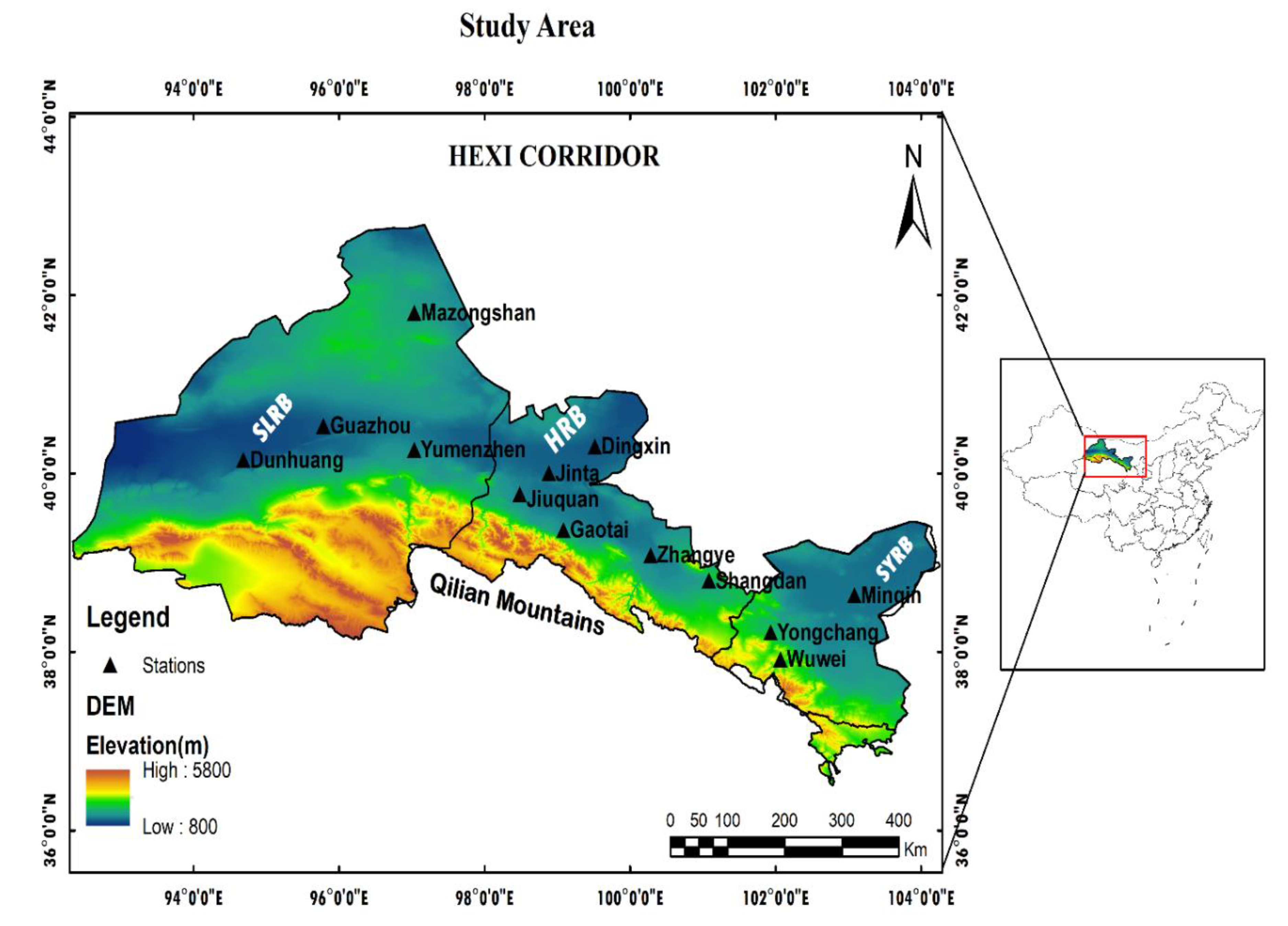
2.1. Geography and Climate of the Hexi Corridor

The elongated Hexi corridor is geographically situated between the latitudes 37°17′ N and 42°48′ N and longitudes 92°12′ E and 104°20′ E with an elevation of 800–5800 m (Figure 1). The corridor in Gansu province, China, is bounded by the Qilian Mountains to the south, and Mazong, Heli, and Longshou to the north extending from the Wushaoling mountain in the East to the Yumenguan in the west, and connects Northwest China to Xinjiang province. The area covered is 2.7 × 10⁵ km2, and is approximately 11.5% of the northwest region [47,48,49]. The corridor is primarily known as the source of dust in the Chinese loess [50]. It is also a major source of China’s wheat supply [51], as well as millet and corn [51,52]. Irrigation is essential due to low annual average precipitation in the region, as the result of a dominant westerly wind. The annual mean rainfall fluctuates between 50 and 550 mm [49]. Regional agriculture is found in oases distributed in three inland river basins, namely the Shiyang river basin (SYRB), Heihe river basin (HRB), and Shule river basin (SLRB), named after the three inland rivers located in the region, whose sources are in Qilian mountains. Moreover, the Hexi corridor has a high annual atmospheric water demand averaging from 1500 to 2500 mm [53].

2.2. Data and Source of Materials

Data used in this study were collected from thirteen meteorological stations distributed across the Hexi corridor (Figure 1). Daily observations were provided by the China Meteorological Administration (CMA) and include minimum, mean, and maximum air temperature (Tmin, Tmean, and Tmax), minimum and mean relative humidity (Rhmin and Rhmean), wind speed measured at 10 m height (U10m), and sunshine duration (SSD) for the period 1960–2017. Wind speeds, measured at 10 m height (also from CMA) and an assumed wind profile relationship were used to estimate mean values of wind speeds at 2 m height [12]. Maximum relative humidity (Rhmax) was estimated from mean and minimum relative humidity. Solar radiation (Rs) was estimated from sunshine duration (SSD) using Equation (37). Table 1 shows the properties of thirteen meteorological stations used in this study and summarizes the monthly means of the main climatic variables of each station in the Hexi corridor, observed during 1960–2017.

3. Methods and Methodology

3.1. Penman–Monteith Method

The FAO recommends the Penman–Monteith (FAO-PM56) method to estimate the daily ET0 from climatic variables [12], as shown in Equation (1):
E T 0 = 0.408 Δ ( R n G ) + γ 900 T m e a n + 273 u 2 ( e s e a ) Δ + γ ( 1 + 0.34 u 2 )
where E T 0 is the reference evapotranspiration (mm day−1), R n is net surface radiation, T m e a n is the average air temperature at 2 m height (°C), u 2 is the wind speed at 2 m height (m s−1), and ( e s e a ) is the saturation vapor pressure (kPa). The slope of the saturated vapor–vapor pressure curve (kPa °C) is Δ γ is the psychrometric constant, G is soil heat flux (MJ m−2 day−1), and e s and e a represent actual and saturation vapor pressure (kPa), respectively.

3.2. Simple ET0 Equations

To evaluate suitable, alternative methods to PM-FAO56, requiring fewer inputs while retaining results suitable for the Hexi corridor, this study selected 32 simple ET0 equations, classified into three categories: (1) temperature-based [6,7,8,19,43,54,55], (2) solar radiation-based [18,55,56,57,58,59], and (3) mass transfer-based [60,61,62]. The temperature-based methods are the most widely used to estimate the ET0 due to their relative simplicity and requirements of fewer inputs [63]. The radiation-based methods are also mostly used to estimate the ET0 at the global and regional scales. This study has also evaluated the performance of mass transfer methods compared to the PM-FAO56 method. The mass transfer (aerodynamic)-based methods are pioneers of empirical models to estimate evapotranspiration and originate from the method proposed by Dalton (1802) [62]. Previous studies showed that the mass transfer methods are built on the concept of eddy motion transfer of water vapor from the evaporating surface to the atmosphere [63,64]. Table 2 lists the ET0 models used in this study and their respective data requirements.
The ground heat flux at a daily time scale is ignored ( G = 0.0 ), whereas at a monthly time scale, G is delivered from monthly mean temperature [54].
G m = 0.14 ( T m T m 1 )
where m and m 1 are the month order.
The net surface radiation ( R n ) is obtained from the difference between the net short radiation ( R n s ) and the net long radiation ( R n l ) and expressed in Equation (35) below:
R n = R n s R n l
The net short radiation ( R n s ) is deduced from the surface albedo ( α 0.23 ) and solar radiation ( R s ) shown in Equation (36):
R n s = ( 1 α ) R s
As a direct measurement is missing, the solar radiation is derived from sunshine duration using the Hargreaves method shown in Equation (37) [12,22]. This method has been widely used in numerous studies conducted in Northwest China and showed a good agreement with available observations [39].
R s = R a × ( a s + b s n N )
where n is sunshine duration and N is maximum daylight hours; both variables are expressed in hours. a s and b s are Angstrom parameters, the PM-FAO56 assumes a s = 0.25 and b s = 0.50 , R s and R a are solar (shortwave) and extraterrestrial radiation, respectively, expressed in [MJm−2 day−1].

3.3. Model Evaluation, Selection, and Calibration

The performance of simple ET0 equations to estimate the daily and monthly ET0 values in the Hexi region was assessed through model evaluation techniques based on evaluating errors and regression metrics.
Error indices are among the regression metrics commonly used to evaluate models. In this study we selected mean absolute error (MAE) and root mean square error (RMSE) to compare errors between ET0 estimated from the PM-FAO56 method and that computed from simple ET0 equations. For both indices, values close to 0 were taken to be a measure of perfect model performance, similar to an approach taken by Singh et al. (2004) [72,73]. The linear regression coefficient (slope) was also used to indicate how well the ET0 values computed from simple models match the ET0 values estimated from the PM-FAO56 method. The regression metrics were also extended to the coefficient of determination (R2) to indicate the degree of agreement.
We also used the Nash–Sutcliffe efficient (NSE) method to evaluate the degree of fit between the PM-FAO56 method and the simple ET0 models. The NSE coefficients range between - and 1.0 with an optimum value of 1.0. Models with an NSE ranging between 0.0 and 1.0 can be considered for further model performance analysis, while models with NSE values 0.0 are considered to have unacceptable performance. Moriasi (2007) suggested a classification of model performance as follows: poor performance for models with N S E 0.50 , satisfactory for models with 0.50 < N S E 0.65 , good for models with 0.65 < N S E 0.75 , and very good for models with N S E > 75 [73]. Percentage bias (PBIAS) was adopted to explain the percentage of errors associated with model performance. PBIAS = 0% is an optimal value for the best model. A negative or positive sign indicates that the model overestimates or underestimates the ET0 values, respectively.
The formulation of the slope, MAE, RMSE, NSE, and PBIAS metrics are as follows:
M A E = 1 n i = 0 n 1 | E T i p m E T i e q |
R M S E = 1 n i = 0 n 1 ( E T i p m E T i e q ) 2
N S E = 1 [ i = 1 n ( E T i p m E T i e q ) 2 i = 1 n ( E T i p m E T m e a n p m ) 2 ]
P B I A S = [ i = 1 n ( E T i p m E T i e q ) i = 1 n E T i p m × 100 ]
where E T m e a n p m is the mean calculated as follows: E T m e a n p m = 1 n i = 1 n E T i p m . E T i p m and E T i e q both represent ET0 estimated at the ith day from the PM-FAO56 (pm) equation and simple ET0 equation (eq), respectively.
Based on evaluation metrics, the selected models were further calibrated. Similarly to the previous studies, this study used the regression-based with an omitted intercept method [74,75,76] to calibrate each selected model. The calibration process follows the following expression:
E T 0 p m = ψ E T 0 e q
The coefficient ψ stands for the linear regression coefficient estimated from the ratio E T 0 p m / E T 0 e q according to Xu and Sigh (1998) [65]. The time series of 1960–2017 was divided into two parts: 80% of the time series (1960–1999) was used to compute the ψ coefficient, and 20% of the time series (2000–2017) was used to validate the ET0 models. The calibration process relies on turning the constant values of the models in order to enhance their performances [76,77]. For each model, a constant value is changed to maximize the NSE and minimize the MAE, RMSE, and PBIAS. The results from the calibration procedure were assessed by the evaluation metrics (MAE, RMSE, PBIAS, and NSE) used in this study. The values of the ψ coefficient were calculated from the calibration data, and then the obtained ψ values were adopted for the testing and validation time series [75].

4. Results and Discussions

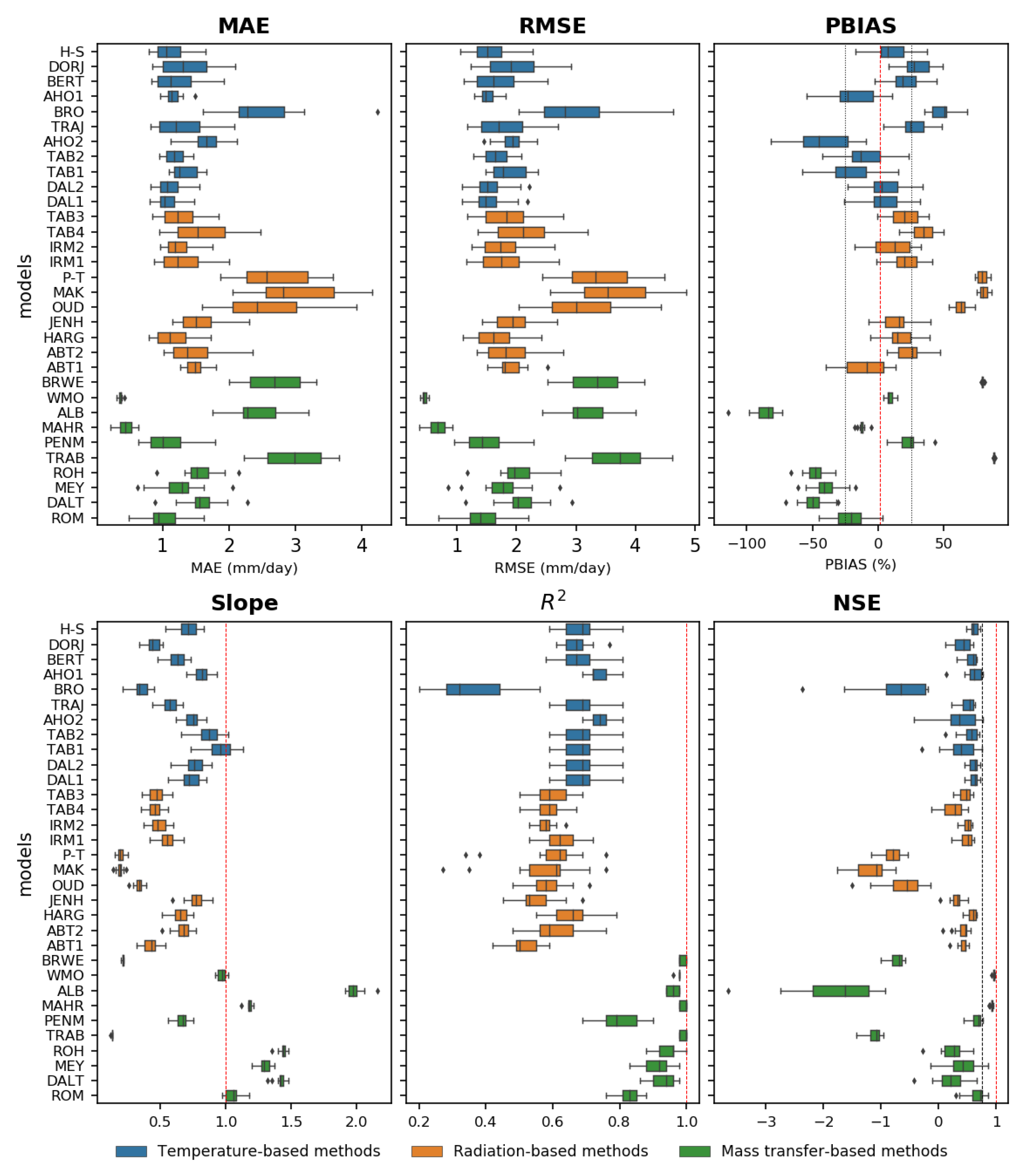
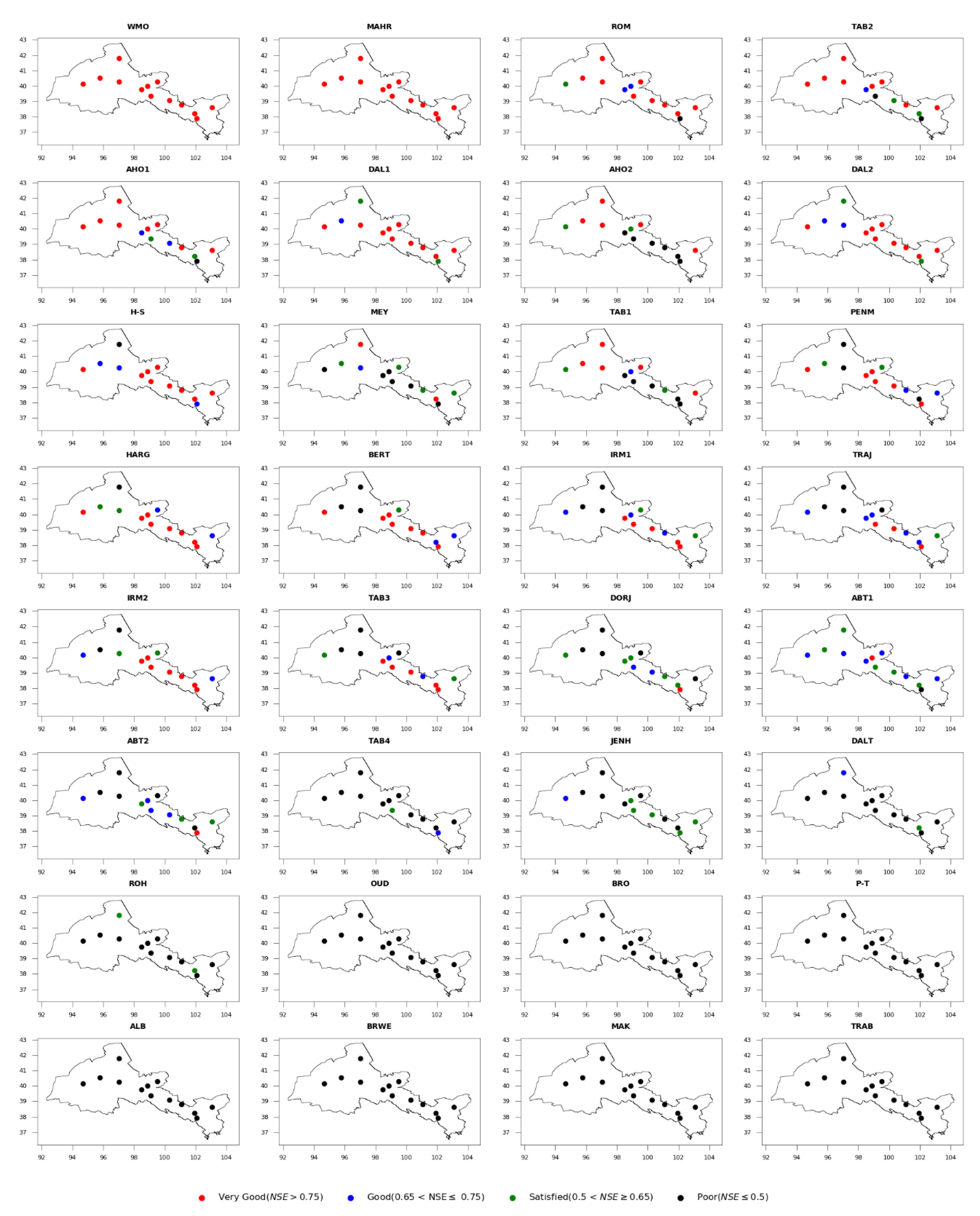
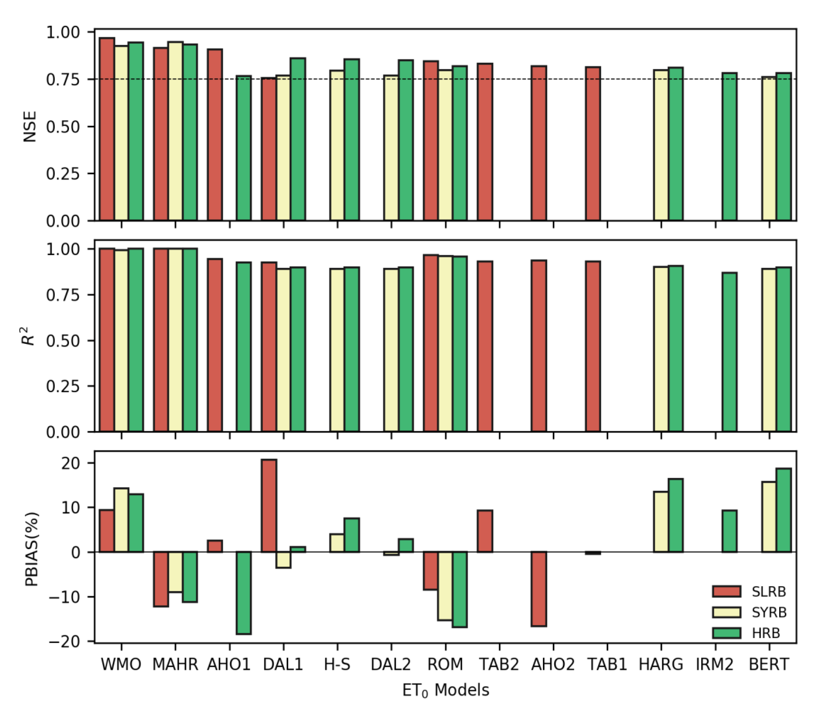
4.1. Performance of the Simple ET0 Models

Statistical metrics for the Hexi corridor obtained from comparisons between ET0 calculated from PM-FAO56 and 32 alternatives are shown in Figure 2 and Figure 3 for daily and monthly timescales, respectively. The MAHR and WMO models appear to show very good performance at all stations in the region. Figure 2 shows that both models estimated the daily ET0 values with relatively low MAE, RMSE, PBIAS, and significant NSE coefficients (Figure 2). On a daily basis, the WMO showed a relatively low range of MAE and RMSE bounded between 0.31–0.43 and 0.39–0.53 mm/day, respectively, and the MAHR showed low MAE, and RMSE in the ranges of 0.22–0.64 and 0.37–0.93 mm/day, respectively. Both models presented high NSE, and R2 values varied in the range of 0.88–0.98 and 98.0–1.0, respectively (Figure 2). On a monthly basis, the MAHR model gave small MAE values ranging between 0.15 and 0.63 mm and RMSE values ranging from 0.23 to 0.86 mm. It also resulted in PBIAS and NSE values averaged between −11% and 0.93%, respectively. The WMO also presented small MAE and RMSE values ranging from 0.38 to 0.53 mm and 0.35 to 0.45 mm, respectively, with an average PBIAS of 12% and an NSE of 0.95.
The mass transfer-based methods showed relatively higher slope- and R-squared (R2) with large and negative PBIAS values compared to other methods. The greater slope values and negative PBIAS values reveal the significant overestimations of the ET0 values estimated from the mass transfer methods on daily and monthly timescales, respectively. The ALB method showed an extreme overestimation of the ET0 values with a daily mean PBIAS of −86.7% and a monthly mean PBIAS of −88.4%. The DALT, ROH, MEY, and ROM methods overestimated the daily and monthly ET0 values by daily mean PBIAS values averaged to −49.1%, −48.2%, −39.5% and −22.1%, respectively, and monthly mean PBIAS values of −42.7%, −42.1%, −33.6%, −13.6%, respectively. However, some mass transfer methods, such as TRAB, BRWE, and PENM, underestimated the ET0 values, with mean PBIAS values of 87.7%, 78.8%, and 19% for the daily timescale and 88.1%, 79.53%, and 25.8% for monthly the timescale, respectively.
The comparison between the PM-FAO56 and radiation-based methods showed that the selected models generally underestimated the daily ET0, except for the ABT1 model. An underestimation of ET0 estimates from radiation-based models is shown by the large and positive daily and monthly mean values of PBSIAS ranging from 5.0% to 78.6% and 13.5% to 80.4%, respectively. Moreover, the solar radiation-based methods encountered higher mean values of MSE and RMSE (Figure 2 and Figure 3, respectively). The OUD, P-T, and MAK models strongly underestimated the daily ET0 by the mean PBIAS of 38.4%, 59.6%, and 77.1%, respectively (Figure 2). Those models also underestimated the monthly ET0 values by 64.6%, 80.4%, 81.3%, respectively. The P-T and MAK methods used in this study were originally developed for a humid climate. They are significant for a 10 days or longer timescale, which may be the reason of their poor performance in the arid region [78]. Moreover, Tabari et al. (2011) showed that P-T underestimates the ET0 in cold and arid regions [18]. By contrast, the ABT1 model overestimated the daily ET0 values with a mean PBIAS of −14.9% and monthly ET0 values with a mean PBIAS of −6.5%.
The temperature-based methods showed relatively lower mean MAE and RMSE values than those estimated from the solar radiation and mass transfer-based methods. The daily and monthly mean MAE values estimated between the PM-FAO56 and temperature models are in the range of 0.48–6.6 mm/day and 0.41–4.5 mm, respectively. The daily and monthly mean RMSE values also vary in the range of 0.65–6.9 mm/day and 0.5–4.6 mm, respectively. However, the BRO method underestimated the ET0 values with the highest daily and monthly mean MAE and RMSE average to 2.7 and 3.2 mm/day and 2.6 and 2.8 mm, respectively, which led this model to perform with the lowest R2 and NSE values (Figure 2 and Figure 3). The poor performance is due to the extreme values observed during the freezing period (December–April) [22]. It has been shown that the temperature-based methods are more sensitive to weather conditions and the BRO method showed to perform well under a temperature range of 11–22.5 °C [20]. Other temperature-based methods underestimated the daily and monthly ET0 values, including BERT, DORJ, and TRAJ, with the mean PBIAS ranging between 19.8% and 47.9% (Figure 2). The method proposed by Berti et al. (2014) underestimated the ET0 values with mean a PBIAS of 19.8% and 22.9% on a daily and monthly basis, respectively. Moreover, the strong underestimation of the daily and monthly ET0 values was estimated at the Mazongshan station with a PBIAS of 44.7% and 46.8%, respectively. The DAL1 and DAL2 methods showed good performance with a relatively lower daily mean PBIAS of −0.34% and 1.9% at and monthly mean PBIAS of 6.1% and 7.9%, respectively. Moreover, the large number of temperature-based models presented the greater slope and R2 values than that which resulted from the solar radiation methods (Figure 2 and Figure 3).
Figure 4 and Figure 5 show the spatial distribution of NSE values in the Hexi corridor. In both Figures, the WMO and MAHR models are robust at all weather stations. They present daily NSE values that vary from 0.71 to 0.99 and monthly NSE values ranging from 0.87 to 0.98.
From Figure 4, the selected temperature-based models showed mixed results, dominated by good and satisfactory performances. The AHO1, AHO2, and TAB1 models showed a very good performance with NSE = 0.78, 0.78, and 0.76 at Mazongshan station, respectively. Moreover, the AHO1 model also performed well at Yumenzhen station with NSE = 0.76 and showed a good performance at Dingxin, Guazhou, and Minqin. The DAL1, DAL2, and H-S models showed satisfactory performance with average NSE values of 0.65, 0.64, and 0.65, respectively, in the middle reach of the Heihe river basin. Moreover, the H-S method showed poor performance at Mazongshan and Guazhou stations while both DAL1 and DAL2 performed poorly at Wuwei station with N S E 0.50 . The low performance in these three models is associated with underestimating the daily ET0 at a large number of stations in the Hexi corridor. The solar radiation-based methods showed a relatively low performance compared to temperature-based and mass transfer-based methods. The HARG, IRM1, IRM2, and TAB3 models showed satisfactory performance in the Heihe river basin (Figure 4).
Figure 5 shows that most ET0 models are robust on the large timescale. The ROM model [43] showed a robust performance at more than 80% of the stations in the Hexi corridor (Figure 5). Among the temperature-based methods, the TAB2, AHO1, H-S, DAL2, and DAL1 models showed a significant performance compared to their corresponding daily values. The DAL1 showed a good estimate of the monthly ET0 with a RMSE averaged to 0.89 mm and a relatively high performance (NSE = 0.81), while TAB2 and AHO1 performed well in the Shule river basin. In general, significant improvements were observed in a large number of temperature-based methods, concentrated in the middle reach of the Heihe river basin and Shiyang river basin. The BRO method persisted in poor performance with higher MAE (2.63 mm/day) and RMSE (2.77 mm/day) and underestimated the ET0 values by more than 50% (Figure 3). The solar radiation-based methods showed improved model performance, particularly the HARG, IRM1, IRM2, and TAB3, which were most robust in the middle reach of the Heihe river basin (Figure 3 and Figure 5). Moreover, a summary of statistical metrics averaged at each basin is presented in Supplementary Table S1. It includes the average MAE, RMSE PBIAS, and NSE values for each model compared to the PM-FAO56 method at both daily and monthly time steps.

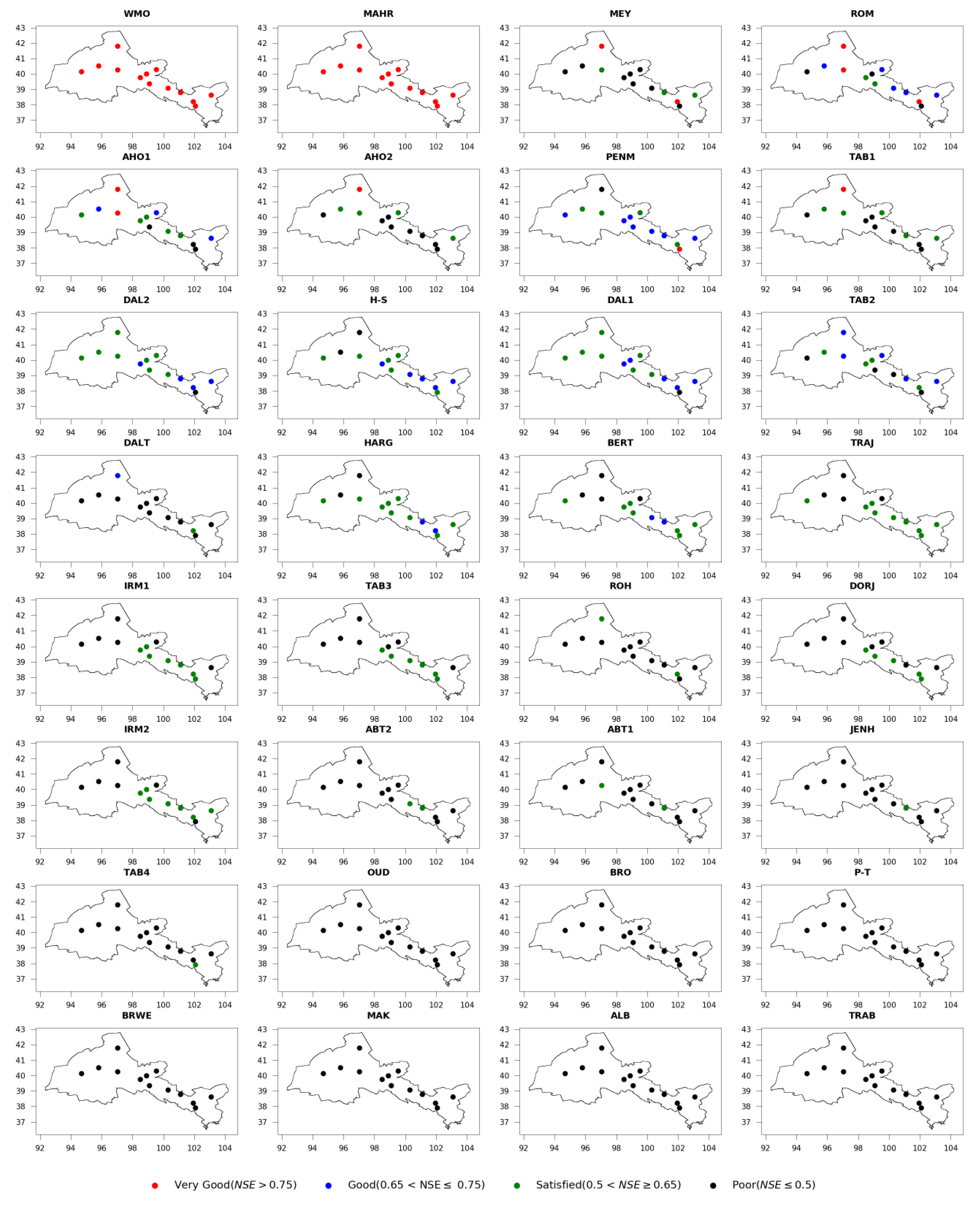
4.2. Cross-Comparison of the ET0 Models

The cross-comparison of the 32 models aimed to distinguish the models with the best performance at each river basin of the Hexi corridor. The mean NSE > 0.75 was taken to be the threshold condition of model selection. From Table S1, the two models (MAHR and WMO) satisfied the conditions of NSE coefficients >0.75 at the daily timescale in all basins (Figure not shown). The MAHR showed better NSE values of 0.91, 0.93, and 0.94 for the Shiyang river basin (SYRB), Shule river basin (SLRB), and Heihe river basin (HRB), respectively. The WMO was also found to estimate the ET0 values with the significant NSE values of 0.97, 0.96, and 0.95 for SYRB, SLRB, and HRB, respectively (Table S1).
A similar condition was applied to the monthly timescale. The results show 13 models that comply with the conditions of NSE coefficients and >0.75. Figure 6 depicts the 13 models selected based on best performance (NSE > 0.75) in the three inland river basins of the Hexi corridor.
The WMO, MAHR, ROM, and DAL1 models ranked as the best methods and showed a very good performance in all three inland river basins. Moreover, DAL1 resulted in low mean PBIAS values of 1.1% and −3.58% for the HRB and SYRB, respectively. The AHO1 model showed the best performance in the SLRB, with the monthly mean NSE and PBIAS of 0.9% and 2.5%, respectively. However, this model is attributed to an overestimation of ET0 with PBIAS averaged to −18.5% and −25.4% in the HRB (Table S1). The H-S, DAL2, HARG, and BERT methods revealed good performance in the SYRB (PBIAS = −0.68%, NSE = 0.77) and the middle reach of the HRB (PBIAS 2.87%, NSE = 0.85). The TAB1, TAB2, and AHO2 are suitable for the SLRB, with monthly mean NSE values of 0.81, 0.83, and 0.82, respectively. The IRM2 performed well in the Heihe river basin only, with NSE = 0.78 and PBIAS = 9.3%. The results analyzed above (Figure 2, Figure 3, Figure 4, Figure 5 and Figure 6) were obtained before the model calibration. However, numerous studies have suggested model calibration to adjust ET0 results to local climate conditions [78,79,80,81].

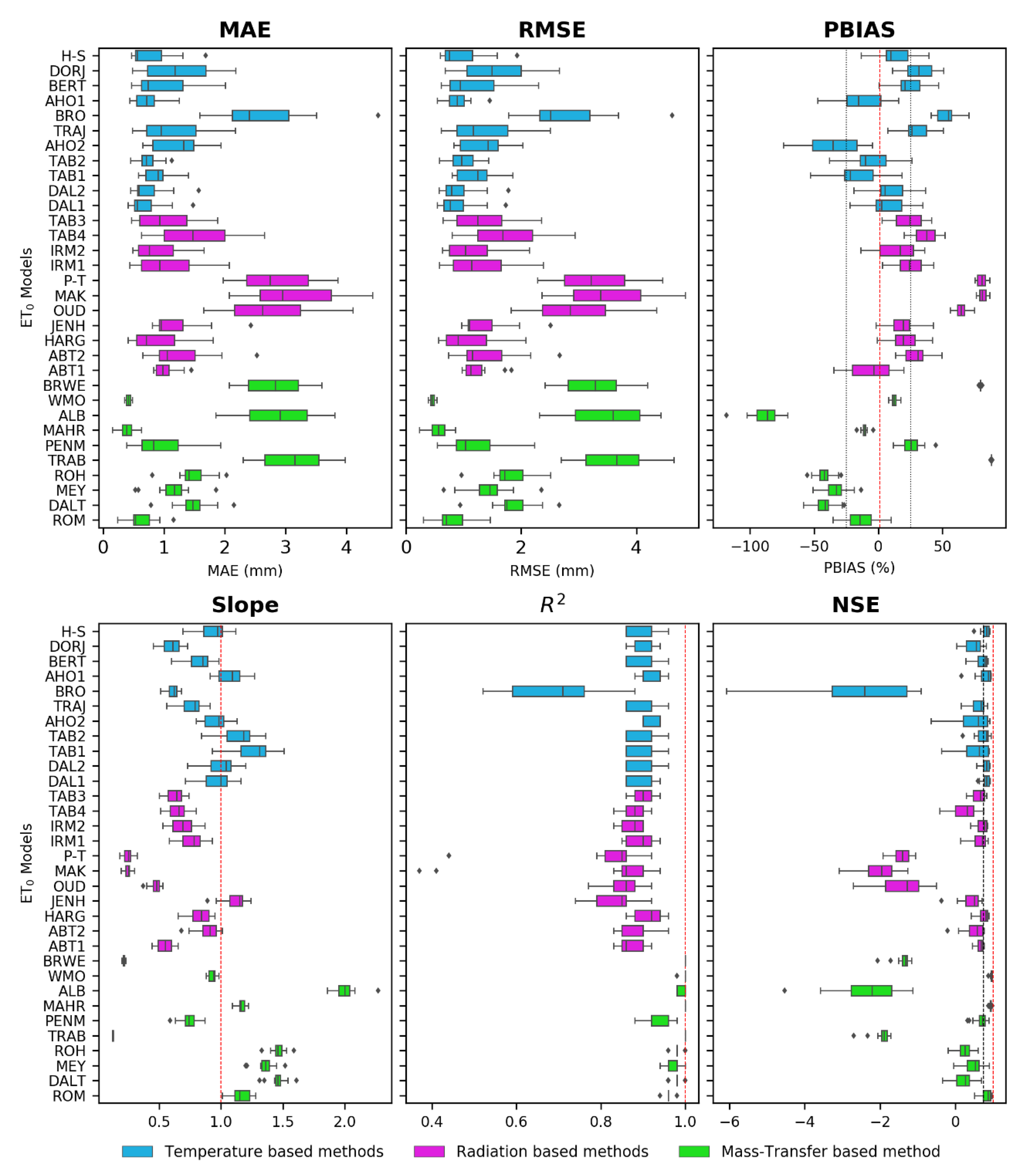
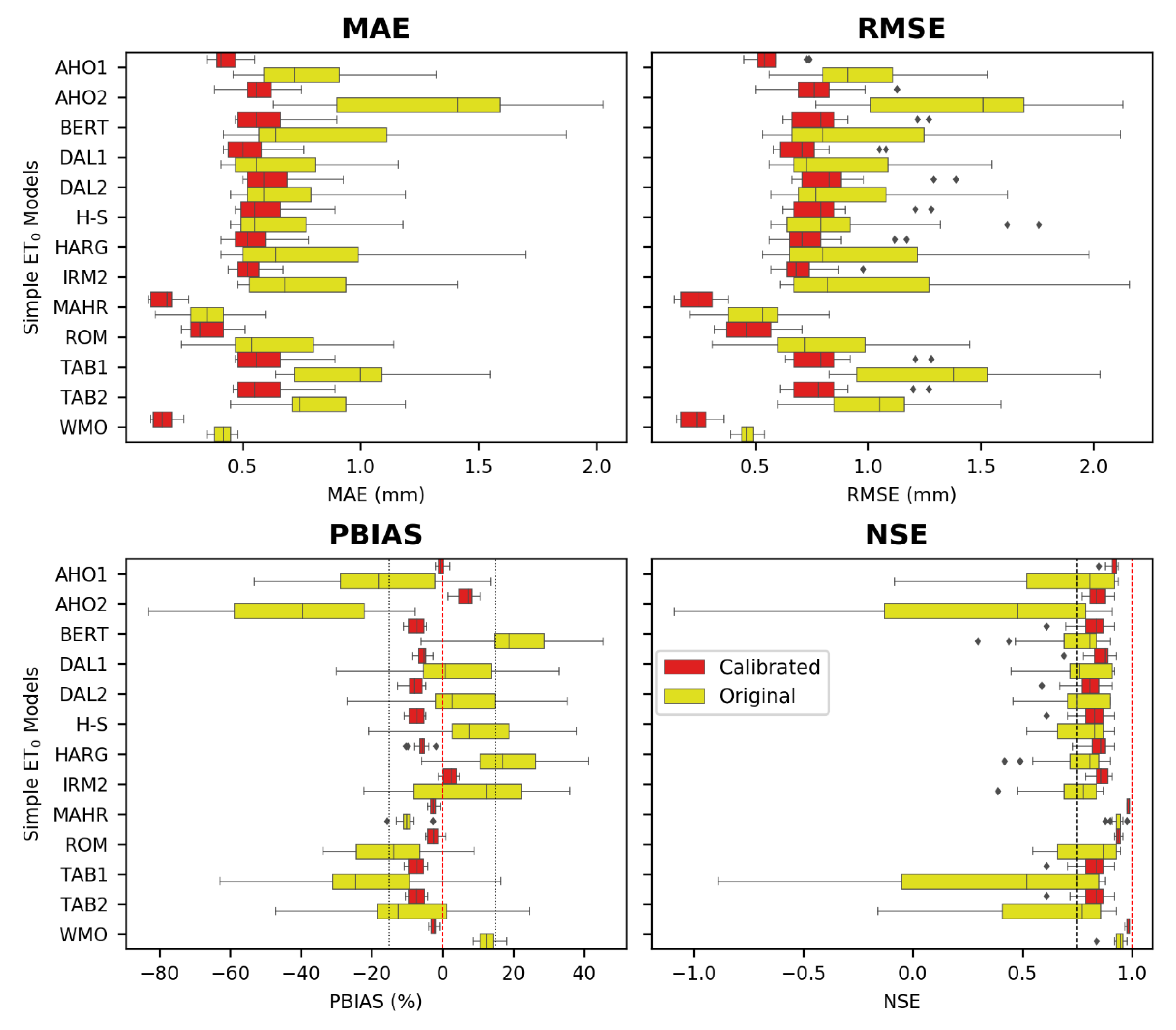
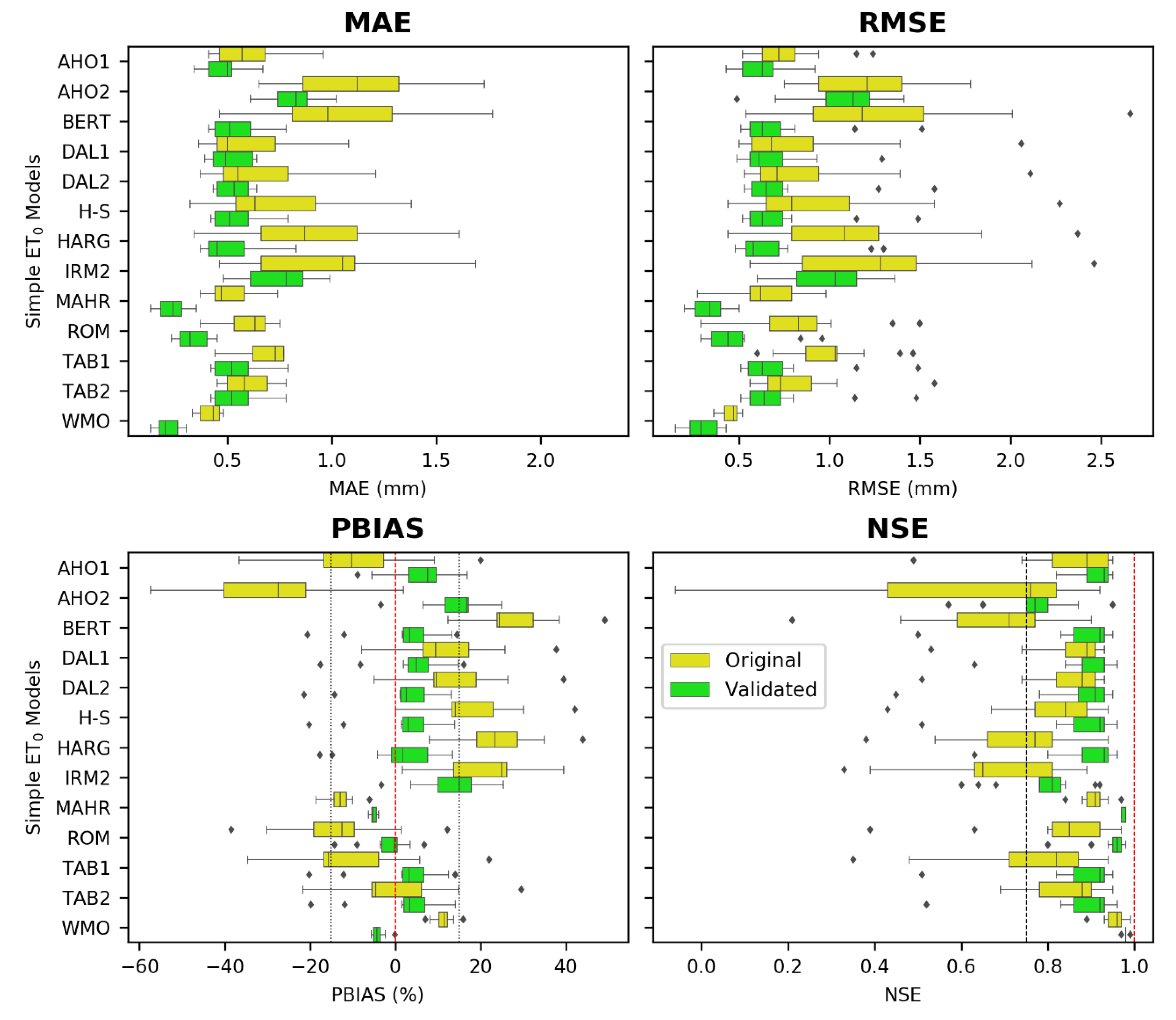
4.3. Calibration of the ET0 Models

In this study, we calibrated models that resulted from the cross-comparison process. The ET0 values from 13 models resulting from cross-comparison were selected to be calibrated. Model results were calibrated against the ET0 estimates from the PM-FAO56 method on a monthly timescale. Figure 7 compares the monthly performances of selected models compared with PM-FAO56 before and after calibration. The regression coefficients used to change the model parameters at each station are shown in Supplementary Table S2.
The calibration process significantly improved the 13 models mentioned above. In fact, it significantly reduced the PBIAS of the ROM method by 82.12% and increased the NSE by 16.7%. The NSE values of the AHO1, IRM2, HARG, and DAL1 methods improved by 33.6%, 19.8%, 13.4%, and 9.3%, respectively, after calibration. The calibration also improved the PBIAS of the AHO2, DAL2, BERT, and H-S methods by 82%, 78.2%, 62.9%, and 18.2%, respectively, after calibration.
An overall improvement in most models was noted in PBIAS values of less than 15% after calibration. The calibration results show that the WMO and MAHR methods remain robust in the Hexi region with the lower mean PBIAS values of −2.5% and −2.6% respectively. The robust performance of the WMO, MAHR, and ROM methods can be explained by the sensitivity of ET0 to the variation of relative humidity in the Hexi corridor [82].
A time series for 2000–2017 was used to validate the calibrated methods. Figure 8 compares the results of the 13 validated methods and PM-FAO56. The results reveal that the WMO, MAHR, and ROM methods remain the best substitute models to estimate the ET0 in the Hexi corridor. They showed robust NSE coefficients of 0.98, 0.98, and 0.95, respectively, and lower MAE and RMSE values than the other validated models. Their RMSE values ranged from 0.15 to 0.43 mm, from 0.20 to 0.50 mm, and from 0.29 to 0.96 mm after validation, respectively.
Comparative studies of different ET0 models against the PM-FAO56 have been documented [73,81,82]. A comparison between the PM-FAO56 method and the 34 ET0 methods showed that the WMO, Droogers, Allen, and Ahooghalandari models performed very well in the semi-arid region of New Mexico [4]. Tabari et al. (2013) found that the Romanenko (ROM) model performed well to estimate ET0 values in the humid climate of Iran [78]. A low performance of the IRM1 method was also reported in Eastern Africa [83]. Peng et al. (2017) evaluated 10 ET0 equations and recommended the Berti method as the best alternative method to estimate monthly ET0 in mainland China [39]. Gao et al. (2017) recommended the Priestley and Taylor model to be the best substitute of the PM-FAO56 in the arid region of Northwest China [32]; however, in the current study, the Priestley and Taylor model did not show a direct promising application in the Hexi corridor.
Previous studies have also shown the best performance of both the Mahringer (MAHR) and WMO models in different regions [77,84,85]. An assessment of 16 ET0 models reported that the MAHR model showed relatively good performance compared to the PM-FAO56 method in the Senegal river basin [84,86]. An overestimation of ET0 values from the MAHR model was observed at some stations of New Mexico, USA [4]. The WMO underestimated ET0 values, which is consistent with the previous results obtained in Malaysia [87].
Shiri (2018) reported poor performance of mass transfer methods in southern Iran, and found that the calibration process improved their performance [74]. The poor performance of the Trabert and Jensen–Haise models in the Hexi corridor is consistent with that reported by Meng Li et al. (2018) in Eastern China [88].
Numerous studies evaluated the Hargreaves and Samani equation and have suggested local calibration to adjust the model to local climate conditions [26,89,90]. Tabari and Talee (2011) showed that the original Hargreaves method underestimated ET0 values, and the calibration of its original empirical coefficient from 0.0023 to 0.0031 improved the model performance in the cold and arid regions of Iran [18].

5. Conclusions

The performance of 32 simple ET0 alternatives, developed based on three approaches (temperature, radiation, and mass transfer-based) to the evapotranspiration produced by the PM-FAO56 method, was assessed for the Hexi Corridor in Northwest China. From our assessment, the World Meteorological Organization (WMO) and Mahringer (MAHR) methods are the most robust. However, the Romanenko (ROM) model is also a good substitute for PM-FAO56, especially in the middle reach of the Heihe river basin and Shiyang river basin. Among the temperature-based methods, the Ahooghalandari (AHO1), Tabari (TAB2) models performed well in the Shule river basin, and the Hargreaves method and its derived equations presented the best performance in the middle reach of the Heihe river basin. A large number of the mass transfer-based methods performed poorly, overestimating ET0 values. The poor performance of the solar radiation-based methods is subjected to an underestimation of ET0 values. Many simple ET0 models tend to perform well on a large timescale basis. Calibration/validation significantly improved all selected models. The results from the calibration procedure of 13 models on a monthly time scale show that the WMO, MAHR, ROM, AHO1, AHO2, DAL1, HARG, IRM2, TRAB, H-S, BERT, TAB1, and DAL2 methods are the best substitute to the PM-FAO56 method for estimating the ET0 in the Hexi corridor.
Moreover, models that integrate temperature, relative humidity, and wind speed (WMO and MAHR) were ranked the best, followed by models that integrate the temperature and relative humidity (ROM, AHO1, and AHO2). The results of this study will be beneficial for selecting the simple ET0 method appropriate for the Hexi corridor and its inland river basins, as well as the local weather stations. When temperature, relative humidity, and wind speed data are available, the WMO method can be used to estimate ET0 values in the Hexi corridor. In the case of missing wind speed and solar radiation, the ROM method can be adopted for estimating ET0 values. The adoption of the DAL1 method is recommended when only temperature data are available.

Supplementary Materials

The following are available online at https://www.mdpi.com/2073-4441/12/10/2772/s1, Table S1: A summary of mean statistical metrics averaged for each river basin before calibration. Table S2: Regression coefficients (Ψ) used to calibrate and validate the 13 ET0 models on a monthly timescale.

Author Contributions

Conceptualization, S.C. and F.Q.; methodology, S.C.; software, S.C. and R.L.; validation, F.Q., R.L., and T.Y.; formal analysis, S.C. and W.C.; resources, F.Q.; data curation, S.C., and F.Q.; writing—original draft preparation, S.C.; writing—review and editing, S.C., R.L., T.Y., W.C. and F.Q.; supervision, F.Q., and R.L.; project administration, F.Q.; funding acquisition, F.Q. All authors have read and agreed to the published version of the manuscript.

Funding

This research was funded by the National Key R&D Program of China (No. 2017YFC0404305), National Natural Science Foundation of China (No. 41801015, No. 41771252) and the Foundation for Excellent Young Scholars of Northwest Institute of Eco-Environment and Resources (NIEER), Chinese Academy of Sciences, CAS (No. 51Y851D61), the Major Program of the Natural Science Foundation of Gansu province, China (No. 18JR4RA002), the Science and Technology Program of Gansu Province, China (18JR2RA026), and the CAS-TWAS President’s Fellowship program.

Conflicts of Interest

The authors declare no conflict of interest.

References

  1. Ndiaye, P.M.; Bodian, A.; Diop, L.; Deme, A.; Dezetter, A.; Djaman, K. Evaluation and Calibration of Alternative Methods for Estimating Reference Evapotranspiration in the Senegal River Basin. Hydrology 2020, 7, 24. [Google Scholar] [CrossRef]
  2. Zhao, L.; Xia, J.; Xu, C.Y.; Wang, Z.; Sobkowiak, L.; Long, C. Evapotranspiration estimation methods in hydrological models. J. Geogr. Sci. 2013, 23, 359–369. [Google Scholar] [CrossRef]
  3. Bandyopadhyay, A.; Bhadra, A.; Swarnakar, R.K.; Raghuwanshi, N.S.; Singh, R. Estimation of reference evapotranspiration using a user-friendly decision support system: DSS_ET. Agric. For. Meteorol. 2012, 154–155, 19–29. [Google Scholar] [CrossRef]
  4. Djaman, K.; O’Neill, M.; Diop, L.; Bodian, A.; Allen, S.; Koudahe, K.; Lombard, K. Evaluation of the penman-monteith and other 34 reference evapotranspiration equations under limited data in a semiarid dry climate. Theor. Appl. Climatol. 2019, 137, 729–743. [Google Scholar] [CrossRef]
  5. Sharma, M.L. Estimating Evapotranspiration. In Advances in Irrigation; Hillel, D., Ed.; Academic Press: New York, NY, USA, 1985; pp. 213–281. ISBN 0275-7915. [Google Scholar]
  6. Berti, A.; Tardivo, G.; Chiaudani, A.; Rech, F.; Borin, M. Assessing reference evapotranspiration by the Hargreaves method in North-Eastern Italy. Agric. Water Manag. 2014, 140, 20–25. [Google Scholar] [CrossRef]
  7. Ahooghalandari, M.; Khiadani, M.; Jahromi, M.E. Developing equations for estimating reference evapotranspiration in Australia. Water Resour. Manag. 2016, 30, 3815–3828. [Google Scholar] [CrossRef] [Green Version]
  8. Ahooghalandari, M.; Khiadani, M.; Jahromi, M.E. Calibration of Valiantzas’ reference evapotranspiration equations for the Pilbara region, Western Australia. Theor. Appl. Climatol. 2017, 128, 845–856. [Google Scholar] [CrossRef]
  9. Quej, V.H.; Martí, P. Global performance ranking of temperature-based approaches for evapotranspiration estimation considering Köppen climate classes. J. Hydrol. 2015, 528, 514–522. [Google Scholar] [CrossRef]
  10. Priestley, C.H.B.; Taylor, R.J. On the assessment of surface heat flux and evaporation using large-scale parameters. Mon. Weather Rev. 1972, 100, 81–92. [Google Scholar] [CrossRef]
  11. Trajkovic, S. Temperature-based approaches for estimating reference evapotranspiration. J. Irrig. Drain Eng. 2005, 131, 316–323. [Google Scholar] [CrossRef]
  12. Allen, R.G.; Pereira, L.S.; Raes, D.; Smith, M. Crop evapotranspiration: Guidelines for computing crop water requirements. FAO Irrig. Drain. Pap. 1998, 56, 300. [Google Scholar]
  13. Allen, R.G.; Clemmens, A.J.; Burt, C.M.; Solomon, K.; O’Halloran, T. Prediction accuracy for projectwide evapotranspiration using crop coefficients and reference evapotranspiration. J. Irrig. Drain Eng. 2005, 131, 24–36. [Google Scholar] [CrossRef] [Green Version]
  14. Allen, R.G.; Pruitt, W.O.; Wright, J.L.; Howell, T.A.; Ventura, F.; Snyder, R.; Itenfisu, D.; Steduto, P.; Berengena, J.; Yrisarry, J.B.; et al. A recommendation on standardized surface resistance for hourly calculation of reference ETo by the FAO56 penman-monteith method. Agric. Water Manag. 2006, 81, 1–22. [Google Scholar] [CrossRef]
  15. Sahli, A. Evaluation of FAO-56 methodology for estimating reference evapotranspiration using limited climatic data application to Tunisia. Agric. Water Manag. 2008, 95, 707–715. [Google Scholar] [CrossRef]
  16. Berengena, J.; Allen, R.G. Measuring versus estimating net radiation and soil heat flux: Impact on penman–monteith reference ET estimates in semiarid regions. Agric. Water Manag. 2007, 89, 275–286. [Google Scholar] [CrossRef]
  17. Pizza, S.; Caponio, T.; Rivelli, A.R.; Perniola, M. Lysimetric determination of muskmelon crop coefficients cultivated under plastic mulches. Agric. Water Manag. 2005, 72, 147–159. [Google Scholar] [CrossRef]
  18. Tabari, H.; Talaee, P.H. Local calibration of the hargreaves and priestley-taylor equations for estimating reference evapotranspiration in arid and cold climates of iran based on the penman-monteith model. J. Hydrol. Eng. 2011, 16, 837–845. [Google Scholar] [CrossRef]
  19. Dorji, U.; Olesen, J.E.; Seidenkrantz, M.S. Water balance in the complex mountainous terrain of Bhutan and linkages to land use. J. Hydrol. Reg. Stud. 2016, 7, 55–68. [Google Scholar] [CrossRef] [Green Version]
  20. Droogers, P.; Allen, R.G. Estimating reference evapotranspiration under inaccurate data conditions. Irrig. Drain. Syst. 2002, 16, 33–45. [Google Scholar] [CrossRef]
  21. Trajkovic, S. Hargreaves versus penman-monteith under humid conditions. J. Irrig. Drain. Eng. 2007, 133, 38–42. [Google Scholar] [CrossRef]
  22. Hargreaves, G.; Allen, R. History and evaluation of hargreaves evapotranspiration equation. J. Irrig. Drain. Eng. 2003, 129, 53–63. [Google Scholar] [CrossRef]
  23. Heydari, M.M.; Heydari, M. Calibration of hargreaves–Samani equation for estimating reference evapotranspiration in semiarid and arid regions. Arch. Fèur Acker Pflanzenbau Bodenkd. 2014, 60, 695–713. [Google Scholar] [CrossRef]
  24. Gafurov, Z.; Eltazarov, S.; Akramov, B.; Yuldashev, T.; Djumaboev, K.; Anarbekov, O. Modifying hargreaves-samani equation for estimating reference evapotranspiration in dryland regions of Amudarya River Basin. Agric. Sci. 2018, 9, 1354–1368. [Google Scholar] [CrossRef] [Green Version]
  25. Amatya, D.M.; Skaggs, R.W.; Gregory, J.D. Comparison of methods for estimating REF-ET. J. Irrig. Drain. Eng. 1995, 121, 427–435. [Google Scholar] [CrossRef]
  26. Feng, Y.; Jia, Y.; Cui, N.; Zhao, L.; Li, C.; Gong, D. Calibration of Hargreaves model for reference evapotranspiration estimation in Sichuan basin of southwest China. Agric. Water Manag. 2017, 181, 1–9. [Google Scholar] [CrossRef]
  27. Lima, J.R.D.S.; Antonino, A.C.D.; Souza, E.S.D.; Hammecker, C.; Montenegro, S.M.G.L.; Lira, C.A.B.D.O. Calibration of hargreaves-samani equation for estimating reference evapotranspiration in Sub-Humid region of Brazil. J. Water Reour. Prot. 2013, 5, 1–5. [Google Scholar] [CrossRef] [Green Version]
  28. Mehdizadeh, S.; Saadatnejadgharahassanlou, H.; Behmanesh, J. Calibration of hargreaves–samani and priestley–taylor equations in estimating reference evapotranspiration in the Northwest of Iran. Arch. Fèur Acker Pflanzenbau Bodenkd. 2017, 63, 942–955. [Google Scholar] [CrossRef]
  29. Pereira, L.S. Estimation of ETo with hargreaves–samani and FAO-PM temperature methods for a wide range of climates in Iran. Agric. Water Manag. 2013, 121, 1–18. [Google Scholar] [CrossRef]
  30. Rahimi Khoob, A. Comparative study of Hargreaves’s and artificial neural network’s methodologies in estimating reference evapotranspiration in a semiarid environment. Irrig. Sci. 2008, 26, 253–259. [Google Scholar] [CrossRef]
  31. Gao, F.; Feng, G.; Ouyang, Y.; Wang, H.; Fisher, D.; Adeli, A.; Jenkins, J. Evaluation of Reference Evapotranspiration Methods in Arid, Semiarid, and Humid Regions. J. Am. Water Resour. Assoc. 2017, 53, 791–808. [Google Scholar] [CrossRef]
  32. Ahmed, H.I.; Liu, J. Evaluating reference crop evapotranspiration (ETo) in the centre of guanzhong basin—Case of Xingping & Wugong, Shaanxi, China. Engineering 2013, 5, 459–468. [Google Scholar] [CrossRef] [Green Version]
  33. Wenhuan, B.; Yawei, L.; Haiyu, W.; Shihong, Y.; Zheng, W. Modeling rice development and field water balance using AquaCrop model under drying-wetting cycle condition in eastern China. Agric. Water Manag. 2019, 213, 289–297. [Google Scholar] [CrossRef]
  34. Bourque, C.P.A. Assessing spatiotemporal variation in actual evapotranspiration for semi-arid watersheds in northwest China: Evaluation of two complementary-based methods. J. Hydrol. 2013, 486, 455–465. [Google Scholar] [CrossRef]
  35. Cui, N.; Zhao, L.; Hu, X.; Gong, D. Comparison of ELM, GANN, WNN and empirical models for estimating reference evapotranspiration in humid region of Southwest China. J. Hydrol. 2016, 536, 376–383. [Google Scholar] [CrossRef]
  36. Erda, L. Performance of the priestley–Taylor equation in the semiarid climate of North China. Agric. Water Manag. 2005, 71, 1–17. [Google Scholar] [CrossRef]
  37. Gao, X.; Peng, S.; Xu, J.; Shihong, Y.; Wang, W. Proper methods and its calibration for estimating reference evapotranspiration using limited climatic data in Southwestern China. Arch. Fèur Acker Pflanzenbau Bodenkd. 2015, 61, 415–426. [Google Scholar] [CrossRef]
  38. Luo, Y.; Conglin, W.; Hezhen, Z.; Lei, Z.; Yuanlai, C.; Ningning, S.; Wang, L. Evaluation of six equations for daily reference evapotranspiration estimating using public weather forecast message for different climate regions across China. Agric. Water Manag. 2019, 222, 386–399. [Google Scholar] [CrossRef]
  39. Peng, L.; Li, Y.; Feng, H. The best alternative for estimating reference crop evapotranspiration in different sub-regions of mainland China. Sci. Rep. 2017, 7, 5458. [Google Scholar] [CrossRef] [Green Version]
  40. Song, X.; Lu, F.; Xiao, W.; Zhu, K.; Zhou, Y.; Xie, Z. Performance of 12 reference evapotranspiration estimation methods compared with the penman-monteith method and the potential influences in northeast China. Meteorol. Appl. 2019, 26, 83–96. [Google Scholar] [CrossRef] [Green Version]
  41. Wu, S.; Zheng, D.; Yang, Q. Radiation calibration of FAO56 penman–Monteith model to estimate reference crop evapotranspiration in China. Agric. Water Manag. 2008, 95, 77–84. [Google Scholar] [CrossRef]
  42. Valiantzas, J.D. Simplified limited data penman’s ET0 formulas adapted for humid locations. J. Hydrol. 2015, 524, 701–707. [Google Scholar] [CrossRef]
  43. Romanenko, V.A. Computation of the autumn soil moisture using a universal relationship for a large area. Proc. Ukr. Hydrometeorol. Res. Inst. 1961, 3, 12–25. [Google Scholar]
  44. Makkink, G.F. Testing the penman formula by means of lysimeters. J. Inst. Water Eng. 1957, 11, 277–288. [Google Scholar]
  45. Turk, L. Estimation of irrigation water requirements, potential evapotranspiration: A simple climatic formula evolved up to date. Ann. Agron. 1961, 12, 13–14. [Google Scholar]
  46. Valiantzas, J.D. Simplified versions for the penman evaporation equation using routine weather data. J. Hydrol. 2006, 331, 690–702. [Google Scholar] [CrossRef]
  47. Deng, Y.; Gou, X.; Gao, L.; Yang, M.; Zhang, F. Tree-ring recorded moisture variations over the past millennium in the Hexi Corridor, northwest China. Environ. Earth Sci. 2017, 76, 272. [Google Scholar] [CrossRef]
  48. Fang, C.L. Water resources constraint force on urbanization in water deficient regions: A case study of the Hexi Corridor, arid area of NW China. Ecol. Econ. 2007, 62, 508–517. [Google Scholar] [CrossRef]
  49. Tong, L.; Niu, J.; Kang, S.; Du, T.; Li, S.; Ding, R. Spatio-temporal distribution of irrigation water productivity and its driving factors for cereal crops in Hexi Corridor, Northwest China. Agric. Water Manag. 2017, 179, 55–63. [Google Scholar] [CrossRef]
  50. Wu, G.; Pan, B.; Guan, Q.; Liu, Z.; Li, J. Loess record of climatic changes during MIS5 in the Hexi Corridor, northwest China. Quat. Int. 2002, 97–98, 167–172. [Google Scholar] [CrossRef]
  51. Dodson, J.R.; Li, X.; Zhou, X.; Zhao, K.; Sun, N.; Atahan, P. Origin and spread of wheat in China. Quat. Sci. Rev. 2013, 72, 108–111. [Google Scholar] [CrossRef]
  52. Fu, J.; Niu, J.; Kang, S.; Adeloye, A.J.; Du, T. Crop production in the hexi corridor challenged by future climate change. J. Hydrol. 2019, 579. [Google Scholar] [CrossRef]
  53. Li, X.; Zhang, X.; Niu, J.; Tong, L.; Kang, S.; Du, T.; Li, S.; Ding, R. Irrigation water productivity is more influenced by agronomic practice factors than by climatic factors in Hexi Corridor, Northwest China. Sci. Rep. 2016, 6, 37971. [Google Scholar] [CrossRef] [PubMed]
  54. Hargreaves, H.G.; Samani, A.Z. Reference crop evapotranspiration from temperature. Appl. Eng. Agric. 1985, 1, 96–99. [Google Scholar] [CrossRef]
  55. Jensen, M.E.; Haise, H.R. Estimating evapotranspiration from solar radiation. Proc. Am. Soc. Civil Eng. 1963, 89, 15–41. [Google Scholar]
  56. Caprio, J. The Solar Thermal Unit Concept in Problems Related to Plant Development and Potential Evapotranspiration. In Phenology and Seasonality Modeling. Ecological Studies (Analysis and Synthesis); Lieth, H., Ed.; Springer: Berlin/Heidelberg, Germany; New York, NY, USA, 1974; ISBN 978-3-642-51865-2. [Google Scholar]
  57. George, H. Hargreaves. Moisture availability and crop production. Trans. ASABE 1975, 18, 980–984. [Google Scholar] [CrossRef]
  58. Abtew, W. Evapotranspiration measurements and modeling for three wetland systems in south Florida. J. Am. Water Resour. Assoc. 1996, 32, 465–473. [Google Scholar] [CrossRef]
  59. Irmak, S.A.; Allen, R.; Jones, A.J. Solar and net radiation-based equations to estimate reference evapotranspiration in humid climates. J. Irrig. Drain. Eng. 2003, 129, 336–347. [Google Scholar] [CrossRef]
  60. Rohwer, C. Evaporation from Free Water Surface; United States Department of Agriculture: Washington, DC, USA, 1931. [Google Scholar]
  61. Mahringer, W. Verdunstungsstudien am Neusiedler See. Theor. Appl. Climatol. 1970, 18, 1–20. [Google Scholar] [CrossRef]
  62. Dalton, J. Experimental essays on the constitution of mixed gases: On the force of steam or vapour from water and other liquids in different temperatures, both in a Torricellian vacuum and in air: On evaporation and on the expansion of gases. Mem. Lit. Philos. Soc. Manch. 1802, 5, 535–602. [Google Scholar]
  63. Xiang, K.; Li, Y.; Horton, R.; Feng, H. Similarity and difference of potential evapotranspiration and reference crop evapotranspiration—A review. Agric. Water Manag. 2020, 232, 106043. [Google Scholar] [CrossRef]
  64. Singh, V.P.; Xu, C.Y. Evaluation and Generalization of 13 equations for determining free water evaporation. Hydrol. Process. 1997, 11, 311–323. [Google Scholar] [CrossRef]
  65. Baier, W.; Robertson, G.W. Estimation of latent evaporation from simple weather observations. Can. J. Plant Sci. 1965, 45, 276–284. [Google Scholar] [CrossRef]
  66. Meyer, A. Ueber Einige Zusammenhänge Zwischen Klima und Boden in Europa; ETH: Zurich, Switzerland, 1926. [Google Scholar]
  67. Albrecht, F. Die methoden zur bestimmung der verdunstung der natürlichen erdoberfläche. Theor. Appl. Climatol. 1950, 2, 1–38. [Google Scholar] [CrossRef]
  68. WMO. Measurement and Estimation of Evaporation and Evapotranspiration. Technical Note No.83; Report of a Working Group on Evaporation Measurement of the Commission for Instrument and Methods of Observation; WMO: Geneva, Switzerland, 1966. [Google Scholar]
  69. Trabert, W. Neue beobachtungen über verdampfungsgeschwindigkeiten. Meteorol. Z. 1896, 13, 261–263. [Google Scholar]
  70. Brockamp, B.; Wenner, H. Verdunstungsmessungen auf den Steiner See bei Mu¨nster. Dt Gewässerkl. Mitt 1963, 7, 149–154. [Google Scholar]
  71. Penman, H.L. Vegetation and hydrology. Commonwealth bureau of soils, harpenden. Technical Communication No. 53; Commonwealth agricultural bureaux. Q.J.R. Meteorol. Soc. 1963, 89, 565–566. [Google Scholar] [CrossRef]
  72. Bos, M.G. Water Requirements for Irrigation and the Environment; Springer: Dordrecht, The Netherlands, 2009; ISBN 1402089481. [Google Scholar]
  73. Moriasi, D.N.; Arnold, J.G.; van Liew, W.M.; Bingner, R.L.; Harmel, R.D.; Veith, T.L. Model evaluation guidelines for systematic quantification of accuracy in watershed simulations. Trans. ASABE 2007, 50, 885–900. [Google Scholar] [CrossRef]
  74. Shiri, J. Improving the performance of the mass transfer-based reference evapotranspiration estimation approaches through a coupled wavelet-random forest methodology. J. Hydrol. 2018, 561, 737–750. [Google Scholar] [CrossRef]
  75. Shiri, J. Evaluation of FAO56-PM, empirical, semi-empirical and gene expression programming approaches for estimating daily reference evapotranspiration in hyper-arid regions of Iran. Agric. Water Manag. 2017, 188, 101–114. [Google Scholar] [CrossRef]
  76. Shiri, J.; Sadraddini, A.A.; Nazemi, A.H.; Marti, P.; Fakheri Fard, A.; Kisi, O.; Landeras, G. Independent testing for assessing the calibration of the Hargreaves–Samani equation New heuristic alternatives for Iran. Comput. Electron. Agric. 2015, 117, 70–80. [Google Scholar] [CrossRef]
  77. Valipour, M. Calibration of mass transfer-based models to predict reference crop evapotranspiration. Appl. Water Sci. 2017, 7, 625–635. [Google Scholar] [CrossRef] [Green Version]
  78. Didari, S.; Ahmadi, S.H. Calibration and evaluation of the FAO56-Penman-Monteith, FAO24-radiation, and Priestly-Taylor reference evapotranspiration models using the spatially measured solar radiation across a large arid and semi-arid area in southern Iran. Theor. Appl. Climatol. 2019, 136, 441–455. [Google Scholar] [CrossRef]
  79. Valiantzas, J.D. Temperature-and humidity-based simplified Penman’s ET0 formulae. Comparisons with temperature-based hargreaves-samani and other methodologies. Agric. Water Manag. 2018, 208, 326–334. [Google Scholar] [CrossRef]
  80. Xu, J.; Peng, S.; Ding, J.; Wei, Q.; Yu, Y. Evaluation and calibration of simple methods for daily reference evapotranspiration estimation in humid East China. Arc. Fèur Acker Pflanzenbau Bodenkd. 2013, 59, 845–858. [Google Scholar] [CrossRef]
  81. Maneta, M.P.; Schnabel, S.; Wallender, W.W.; Panday, S.; Jetten, V. Calibration of an evapotranspiration model to simulate soil water dynamics in a semiarid rangeland. Hydrol. Process. 2008, 22, 4655–4669. [Google Scholar] [CrossRef]
  82. Xu, Z.W.; Zuo, D.P.; Wang, X.M. Temporal variations of reference evapotranspiration and its sensitivity to meteorological factors in Heihe River Basin, China. Water Sci. Eng. 2015, 8, 1–8. [Google Scholar] [CrossRef] [Green Version]
  83. Djaman, K.; Irmak, S.; Futakuchi, K. Daily Reference evapotranspiration estimation under limited data in Eastern Africa. J. Irrig. Drain. Eng. 2017, 143, 6016015. [Google Scholar] [CrossRef]
  84. Balde, A.B.; Sow, A.; Muller, B.; Irmak, S.; N’Diaye, M.K.; Baboucarr, M.; Moukoumbi, Y.D.; Futakuchi, K.; Saito, K. Evaluation of sixteen reference evapotranspiration methods under sahelian conditions in the Senegal River Valley. J. Hydrol. Reg. Stud. 2015, 3, 139–159. [Google Scholar] [CrossRef] [Green Version]
  85. Valipour, M. Application of new mass transfer formulae for computation of evapotranspiration. J. Appl. Water Eng. Res. 2014, 2, 33–46. [Google Scholar] [CrossRef]
  86. Djaman, K.; Tabari, H.; Balde Alpha, B.; Diop, L.; Futakuchi, K.; Irmak, S. Analyses, calibration and validation of evapotranspiration models to predict grass-reference evapotranspiration in the Senegal river delta. J. Hydrol. Reg. Stud. 2016, 8, 82–94. [Google Scholar] [CrossRef] [Green Version]
  87. Muhammad, M.; Nashwan, M.; Shahid, S.; Ismail, T.; Song, Y.; Chung, E.S. Evaluation of empirical reference evapotranspiration models using compromise programming: A case study of Peninsular Malaysia. Sustainability 2019, 11, 4267. [Google Scholar] [CrossRef] [Green Version]
  88. Li, M.; Chu, R.; Islam, A.R.M.T.; Shen, S. Reference evapotranspiration variation analysis and its approaches evaluation of 13 empirical models in sub-humid and humid regions a case study of the Huai River Basin, Eastern China. Water 2018, 10, 493. [Google Scholar] [CrossRef] [Green Version]
  89. Rahimikhoob, A.; Behbahani, M.R.; Fakheri, J. An evaluation of four reference evapotranspiration models in a subtropical climate. Water Resour. Manag. 2012, 26, 2867–2881. [Google Scholar] [CrossRef]
  90. Almorox, J.; Grieser, J. Calibration of the Hargreaves–Samani method for the calculation of reference evapotranspiration in different Köppen climate classes. Hydrol. Res. 2016, 47, 521–531. [Google Scholar] [CrossRef] [Green Version]
Figure 1. Digital elevation model (DEM) of Hexi Corridor, and distribution of meteorological stations in three inland river basins namely Shule river basin (SLRB), Heihe river basin (HRB), and Shiyang river basin (SYRB).
Water 12 02772 g001
Figure 2. Daily performance of the simple ET0 methods according to the selected evaluation metrics herein mean absolute errors (MAE), root mean square errors (RMSE), percentage bias (PBIAS), regression slope (Slope), coefficient of determination (R2), and Nash–Sutcliffe efficient (NSE). The red and black dash lines depict the optimum and threshold values of an evaluated metric, respectively.
Water 12 02772 g002
Figure 3. Performance of 32 ET0 methods according to the selected evaluation metrics on monthly data in the Hexi Corridor, (a) mean absolute errors (MAE), (b) root mean square errors (RMSE), (c) percentage bias (PBIAS), (d) regression slope(Slope), (e) coefficient of determination (R2), and (f) Nash–Sutcliffe efficient (NSE).
Water 12 02772 g003
Figure 4. Spatial distribution of daily Nash–Sutcliffe efficient (NSE) values computed from the 32 simple ET0 models in reference of the PM-FAO56 method over the Hexi corridor region (Full names of each model are shown in Table 2).
Water 12 02772 g004
Figure 5. Spatial distribution of monthly Nash–Sutcliffe efficient (NSE) values computed from the 32 simple ET0 models in reference of the PM-FAO56 method over the Hexi corridor region (Full names of each model are shown in Table 2).
Water 12 02772 g005
Figure 6. Cross-comparison between 13 robust methods (dash line represents the threshold value for model selection condition, NSE = 0.75).
Water 12 02772 g006
Figure 7. Model performance before (original) and after calibration (calibrated) on a monthly timescale over the period 1960–1999. The models are assessed through the MAE, RMSE, PBIAS and NSE.
Water 12 02772 g007
Figure 8. Performance of the 13 validated models on a monthly timescale over the period 2000–2017. The models are assessed through the MAE, RMSE, PBIAS and NSE metrics respectively.
Water 12 02772 g008
Table 1. Properties of thirteen meteorological stations with long-term average climatic conditions. minimum, mean, and maximum air temperature (Tmin, Tmean, and Tmax), mean, maximum, and minimum relative humidity (Rhmean, Rhmax and RHmin), wind speed measured at 10 m height (U10m), sunshine duration (SSD), and solar radiation (Rs).
BasinStationLatitude
°N
Longitude
°E
Elevation
M
Tmean
°C
Tmax
°C
Tmin
°C
Rhmean
%
RHmax
%
RHmin
%
U10m
m/s
SSD
h
Rs
MJ/m2
SLRBMazongshan41.897.0317704.5312.3−2.439.459.6719.14.479.1717.36
Dunhuang40.294.6811399.7918.182.1642.263.5320.42.028.9417.51
Guazhou40.595.7811719.0917.621.8240.359.5221.53.038.7117.13
Yumenzhen40.397.0315267.2814.790.4742.261.7322.43.598.8317.3
HRBDingxin40.399.5211778.5316.651.3643 67.0121.43.079.1217.62
Jinta4098.8812718.5616.461.344465.6922.42.528.9617.49
Jiuquan39.898.4814777.6115.021.194768.3225.32.238.4216.89
Gaotai39.499.0813327.9916.141.1552.879.8525.42.058.4917.06
Zhangye39.1100.314617.5715.950.651.277.0224.72.138.4517.08
Shangdan38.8101.117666.7114.830.0446.968.4323.92.377.9816.53
SYRBYongchang38.2101.920945.2712.75−1.051.675.0127.52.938.1316.76
Wuwei37.9102.115328.3715.651.9651.173.9526.31.767.9516.64
Minqin38.6103.113688.5616.261.6644.365.5322.12.648.4917.19
Table 2. Formulation and data requirement of the ET0 models used in this study.
NoAuthors/ModelsAbbreviationMethods/FormulationLatitudeElevationTmeanTmaxTminRHmeanRHmaxRHminU2mRs
Combination-based methods
(1)Penman–Monteith [12]FAO56 E T 0 = 0.408 Δ ( R n G ) + γ [ 900 / ( T m e a n + 273 ) ] u 2 ( e s e a ) Δ + γ ( 1 + 0.34 u 2 )
Temperature-based methods
(2)Hargreaves and
Samani (1985) [54]
H-S E T 0 = [ 0.0023 × R a ( T m e a n + 17.8 ) ( T max T min ) 0.5 ] / λ
(3)Trajkovic (2007) [21]TRAJ E T 0 = [ 0.0023 × R a ( T m e a n + 17.8 ) ( T max T min ) 0.424 ] / λ
(4)Tabari and
Talaee-1 (2011) [18]
TAB1 E T 0 = [ 0.0031 × R a ( T m e a n + 17.8 ) ( T max T min ) 0.5 ] / λ
(5)Tabari and
Talaee-2 (2011) [18]
TAB2 E T 0 = [ 0.0028 × R a ( T m e a n + 17.8 ) ( T max T min ) 0.5 / λ ]
(6)Droogers and
Allen-1 (2002) [20]
DAL1 E T 0 = [ 0.003 × R a ( T m e a n + 20 ) ( T max T min ) 0.4 ] / λ
(7)Droogers and
Allen-2 (2002) [20]
DAL2 E T 0 = [ 0.0025 × R a ( T m e a n + 16.8 ) ( T max T min ) 0.5 ] / λ
(8)Berti et al. (2014) [6]BERT E T 0 = [ 0.00193 × R a ( T m e a n + 17.8 ) ( T max T min ) 0.517 ] / λ
(9)Dorji et al. (2016) [19]DORJ E T 0 = [ 0.002 × R a ( T m e a n + 33.9 ) ( T max T min ) 0.296 ] / λ
(10)Baier and
Robertson (1965) [65]
BRO E T 0 = 0.109 × ( R a / λ ) + 0.157 T max + 0.158 ( T max T min ) 5.39
(11)Ahooghalandari-1 (2016) [7]AHO1 E T 0 = 0.252 ( R a / λ ) + 0.221 T m e a n ( 1 R H m e a n / 100 )
(12)Ahooghalaandari-2 (2016) [7]AHO2 E T 0 = 0.29 ( R a / λ ) + 0.15 T max ( 1 R H m e a n / 100 )
Solar radiation- based methods
(13)Makkink (1957) [44]MAK E T 0 = 0.7 × ( R s / λ ) × [ Δ / Δ + γ ] 0.12
(14)Priestley and Tayler (1972) [10]P-T E T 0 = 1.26 ( R n G ) [ Δ / Δ + γ ] / λ
(15)Jensen and Haise(1963) [55]JENH E T 0 = ( 0.025 T m e a n + 0.08 ) R s / λ
(16)Hargreaves (1975) [57]HARG E T 0 = [ 0.0135 ( T m e a n + 17.8 ) R s ] / λ
(17)Abtew-1(1996) [58]ABT1 E T 0 = 0.52 T max R s / λ
(18)Abtew-2(1996) [58]ABT2 E T 0 = ( T max / 56 ) × ( R s / λ )
(19)Irmak et al. (2003)-1 [59]IRM1 E T 0 = 0.611 + 0.149 R s + 0.079 T m e a n
(20)Irmak et al. (2003)-2 [59]IRM2 E T 0 = 0.469 + 0.289 R n + 0.023 T m e a n
(21)Tabari and Talaee (2011) [18]TAB3 E T 0 = 0.642 + 0.174 R s + 0.0353 T m e a n
(22)Tabari and Talaee (2011) [18]TAB4 E T 0 = 0.478 + 0.156 R s 0.0112 T max + 0.0733 T min
(23)Oudin (2004) [65]OUD E T 0 = ( R s / λ ) × [ T m e a n + 5 ] / 100
Mass transfer-based methods
(24)Dalton (1802) [63]DALT E T 0 = ( 3.648 + 0.7223 u 2 ) ( e s e a )
(25)Meyer (1926) [66] MEY E T 0 = ( 3.75 + 0.503 u 2 ) ( e s e a )
(26)Rohwer (1931) [60]ROH E T 0 = ( 3.3 + 0.891 u 2 ) ( e s e a )
(27)Albrecht (1950) [67]ALB E T 0 = ( 1.005 + 2.97 u 2 ) ( e s e a )
(28)WMO (1966) [68]WMO E T 0 = ( 1.298 + 0.934 u 2 ) ( e s e a )
(29)Trabert (1896) [69]TRAB E T 0 = 0.3075 × u 2 0.5 ( e s e a )
(30)Brockamp and Wenner (1963) [70]BRWE E T 0 = 0.543 × u 2 0.456 ( e s e a )
(31)Mahringer (1970) [61]MAHR E T 0 = 0.286 × u 2 0.5 ( e s e a )
(32)Penman (1948) [71]PENM E T 0 = ( 2.625 + 0.000479 u 2 ) ( e s e a )
(33)Romanenko (1961) [43]ROM E T 0 = 0.00006 ( 100 R H m e a n ) ( 25 + T m e a n ) 2
ET0: reference crop evapotranspiration (mm day−1); ea: actual vapor pressure (kPa); es: saturation vapor pressure (kPa); (es − ea): saturation vapor pressure deficit (kPa); G: soil heat flux density (mm day−1); n: actual duration of sunshine in a day (h); Ra: extraterrestrial radiation (mm day−1); RHmean: mean relative humidity (%); RHmax: maximum relative humidity (%); RHmin: minimum relative humidity (%); Rn: net solar radiation (MJ/m2 day); Rs: solar radiation (MJ m−2 day−1); Tmean: mean daily temperature (°C); u2: wind speed measured at 2 m height (m s−1); Δ: slope of saturation vapor pressure curve (mb °C−1); γ: psychrometric constant, (kPa °C−1); λ: latent heat of vaporization (MJ kg−1).
Publisher’s Note: MDPI stays neutral with regard to jurisdictional claims in published maps and institutional affiliations.

