Article

Contribution of Phoretic and Electrostatic Effects to the Collection Efficiency of Submicron Aerosol Particles by Raindrops

1
Institut de Radioprotection et de Sûreté Nucléaire (IRSN), PSN-RES, SCA, LPMA, 91192 Gif-sur-Yvette, France
2
Institut de Radioprotection et de Sûreté Nucléaire (IRSN), PSE-SANTE, SESUC, BMCA, 92210 Fontenay-aux-Roses, France
3
Laboratoire de Météorologie Physique, CNRS UMR6016, Université Clermont Auvergne, 63178 Aubière, France
4
CNRS UMR6614, CORIA Rouen, Site Universitaire du Madrillet, 76801 Saint-Étienne-du-Rouvray, France
*
Author to whom correspondence should be addressed.
Atmosphere 2020, 11(10), 1028; https://doi.org/10.3390/atmos11101028
Submission received: 7 August 2020 / Revised: 11 September 2020 / Accepted: 22 September 2020 / Published: 24 September 2020
(This article belongs to the Special Issue Microphysics of Precipitation Particles: Raindrops, Hail, and Snow)

Abstract

:
This article presents an experimental study, performed in the BERGAME setup, dedicated to studying the collection of submicron aerosol particles by raindrops. The initial aim was to focus on the influence of the electrical charges of raindrops on the efficiency with which they collect aerosol particles. However, in the relative humidity range considered in this article (26–36%), measurements highlight a first-order role of phoretic effect for submicron aerosol particles. Indeed, measurements highlight a 100% increase in the collection efficiency for each percentage decrease in the atmospheric relative humidity. Phoretic effects are known to play a role in collection by drops; however, none of the models found in the literature predicts the same magnitude as the one presently measured. Characterization of the aerosol trajectories around the drop, accelerated to terminal velocity, seems to show a coupling between phoretic effects and rear capture. This interaction, already suggested by Grover et al., is a line of explanation for such a sharp unpredicted increase of the collection efficiency with moisture decrease.

1. Introduction and Theoretical Background

Aerosol particles are an essential component of the atmosphere, with about 8000 MT of particulate matter produced or suspended in the troposphere each year [1]. These particles contribute to air quality [2], soil fertilization (e.g., of the Amazon [3]) and cloud formation [4]. By interacting with clouds, they contribute significantly to the water cycle and the Earth’s radiation balance [5]. One of the main sources of uncertainty in climate models is related to interactions between aerosols and clouds [6]. Similarly, in the event of a nuclear accident involving the release of radionuclides, a significant portion of the radioactivity is emitted as aerosol particles [7]. Soil is mainly contaminated through below-cloud scavenging of aerosol particles by precipitation [8], as well as through in-cloud scavenging [9,10,11]. Atmospheric aerosol particles originate in many ways. The primary sources are sea spray, wind-driven dust, volcanic eruptions, and human activities. The secondary sources are associated with the gas-to-particle conversion of certain gases present in the atmosphere. The size of these particles varies, ranging from nanometers to around one hundred microns. Particles of anthropogenic origin represent an increasingly large proportion of aerosol particles in the atmosphere. Of all anthropogenic pollution, radioactive releases from nuclear accidents represent a particular hazard for humans and the environment.
Nanometric particles coagulate with themselves or other atmospheric aerosols through Brownian motion, and large particles settle on the ground due to gravity [12]. There is therefore a size range of particles that have a long residence time in the atmosphere. This size range is referred to as accumulation mode [13]. It is made up of particles with a diameter of between 200 nm and 2 µm. These particles can remain in the upper troposphere for several months [1] and can be transported over long distances, crossing oceans and continents [4]. Just like all other aerosols, once emitted, radioactive particles undergo these physical processes that amass them in the accumulation mode.
The accumulation of particles in the atmosphere within this size range is essentially limited by two wet deposition processes: in-cloud scavenging (which is largely due to the activation of aerosols to form droplets [9]) and below-cloud scavenging. Both these scavenging processes can be described by the scavenging coefficient ( Λ r a i n ). It describes, at mesoscale, the fraction of particles collected by all the drops per unit of time (Equation (1)).
Λ r a i n = 1 C ( d a p ) d C ( d a p )   d t
C ( d a p ) × d d a p   is the number concentration of aerosol with a diameter between d a p and d a p + d d a p . This coefficient     Λ r a i n is, by definition (Equation (2)), linked to a microphysical parameter referred to as the collection efficiency ( E ).
Λ r a i n ( d a p ) = D d r o p = 0 π 4   U ( D d r o p ) E ( D d r o p ,   d a p )   D d r o p 2 n ( D d r o p ) d D d r o p
In this equation,   U ( D d r o p ) is the terminal velocity of a drop of diameter D d r o p , and n ( D d r o p ) × d D d r o p is the number concentration of drops with a diameter between D d r o p and D d r o p + d D d r o p . This microphysical parameter describes the fraction of particles collected, in the volume of air swept by one drop, during its fall. Various mechanisms cause collision between the particles and drops. For nanometric particles ( d a p < 0.1   µ m ), the Brownian motion of aerosols is often considered the dominant collection mechanism [14,15]. For micron-size aerosols ( d a p > 1   µ m ), the inertia of particles causes them to deviate from fluid flow streamlines and collide with the droplet [14,16,17,18]. The intermediate particle size range ( 0.1   µ m < d a p < 1   µ m ) is referred to as the Greenfield gap [19]. Several mechanisms, none of which are dominant, cause the particles in this range to collide with the drops. These include: interception [14,16], phoretic effects (thermophoresis and diffusiophoresis) [18,20,21], and electrical forces [18,22,23,24,25,26,27]. Their collection efficiency can be determined either theoretically by carrying out Lagrangian particle tracking in the flow around the drop [17,18,26,27,28] or experimentally in a laboratory [21,26,29,30,31,32,33,34].
However, drops with a diameter greater than 1.6 mm oscillate up to a frequency of 120 Hz [35]. These high-frequency oscillations yield unreliable Navier–Stokes equation solutions for the two-phase flow at this flow regime. The drops with a diameter larger than 1.6 mm are, however, the greater part of the falling mass during a regular rainfall [36]. The inability to model the air flow around these drops—and therefore the collection efficiency of particles—is one of the limitations to reliably modelling wet deposition of particles by rain.
This issue arises in comparing the scavenging coefficient deduced from theoretical definitions (Equation (2)) and in situ observation (Equation (1)). Indeed, for several authors [37,38,39,40], the scavenging coefficients measured in the atmosphere for aerosols in the Greenfield gap are several orders of magnitude greater than those obtained using theoretical collection efficiencies from the literature [14,15].
As stated above, within the Greenfield gap, two mechanisms are often considered to govern collection: phoretic and electrostatic effects. This paper therefore follows previous studies [29,32,41,42,43] dedicated to understanding the source of these major differences. The research of Sow and Lemaitre [42,43] focused on the influence of electrostatic effects on the collection of micronic particles ( d a p > 1   µ m ) by raindrops ( D d r o p = 2.5   m m ) , focusing particularly on the control of electric charges carried by the drops and aerosols. This paper focuses on submicronic aerosols. Collection efficiency measurements were carried out in the BERGAME setup (French acronym for facility to study aerosol scavenging and to measure the collection efficiency; see Section 1) for submicronic and neutralized aerosol particles ( d a p = 0.3   and   0.49   µ m ). As in nature, raindrops are highly charged [44]; thus, we particularly focused on the effect of the electric charge of drops on collection. Adam and Semone [45] and Lai et al. [22] measured notable increases in the collection efficiency by increasing the charge of drops. However, we found that the measurements of Lai et al. are difficult to analyze, as they seem to be mainly driven by phoretic effects [32]. For these new experiments, the thermodynamic conditions (temperature and relative humidity) in the aerosol chamber are measured with precision. Surprisingly, even if the drop electrical charge varies over a wide range, and the relative humidity varies over a very small one, the collection efficiencies still seem to be driven by phoretic effects (i.e., thermophoresis and diffusiophoresis).
For better understanding, a brief description of thermophoresis and diffusiophoresis is needed. Thermophoresis is a transport mechanism for particles suspended in a fluid with a temperature gradient. The kinetic energy from gas molecules’ collisions with the particles are statistically asymmetrical, producing a force referred to as thermophoresis. This force opposes the temperature gradient in the gas because statistically, molecules collide more frequently and with greater kinetic energy with the side of the aerosol particles exposed to the molecules with the highest temperature.
Diffusiophoresis requires more detailed explanation because it is the result of a combination of two opposing contributions. The first, like thermophoresis, is linked to the discontinuous nature of the matter, which causes dissymmetry in the energy of molecular collisions at the surface of the particle. When an aerosol is in a species gradient—e.g., in the boundary layer of a drop changing phases—momentum transfers during collisions where the surrounding gas molecules are dissymmetrical, because the mass of molecules is statistically different. This first contribution is called ‘pure diffusiophoresis’ [20], and it exerts a force on the particle ( F d f ) in the same direction as the concentration gradient of the lightest molecule. Equation (3) presents the mathematical expression of pure diffusiophoresis force for a water drop.
F d f = 3   π   η   d a p C c   [ M a i r M v a p x a i r M a i r + x v a p M v a p ] D v a p a i r   x v a p
In this equation, η is the dynamic viscosity of the gas; x v a p (/ M v a p ) and x a i r ( / M a i r ) are the volume fractions (/molar masses) of the vapour and the air, respectively;   D v a p a i r is the diffusion coefficient of water vapour in air; and finally, is the nabla operator.
The second contribution is linked to the continuity properties of matter, which produce a hydrodynamic flow when there is a phase change at an interface. This hydrodynamic flow is referred to as Stefan flow [46] and arises directly from the pressure variation created by the change of state [47].
For a droplet falling through a sub-saturated atmosphere, the pure diffusiophoresis contribution is an attractive force, while the drag associated with the Stefan flow is a repulsive force. Schmitt and Waldmann [48] found that the drag force associated with the Stefan flow is approximately five times greater than pure diffusiophoresis. For an evaporating drop, diffusiophoresis is therefore a repulsive force (Equation (4)).
F d f = 3   π   η   d a p C c   M v a p x a i r M a i r + x v a p M v a p D v a p a i r   x v a p
In sum, for a droplet falling through a sub-saturated atmosphere in thermodynamic equilibrium with its environment—in other words, when the temperature gradient in the droplet’s boundary layer is linked solely to the droplet’s enthalpy of vaporization, which is the case in our experiments but not necessarily in the environment, e.g., after crystal melting—Tinsley et al. [25] found that for particles with thermal conductivity similar to that produced in the present article, the thermophoresis force is approximately two times greater than the diffusiophoresis force, and that overall phoretic effects are attractive for an evaporating drop. However, for large raindrops ( R e > 20 ) , the boundary layer is separated at the rear of the drop [17,18,49]. For aerosol particles on the streamlines at the interface of the recirculations, “pure diffusiophoresis” appears to attract them in the wake of the drop and thus increases the capture of submicron aerosol particles at the rear of the drop. This enhancement of rear capture due to phoretic effect was previously predicted theoretically [18].
To support this analysis, particle trajectories are measured around 2.5   mm drops freefalling at terminal velocity. These measurements are performed with the help of the particle image velocimetry technique (PIV) [50].

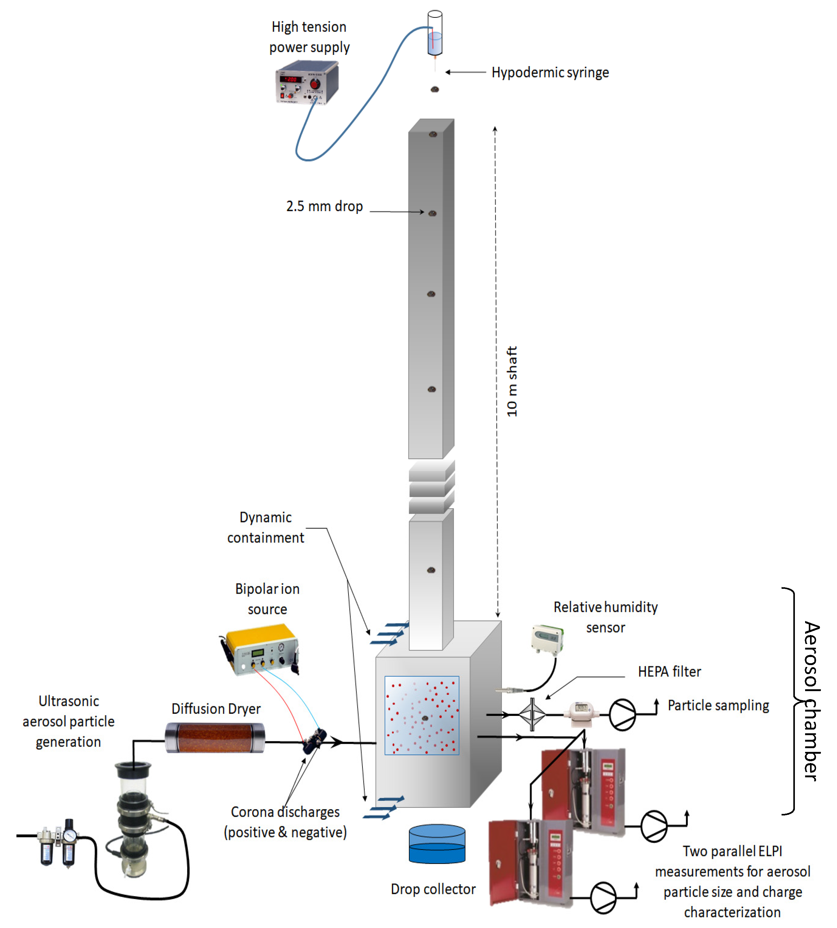
2. The Experimental Setup

The collection efficiency measurements presented in this paper were performed in the BERGAME chamber. This experimental setup, shown in Figure 1, was initially designed by Quérel. [29] and then supplemented to control and measure the respective electrical charges of the drops and aerosols [42,43]. The system comprises three parts, a drop generator, a freefall shaft, and an aerosol chamber, each detailed below.

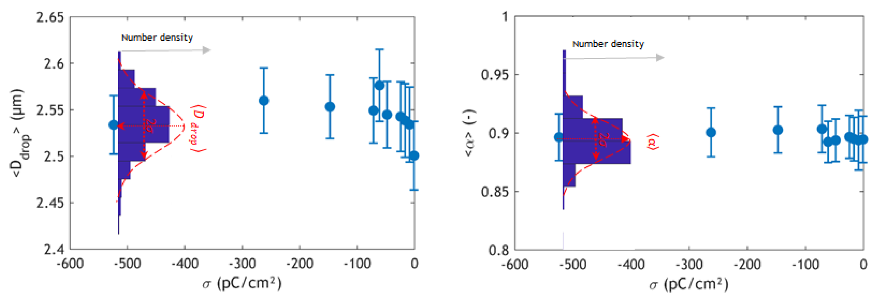
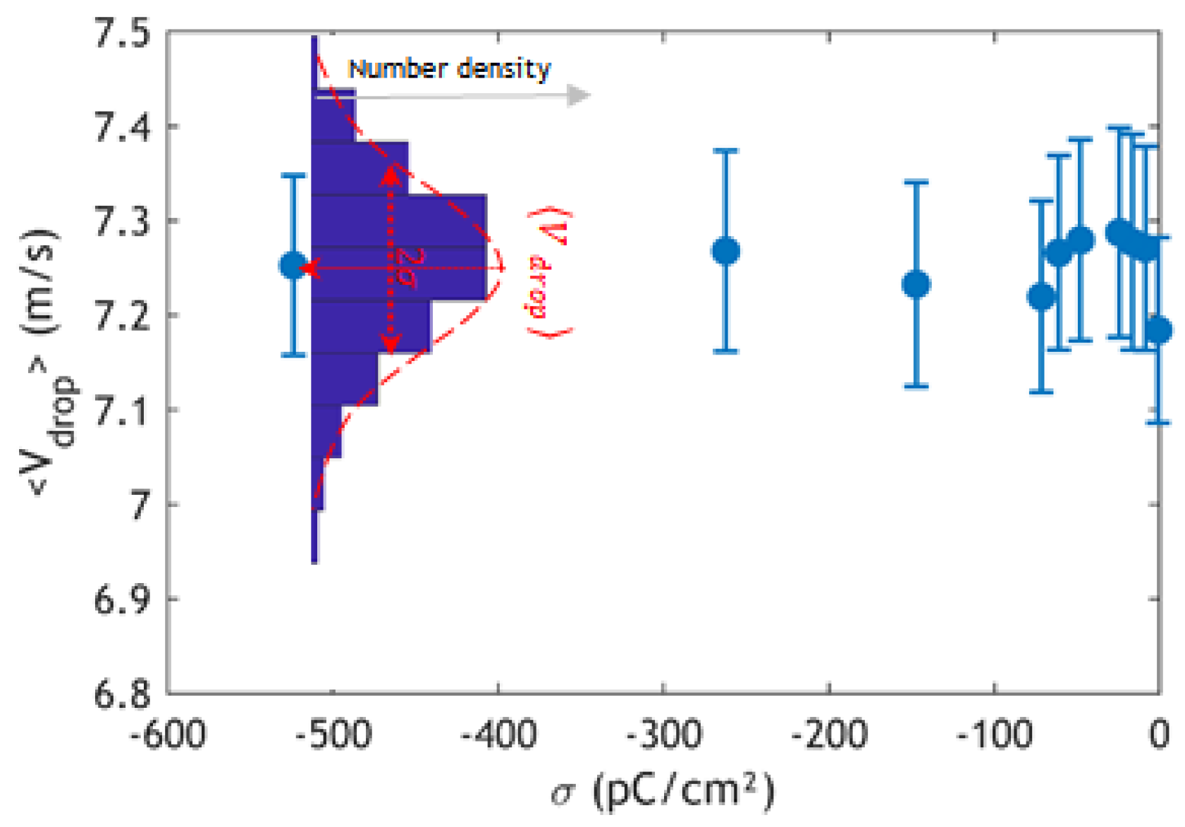
2.1. The Drop Generator

The device used to produce monodispersed drops comprises a hypodermic syringe connected to a cylindrical tank with an overflow. This overflow system maintains a constant water level in the tank and therefore constant pressure in the syringe. This system produces very weakly dispersed drops (standard deviation close to 0.1 mm) with a very stable frequency. The diameters ( D d r o p ), velocities ( V d r o p ), and axis ratios ( α ) of drops were measured in the aerosol chamber (i.e., after 10 m in the freefall shaft) using double-flash shadowgraphy for the velocity (Figure 2). For the non-spherical drops, we adopted the notion of a diameter equivalent to a sphere. As 2.5 mm drops remain symmetrical with respect to the vertical axis, their diameter can be assessed by measuring the surface of the shadow of the drop on the sensor [32].
The electric charge of the drops was controlled by connecting the water tank to a high-voltage power supply ( U   <   10   kV ). The drop electric charge control system and the drop charge measurements are detailed in Sow and Lemaitre [42,43].

2.2. The Freefall Shaft

To replicate raindrops in nature, the drops produced by this generation system are gravitationally accelerated over 10 m so that they attain their terminal velocity and equilibrium axis ratio. According to Wang and Pruppacher [51], this height is sufficient for drops with 2.5 mm diameter to reach their terminal velocity (i.e., 7.3 m·s−1 [52]). This was, however, verified. In addition, we ensured that the electric potential applied to the water in the syringe did not influence the size of the drops (as the electric charge produced by charging the liquid coming out of the syringe could potentially favor the release of drops, producing smaller drops), their terminal velocity (as they fall within the Earth’s electric field) or their equilibrium axis ratios. As stated in the introduction, 2.5 mm diameter drops falling at their terminal velocity oscillate [35,53] and therefore have a flattened spheroid shape. Zrnic et al. [54] suggest the possibility of charge build-up in the areas of the drop where the radius of curvature is larger, which would amplify its deformations. The influence of electric potential applied to the syringe on these three parameters is detailed in Appendix A. No significant influence of the electrical potential is noted from these measurements.
Figure 3 shows that after a 10 m free fall, the drops that penetrate into the aerosol chamber are representative of free-falling drops at terminal velocity (the measured velocities and axis ratios are in line with theoretical models and previous measurements).

2.3. The Aerosol Chamber

The collection chamber in the BERGAME experiment is a 1 meter high stainless steel cube ( H = 1   m ) with a 0.8 × 0.8 m2 square cross-section. It has two circular openings (one at the top and one at the bottom) for drops to pass through. Air flow was laminarized and filtered with a high-efficiency particulate air (HEPA) filter to provide dynamic containment of the aerosol chamber [60]. These flows were dimensioned at each of the orifices to prevent the laboratory, the freefall shaft, and the drop collector from being contaminated by aerosols injected into the aerosol chamber. The aerosol chamber has three portholes for measuring the size, velocity, and axis ratio of the drops as they pass through. This system was used to measure the size, axis ratio, and velocity of the drops (Figure 2 and Figure 3) for different electric potentials applied to the syringe (Appendix A). Temperature and relative humidity in the chamber were not controlled but were precisely measured. Aerosols were produced with an ultrasonic nebulizer (Synaptec: Atlanta, GA, USA, 2400). This generator comprises a piezoelectric ceramic that nebulizes the solution in which it is immersed as it vibrates (at 2400 kHz). For the experiments described in this paper, the solution used was ultrapure water (with a conductivity of about 5 µS/cm) in which pure fluorescein sodium salt was dissolved ( C 20 H 10 N a 2 O 5 ). This molecule was selected for its high fluorescence properties (measurable up to 1 × 10 11   kg · L 1 ) and because its hygroscopic properties are well known [29]. The generator therefore produced a slightly dispersed mist of droplets that was first dried by mixing with dry air, then using a diffusion dryer specially designed to produce a dry aerosol. The geometric standard deviation of aerosols produced by the nebulizer was 1.3 [29]. Dry particles of different sizes can be produced by varying the fluorescein sodium salt concentration in the solution in the generator. Once dried, the aerosols were neutralized using a bipolar ion source (EAN 581, Topas). This system comprises two corona ion sources of opposite polarity that can be adjusted separately. Each of the discharges produces an ionic current of up to 150 µA, and the ions produced were mixed with the aerosol flows in a mixing chamber. When they leave the mixing chamber, the aerosols therefore have a charge state that depends on the electric voltage applied to each of the discharges. In the present article, these voltages are set to neutralize the aerosol particles. Two electrical low pressure impactors (ELPIs, DEKATI, Figure 1) simultaneously and continually took samples from the aerosol chamber in order to simultaneously determine the particle size distribution and characterize their charge [61]. One of these two ELPIs functioned with its corona charger turned off and therefore measured the current left on each impaction stage by the charged particles. The other ELPI was used with its charger turned on and measured the size distribution of particles in the aerosol chamber. The ratio of these two values was used to determine the mean charge of the aerosols in the aerosol chamber ( < q a p > ). The mass concentration of particles in the aerosol chamber was determined through constant sampling, by the HEPA filter, and then analyzed via fluorescence spectrometry ( [ C 20 H 10 N a 2 O 5 ] c h a m b e r ). The drops were collected when leaving the aerosol chamber, and their fluorescein concentration was measured also via fluorescence spectrometry ( [ C 20 H 10 N a 2 O 5 ] d r o p ).
All these measurements were used to determine the efficiency with which aerosols particles are collected by raindrops. As previously introduced, this parameter can be defined as the ratio between the mass of fluorescein salt in the drops ( M C 20 H 10 N a 2 O 5 d r o p ) and in the volume it swept ( M C 20 H 10 N a 2 O 5 d r o p ). For each measurement point, almost 250 drops were collected in order to ensure statistical convergence of the collection efficiency.
E ( d a p , D d r o p , R H , < q a p > , Q d r o p ) = M C 20 H 10 N a 2 O 5 d r o p M C 20 H 10 N a 2 O 5 s w e p t = π 6 D d r o p 3 [ C 20 H 10 N a 2 O 5 ] d r o p π 4 D d r o p 2 . H [ C 20 H 10 N a 2 O 5 ] c h a m b e r = 2 D d r o p [ C 20 H 10 N a 2 O 5 ] d r o p 3 H [ C 20 H 10 N a 2 O 5 ] c h a m b e r
To calculate the collection efficiency (Equation (5)), the mass concentration of sodium fluorescein aerosols was determined on continuous sampling from a high-efficiency particulate air filter in the chamber. However, this mass concentration was also evaluated using the ELPI measurement. If a difference of more than 5% was observed between these two concentrations, the efficiency measurement was rejected because it meant that the particles were not made of pure fluorescein, that they were hollow from drying too quickly, or that they were non-spherical [62,63].

3. Results and Discussion

During this measurement campaign, the collection efficiencies are measured as a function of
the size and charge of the aerosol particles,
the size and charge of the drops, and
the relative humidity in the aerosol chamber.
The initial intention was to characterize the influence of the electrical charge of drops upon the efficiency with which they collect neutralized submicron aerosols. Indeed, the measurements of Lai et al. [22] display a rapid increase in the collection efficiency when the surface charge density on the drop increases. The authors explain this observation by the polarization of the particle in the electric field produced by the drop. This polarization then induces an attractive force on the particle. We intended to quantify this mechanism based on new data.
As suggested by Lai et al., the electrical charge of the drop is represented by the surface charge density on the drop (σ, ratio between the charge and surface of the drop, assuming that it is spherical) and not by the total charge to represent the results (Table 1), as is usually the case for perfect conductors. Indeed, Davis [64] showed that although a raindrop is a dielectric medium, considering a conductivity of 5   µ S . c m 1 and a dielectric constant of 81, the charge of relaxation time of water is about 1 × 10 6   s . It is almost three orders of magnitude shorter than the interaction time between the aerosol particles and the drop ( 8 × 10 4   s , time for an aerosol particle to pass around the drop—evaluated from PIV measurement). Consequently, using electrostatic solutions for dielectric spheres with finite dielectric conductivities, he showed that water drops could be considered conducting spheres.
In Table 1, the first column reports the mean aerodynamic diameter ( < d aero > ) of the aerosol continually characterised in the aerosol chamber using an ELPI. This aerodynamic diameter is then converted into a physical diameter [65], assuming a spherical particle shape ( d a p ):
d a p 2 C c ( d a p ) · ρ a p = d a e r o 2 C c ( d a e r o ) · ρ 0 .
This implicit equation is solved iteratively. Terms Cc, ρ0, and ρ a p are, respectively, the Cunningham coefficient, the water density, and the density of the sodium fluorescein aerosol [29]. Figure 4 below displays all the measurements performed as a function of the surface charge density on the drop. These data were compared with the measurements of Wang and Pruppacher [16] performed for a neutral aerosol and drops of the same size and also neutral.
This figure shows highly scattered results that lack coherence without any dependence on the drops’ surface charge density. No symmetry is observed between the positive and negative charge densities on the drop, and the measurements seem to fluctuate erratically. However, this variability cannot be linked to the measurement uncertainties, which are much lower than this dispersion. It therefore seems that another physical process should explain this variability. These same results are presented in Figure 5 as a function of relative humidity measured in the aerosol chamber.
Figure 5 shows a clear organization of measurements as a function of relative humidity. Furthermore, this representation now displays a consistency between our measurements and those of Wang and Pruppacher [16]. Moreover, for both of the aerosol sizes investigated in the article, no influence of the drop charge is observed on the collection efficiency. This seems to indicate that the polarization of the aerosol particle produced by the surface charge on the drops does not induce any relevant attractive force on the aerosol.
At first sight, it is surprising that the increase of the surface charge on the drop does not induce any measurable enhancement of the collection efficiency, whereas in the same range of aerosol particle size, Lai et al. [22] measured a four-fold increase. As previously stated, Lai et al. [22] attribute this increase to a polarization of the particle in the electric field produced by the drop. This polarization is by definition linked to the dielectric constant of the particles. In Lai et al.’s experiments, the particles consisted of silver chloride, which has a dielectric constant close to 120 [66], while sodium fluorescein salt has a dielectric constant around 20 [67]. From these dielectric constant differences, we can evaluate from Davis simulations [64] that the induction force applied on silver chloride particles is 8 times greater than it is on sodium fluorescein ones. This difference in the dielectric constant may thus explain why, in the present article, no measurable effect of the surface charge on the drop is measured on the collection efficiency.
In contrast, although relative humidity only varies slightly between measurements (the standard deviation for relative humidity measured during the experiments for 0.49 µm diameter aerosols is only 2%, and 0.42% for 0.3 µm aerosols; Table 1), this slight variation seems to have a major impact on collection efficiency. For aerosols with a diameter of 0.3 µm (red curve), the collection efficiency doubles for a decrease of just 1% in relative humidity. For collection efficiencies measured for aerosols of 0.49 µm in diameter (blue curve), the values seem to reach a plateau for relative humidities above 29%. However, below this value, efficiencies quickly increase as the relative humidity decreases. Therefore, the collection efficiency triples for a variation of just 3% in relative humidity; i.e., approximately the same dependency on relative humidity is measured for aerosols with a diameter of 0.3 µm, but no plateau is observed even if the relative humidity is higher. These results are somewhat surprising. Phoretic forces (thermophoresis and diffusiophoresis) are known to play an important role in collection [18,20]. The review paper of Santachiara et al. [20] about the contribution of phoretic effects to collection is an essential reference for identifying the respective subtleties of diffusiophoresis and thermophoresis. However, the magnitude of this variation is still a surprise, because theoretical models do not explain this result.
Various models exist for assessing the elementary contribution of phoretic effects in drop scavenging. Figure 6 compares our measurements with the models of Wang et al. [68], Young [69]—based on the Slinn and Hale’s [70] model for thermophoresis—and Davenport and Peters [71]. These three models assess the flux of particles colliding with the drop under the exclusive action of thermophoresis and diffusiophoresis (including the Stefan flow). In these models, inertia and weight of the particles are ignored while both thermophoresis and diffusiophoresis are assumed to be purely radial forces. These models are validated to evaluate the efficiency with which submicron aerosol particles are collected by droplets with a diameter smaller than 600 µm [16,21]. However, for bigger drops’ measurements from Wang and Pruppacher [16], significant differences were highlighted with these flux models [68].
Figure 6 shows that none of the three models present the same evolution as our measurements. Nevertheless, among each other, they all show similar elementary collection efficiencies following the same trends— i.e., collection efficiencies with a very low dependency, or with no dependency on aerosol size [71]—and a slow continuous increase in elementary collection efficiency when relative humidity decreases ( ~ 1.6 % . % 1 ) . This huge discrepancy, also previously highlighted [16], could suggest that one or more of the assumptions behind these three models become invalid for raindrops with a diameter bigger than 600 µm.
As one of the first, Grover et al. [18] used Lagrangian tracking of particles in the flow around drops and showed that the rear capture mechanism, which is the driving collection mechanism for submicron aerosol particles [17,32], could combine with phoretic effects “to narrow the Greenfield gap” [18]. More specifically, it seems that phoretic effects cause aerosol particles to drift from the flow streamlines following the outline of the drop’s wake to inside the wake. Once in the wake of the drop, they are re-accelerated to the rear surface of the drop under the combined effect of wake recirculating flows and gravity [17]. Unfortunately, the Lagrangian simulations of Grover et al. [18] were performed for relatively small raindrops ( D d r o p 876   µ m ), because they required simulating the flow around drops at their terminal velocity. However, at diameters exceeding 1.6 mm, raindrops oscillate, which makes it extremely difficult to model air flow around them. Therefore, to test this assumption, we used experiments to characterize flows around drops with a diameter of 2.5 mm, at their terminal velocity, using the PIV technique [50]. This optical diagnostic involves seeding a flow using very low-inertia particles, so their relaxation time is much lower than the one characterizing the fluid flow. The Stokes number ( S t , Equation (7)) is often used to characterize the ability of particles to trace the flow, and particles with a Stokes number below 0.1 are referred to as tracers [72]. Successively recording their position between two points in time ( t 1 and t 2 = t 1 + Δ t ) makes it possible to deduce the fluid’s velocity field in two dimensions if seeding is dense enough. In order to apply this technique to freefall drops at terminal velocity, the BERGAME setup was used (Figure 1). The aerosol chamber was replaced by a transparent square-section enclosure (5 cm × 5 cm) with a height of 60 cm and seeded with di(2-ethylhexyl) sebacate droplets (DEHS, ρ D E H S = 900   k g · m 3 ) generated with a multi-jet pneumatic atomizer (TSI six-jet atomizer 9306). This atomizer is applied for the substantial concentration of microdroplets it produces ( ~ 10 7   particle · c m 3   ).
The Stokes number distribution (Equation (7)) for these microdroplets is presented in Figure 7. This measurement was based on the distribution of aerodynamic diameters measured using an aerodynamic particle sizer (APS TSI SPECTROMETER 3321). This measurement shows the very low inertia of the seeded particles ( S t < 0.1 ).
S t = U , D d r o p   C c ,   d a e r o   ρ 0   d a e r o 2 9   η a i r   D d r o p
The drops were detected passing through the camera’s field of view using a fork optical sensor, which triggers the acquisition of two images with a Δ t time lapse between flashes. A specific optical configuration was used to limit the camera’s depth of field as much as possible and only observe the particles in the vertical plane, including the drop’s axis of symmetry. The particle shadow velocimetry technique was used to do this. The camera (HiSense Neo, 2560 × 2160 pixels, 16 bit) was fitted with a macro lens (Canon MP-E 65 mm f/2.8 1 − 5x Macro), and the flow was backlit using a fluorescent screen excited by a pulsed laser, which freezes the flow on each image (with a 9 ns pulse duration). This setup prevented the depth of field from being limited by the thickness of the light sheet, as would be the case with conventional PIV optical systems [41,73], but instead by the lens’s depth of field—around 70 µm, depending on the manufacturer. This system was used to record a series of image pairs. The series was filtered in order to only keep the images that include the drop’s vertical axis; this selection was performed based on the contrast of the drop contour on the image.
Since our aim was to characterize air flows around the drop at terminal velocity, in the frame of reference of the drop, its center coordinates were detected on each of the images, and the second image in each pair was translated in order to make the center of the drop overlap on each frame. The typical oscillation period for a 2.5 mm drop ( T o s c i   =   1 f o s c i = 12   m s ;   f o s c i = 85   H z [35]) is significantly longer than the time between the two frames ( Δ t = 9   µ s ), so the drop contours overlap perfectly on each of the images repositioned around the drop.
The PIV method used was an adaptive correlation algorithm with variable interrogation window shape and size, making it possible to follow both the contours of the droplet—which are first masked—and the flow velocity gradients [74]. Figure 8 shows an example of flow measurement around a 2.5 mm diameter drop under gravitational acceleration from a height of 10 m. The color code is the gas velocity module around the drop, and the flow streamlines are superimposed on this color code. These measurements were taken under atmospheric pressure, temperature, and relative humidity ( T a i r = 20   C   and R H = 49 % ).
Upstream of the drop, purely vertical flow is observed, with a module very close to the drop’s terminal velocity ( V = V y · e y ~ U , D d r o p · e y ). As they approach the drop, the streamlines embrace it. Below the drop’s equator ( θ A > 65 ) the streamlines converge together and the flow reaccelerates (in the boundary layer, velocity even exceeds the terminal velocity of the drop). Finally, we observe a flow separation at the point annotated S in Figure 8 ( θ s ~ 76 , subcritical separation). Beyond this separation point ( θ s > 76 ), the boundary layer is completely separated from the drop. In this wake, the velocities measured are very low ( < 1   m · s 1 ), whereas upstream of the drop, the flow measured is perfectly symmetrical around the vertical axis of the drop (dotted line in Figure 8); dissymmetrical and unsteady recirculating flows, very similar to the observations of Saylor and Jones [75] are observed in the wake. For drops with the same Reynolds number, Saylor and Jones observed vortex shedding, which seems to be the case with our measurements.
A few “streamlines” can be seen in red in this area, which penetrate the drop’s wake and then come into contact with the drop’s rear face. Strictly speaking, these lines are not “flow streamlines.” Fluid parcels do not penetrate the drop’s wake. They are actually “seeding particle streamlines,” i.e., curves which are tangent to each point of the particle velocity vectors. It is generally assumed that for particles with Stokes numbers below 0.1, these two notions are equivalent because the particles have very low inertia [72]. However, in the flow area where the “particle streamlines” penetrate into the drop’s wake, seeding particles cross a region with high vapor fraction gradients. The relative humidity in the wake is high because the air is sparsely renewed and continually “licks” the rear surface of the drop. However, outside these recirculating flows, the flow is very quickly renewed (>7 m·s−1, Figure 8), so relative humidity is close to atmospheric humidity (RH = 49% in Figure 8). This high vapor fraction generates a pure diffusiophoresis force. In this specific configuration, the particles do not experience Stefan flow because the streamlines are far away from the drop interface, which causes this flow. Therefore, in this configuration, diffusiophoresis is a force exerted in the same direction as the vapor gradient, i.e., horizontally and directed towards the drop axis. Diffusiophoresis does not attract particles towards the drop but into its wake. Once they have been trapped in the drop wake, submicron particles are collected behind it.
This velocity field seems to indicate a strong link between phoretic forces and rear capture for low-inertia aerosols and for raindrop with flow separation ( R e d r o p > 20 [46]) and helps understand why none of the models cited above [68,69,71] reproduce the sharp increase in collection efficiency with decreasing relative humidity. It is not, in fact, phoretic forces as such driving collection, but rear capture (i.e., the combined action of gravity and wake recirculating flows). Phoretic forces are simply the catalyst that enables aerosols to penetrate this wake. Without modelling the wake, it is impossible to predict the sharp increase in collection efficiency we measured, which is shown in Figure 5.

4. Conclusions

While the results of this article are serendipitous, they show that phoretic forces can have a major impact on the below-cloud scavenging of submicron aerosols. We measured a considerable effect of relative humidity, with collection efficiencies doubling for every percentage point drop in relative humidity. Although this coincides with the experimental results of Wang and Pruppacher (1977), none of the models in the literature seem to predict that phoretic effects would be so significant.
By applying the PIV technique for drops falling at terminal velocity, we have also shown that very low-inertia aerosols could penetrate the wake of drops and be collected on the rear surface in a sub-saturated atmosphere.
Even though some of the moisture levels investigated in this article seem very low for rain events, it is possible to encounter rain with low relative humidity at ground level, especially at the very beginning of a rainfall event. Virga are examples of such situations. Moreover, it is expected that the compelling between phoretic effect and rear capture could also be activated at higher relative humidities for smaller raindrops for two reasons. First, for smaller drops ( R e d r o p < 130), eddies remain stuck at the rear of the drop and thus enhance rear capture [17,18,32]. Second, as the velocity of the drop is lower, the lifetime of the aerosol particles along the streamlines around the wake is longer, and as a consequence, a lower vapor gradient would be required to transport the aerosol particles to the wake region. These preliminary results and their analyses should be confirmed with complementary measurement over a wider range of relative humidities and drop sizes.
This link between phoretic effects and rear capture is still complicated to model in detail because it requires simultaneously knowing flows, species fields (to precisely calculate the pure diffusiophoresis force exerted on particles) and temperature fields (to calculate the thermophoresis force exerted on particles). These three fields are difficult to simulate, as they are linked together via Stefan flows. Moreover, a major scientific obstacle remains for drops with diameters of 1.6 mm and above at their terminal velocity that oscillate at high frequency (120 Hz [35]), which makes Navier–Stokes equations particularly difficult to solve. To overcome these difficulties, hybrid approaches are proposed [76], coupling level set methods, for dynamic analysis of the interface [77]; ghost fluid methods, to improve the capture of density and viscosity jumps at interfaces [78]; and volume-of-fluid methods, to ensure preservation of mass [79]. These hybrid methods could be used for dynamic analysis of free interfaces and are therefore adapted to simulate the oscillations of drops and their impact on air flow. Moreover, in order to model phoretic effects, implementing an evaporation model into this approach is essential for calculating the pure diffusiophoresis and thermophoresis forces at each point of the flow while precisely assessing the contribution of the Stefan flow in the flow around the drop. The model of Tanguy et al. [80] could be used for this. It considers the interface at thermodynamic equilibrium, and therefore saturated with vapor, which is then transported by flow. Finally, using these velocities, temperatures and vapor fraction fields determined theoretically, particles could be tracked around the drop at terminal velocity in a Lagrangian procedure [11]. Present measurements would be excellent candidates for the validation of such a theoretical approach.

Author Contributions

Conceptualization: P.L., M.S. and A.Q.; methodology: P.L., M.S. and A.Q.; software: P.L., A.D. and A.Q.; experimentation: P.L. and M.S.; formal analysis: P.L., A.D. and T.M.; investigation: P.L.; writing—original draft preparation: P.L.; writing—review and editing: P.L., M.M. and A.F.; supervision: P.L., M.M. and A.F.; All authors have read and agreed to the published version of the manuscript.

Funding

This research received no external funding.

Conflicts of Interest

The authors declare no conflict of interest.

Appendix A

This appendix presents an empirical examination of the influence of the electric field applied to the drop generator on the properties of drops in the aerosol chamber. For clarity, only the distribution of drop diameter, axis ratio, and velocity are displayed in Figure A1 and Figure A2 for the lower surface charge density. These figures show that the electric field applied to the drop generator has no significant effect on either the diameter of the produced drops, their aspect ratio, or their terminal velocities. None of these values vary significantly with respect to measurement uncertainties. As a consequence, any collection efficiency variation observed in this paper is probably not linked to mechanical effects indirectly associated with raindrop electrical charges.
Figure A1. Influence of surface charge density on drop morphological properties.
Atmosphere 11 01028 g0a1
Figure A2. Influence of surface charge density on drop terminal velocity.
Atmosphere 11 01028 g0a2

References

  1. Jaenicke, R. Tropospheric aerosols. In International Geophysics; Academic Press: Cambridge, MA, USA, 1993; Volume 54, pp. 1–31. [Google Scholar]
  2. Dockery, D.W.; Schwartz, J.; Spengler, J.D. Air pollution and daily mortality: Associations with particulates and acid aerosols. Environ. Res. 1992, 59, 362–373. [Google Scholar] [CrossRef]
  3. Bristow, C.S.; Hudson-Edwards, K.A.; Chappell, A. Fertilizing the Amazon and equatorial Atlantic with West African dust. Geophys. Res. Lett. 2010, 37. [Google Scholar] [CrossRef]
  4. Pruppacher, H.R.; Klett, J.D. Microstructure of atmospheric clouds and precipitation. In Microphysics of Clouds and Precipitation (Section 12.4); Springer: Dordrecht, The Netherlands, 2010. [Google Scholar]
  5. Twomey, S. Pollution and the planetary albedo. Atmos. Environ. (1967) 1974, 8, 1251–1256. [Google Scholar] [CrossRef]
  6. Hegerl, G.C.; Zwiers, F.W.; Braconnot, P.; Gillett, N.P.; Luo, Y.; Marengo Orsini, J.A.; Nicholls, N.; Penner, J.E.; Stott, P.A. Understanding and Attributing Climate Change; Cambridge University Press: Cambridge, UK, 2007. [Google Scholar]
  7. Baklanov, A.; Sørensen, J. Parameterisation of radionuclide deposition in atmospheric long-range transport modelling. Phys. Chem. Earth Part B Hydrol. Oceans Atmos. 2001, 26, 787–799. [Google Scholar] [CrossRef]
  8. Mathieu, A.; Kajino, M.; Korsakissok, I.; Périllat, R.; Quélo, D.; Querel, A.; Saunier, O.; Sekiyama, T.T.; Igarashi, Y.; Didier, D. Fukushima Daiichi–derived radionuclides in the atmosphere, transport and deposition in Japan: A review. Appl. Geochem. 2018, 91, 122–139. [Google Scholar] [CrossRef]
  9. Flossmann, A.I. Interaction of Aerosol Particles and Clouds. J. Atmos. Sci. 1998, 55, 879–887. [Google Scholar] [CrossRef]
  10. Laguionie, P.; Roupsard, P.; Maro, D.; Solier, L.; Rozet, M.; Hébert, D.; Connan, O. Simultaneous quantification of the contributions of dry, washout and rainout deposition to the total deposition of particle-bound 7 Be and 210 Pb on an urban catchment area on a monthly scale. J. Aerosol Sci. 2014, 77, 67–84. [Google Scholar] [CrossRef]
  11. Depee, A.; Lemaitre, P.; Gelain, T.; Mathieu, A.; Monier, M.; Flossmann, A. Theoretical study of aerosol particle electroscavenging by clouds. J. Aerosol Sci. 2019, 135, 1–20. [Google Scholar] [CrossRef]
  12. Jaenicke, R. Physical aspects of the atmospheric aerosol. In Chemistry of the Unpolluted and Polluted Troposphere; Springer: Dordrecht, The Netherlands, 1982; pp. 341–373. [Google Scholar]
  13. Whitby, K.T. The physical characteristics of sulfur aerosols. Atmos. Environ. (1967) 1978, 12, 135–159. [Google Scholar] [CrossRef]
  14. Slinn, W.G. Precipitation Scavenging: Some Problems, Approximate Solutions and Suggestions for Future Research; No. BNWL-SA-5062; Battelle Pacific Northwest Labs.: Richland, WA, USA, 1974. [Google Scholar]
  15. Slinn, W. Some approximations for the wet and dry removal of particles and gases from the atmosphere. Water Air Soil Pollut. 1977, 7, 513–543. [Google Scholar] [CrossRef] [Green Version]
  16. Wang, P.K.; Pruppacher, H.R. An Experimental Determination of the Efficiency with Which Aerosol Particles are Collected by Water Drops in Subsaturated Air. J. Atmos. Sci. 1977, 34, 1664–1669. [Google Scholar] [CrossRef] [Green Version]
  17. Beard, K.V. Experimental and numerical collision efficiencies for submicron particles scavenged by small raindrops. J. Atmos. Sci. 1974, 31, 1595–1603. [Google Scholar] [CrossRef] [Green Version]
  18. Grover, S.N.; Pruppacher, H.R.; Hamielec, A.E. A Numerical Determination of the Efficiency with Which Spherical Aerosol Particles Collide with Spherical Water Drops Due to Inertial Impaction and Phoretic and Electrical Forces. J. Atmos. Sci. 1977, 34, 1655–1663. [Google Scholar] [CrossRef] [Green Version]
  19. Greenfield, S.M. Rain Scavenging of Radioactive Particulate Matter from The Atmosphere. J. Meteorol. 1957, 14, 115–125. [Google Scholar] [CrossRef] [Green Version]
  20. Santachiara, G.; Prodi, F.; Belosi, F. A Review of Termo- and Diffusio-Phoresis in the Atmospheric Aerosol Scavenging Process. Part 1: Drop Scavenging. Atmos. Clim. Sci. 2012, 2, 148–158. [Google Scholar] [CrossRef] [Green Version]
  21. Dépée, A.; Lemaitre, P.; Gelain, T.; Monier, M.; Flossmann, A. Laboratory study of the collection efficiency of submicron aerosol particles by cloud droplets. Part I—Influence of relative humidity. Atmos. Chem. Phys. Discuss. 2020. in review. [Google Scholar] [CrossRef]
  22. Lai, K.Y.; Dayan, N.; Kerker, M. Scavenging of aerosol particles by a falling water drop. J. Atmos. Sci. 1978, 35, 674–682. [Google Scholar] [CrossRef]
  23. Barlow, A.K.; Latham, J. A laboratory study of the scavenging of sub-micron aerosol by charged raindrops. Q. J. R. Meteorol. Soc. 1983, 109, 763–770. [Google Scholar] [CrossRef]
  24. Pranesha, T.S.; Kamra, A.K. Scavenging of aerosol particles by large water drops: Neutral case. J. Geophys. Res. Space Phys. 1996, 101, 23373–23380. [Google Scholar] [CrossRef]
  25. Tinsley, B.A.; Rohrbaugh, R.P.; Hei, M.; Beard, K.V. Effects of image charges on the scavenging of aerosol particles by cloud droplets and on droplet charging and possible ice nucleation processes. J. Atmos. Sci. 2000, 57, 2118–2134. [Google Scholar] [CrossRef]
  26. Dépée, A.; Lemaitre, P.; Gelain, T.; Monier, M.; Flossmann, A. Laboratory study of the collection efficiency of submicron aerosol particles by cloud droplets. Part II—Influence of electric charges. Atmos. Chem. Phys. Discuss. 2020. in review. [Google Scholar] [CrossRef]
  27. Grover, S.N.; Beard, K.V. A Numerical Determination of the Efficiency with which Electrically Charged Cloud Drops and Small Raindrops Collide with Electrically Charged Spherical Particles of Various Densities. J. Atmos. Sci. 1975, 32, 2156–2165. [Google Scholar] [CrossRef]
  28. Cherrier, G.; Belut, E.; Gerardin, F.; Tanière, A.; Rimbert, N. Aerosol particles scavenging by a droplet: Microphysical modeling in the Greenfield gap. Atmos. Environ. 2017, 166, 519–530. [Google Scholar] [CrossRef]
  29. Quérel, A.; Lemaitre, P.; Monier, M.; Porcheron, E.; Flossmann, A.I.; Hervo, M. An experiment to measure raindrop collection efficiencies: Influence of rear capture. Atmos. Meas. Tech. 2014, 7, 1321–1330. [Google Scholar] [CrossRef] [Green Version]
  30. Kerker, M.; Hampl, V. Scavenging of Aerosol Particles by a Failing Water Drop and Calculation of Washout Coefficients. J. Atmos. Sci. 1974, 31, 1368–1376. [Google Scholar] [CrossRef]
  31. Vohl, O.; Mitra, S.; Wurzler, S.; Diehl, K.; Pruppacher, H. Collision efficiencies empirically determined from laboratory investigations of collisional growth of small raindrops in a laminar flow field. Atmos. Res. 2007, 85, 120–125. [Google Scholar] [CrossRef]
  32. Lemaitre, P.; Querel, A.; Monier, M.; Menard, T.; Porcheron, E.; Flossmann, A.I. Experimental evidence of the rear capture of aerosol particles by raindrops. Atmos. Chem. Phys. Discuss. 2017, 17, 4159–4176. [Google Scholar] [CrossRef] [Green Version]
  33. Ladino, L.A.; Stetzer, O.; Hattendorf, B.; Günther, D.; Croft, B.; Lohmann, U. Experimental Study of Collection Efficiencies between Submicron Aerosols and Cloud Droplets. J. Atmos. Sci. 2011, 68, 1853–1864. [Google Scholar] [CrossRef]
  34. Ardon-Dryer, K.; Huang, Y.-W.; Cziczo, D.J. Laboratory studies of collection efficiency of sub-micrometer aerosol particles by cloud droplets on a single-droplet basis. Atmos. Chem. Phys. Discuss. 2015, 15, 9159–9171. [Google Scholar] [CrossRef] [Green Version]
  35. Szakáll, M.; Diehl, K.; Mitra, S.K.; Borrmann, S. A Wind Tunnel Study on the Shape, Oscillation, and Internal Circulation of Large Raindrops with Sizes between 2.5 and 7.5 mm. J. Atmos. Sci. 2009, 66, 755–765. [Google Scholar] [CrossRef]
  36. Bringi, V.N.; Chandrasekar, V.; Hubbert, J.; Gorgucci, E.; Randeu, W.L.; Schoenhuber, M. Raindrop Size Distribution in Different Climatic Regimes from Disdrometer and Dual-Polarized Radar Analysis. J. Atmos. Sci. 2003, 60, 354–365. [Google Scholar] [CrossRef]
  37. Volken, M.; Schumann, T. A Critical review of below-cloud aerosol scavenging results on Mt. Rigi. Water Air Soil Pollut. 1993, 68, 15–28. [Google Scholar] [CrossRef]
  38. Laakso, L.; Grönholm, T.; Rannik, Ü.; Kosmale, M.; Fiedler, V.; Vehkamäki, H.; Kulmala, M. Ultrafine particle scavenging coefficients calculated from 6 years field measurements. Atmos. Environ. 2003, 37, 3605–3613. [Google Scholar] [CrossRef]
  39. Chate, D.; Pranesha, T. Field studies of scavenging of aerosols by rain events. J. Aerosol Sci. 2004, 35, 695–706. [Google Scholar] [CrossRef]
  40. Depuydt, G. Etude Expérimentale in situ du Potentiel de Lessivage de L’Aérosol Atmosphérique par les Precipitations. Ph.D. Dissertation, Institut National Polytechnique de Toulouse, Toulouse, France, 2013. [Google Scholar]
  41. Querel, A.; Monier, M.; Flossmann, A.I.; Lemaitre, P.; Porcheron, E. The importance of new collection efficiency values including the effect of rear capture for the below-cloud scavenging of aerosol particles. Atmos. Res. 2014, 142, 57–66. [Google Scholar] [CrossRef]
  42. Sow, M.; Lemaitre, P. The effect of electrostatic charges on the removal of radioactive aerosols in the atmosphere by raindrops. J. Phys. Conf. Ser. 2015, 646, 012011. [Google Scholar] [CrossRef]
  43. Sow, M.; Lemaitre, P. Influence of electric charges on the washout efficiency of atmospheric aerosols by raindrops. Ann. Nucl. Energy 2016, 93, 107–113. [Google Scholar] [CrossRef]
  44. Takahashi, T. Measurement of electric charge of cloud droplets, drizzle, and raindrops. Rev. Geophys. 1973, 11, 903. [Google Scholar] [CrossRef]
  45. Adam, J.R.; Semonin, R.G. Collection Efficiency of Raindrops for Submicron Particulates; No. CONF-700601; Illinois State Water Survey: Urbana, IL, USA, 1971. [Google Scholar]
  46. Stefan, J. Über die Verdampfung aus einem kreisförmig oder elliptisch begrenzten Becken. Ann. Phys. 1882, 253, 550–560. [Google Scholar]
  47. Bowman, C.T. Course Notes on Combustion; Stanford University Course Reference Material for ME 371: Fundamentals of Combustion; Stanford University: Stanford, CA, USA, 2004. [Google Scholar]
  48. Schmitt, K.H.; Waldmann, L. Untersuchungen an Schwebstoffteilchen in diffundierenden Gasen. Z. Nat. A 1960, 15, 843–851. [Google Scholar] [CrossRef]
  49. LeClair, B.P.; Hamielec, A.E.; Pruppacher, H.R.; Hall, W.D. A Theoretical and Experimental Study of the Internal Circulation in Water Drops Falling at Terminal Velocity in Air. J. Atmos. Sci. 1972, 29, 728–740. [Google Scholar] [CrossRef]
  50. Adrian, R.J. Particle-Imaging Techniques for Experimental Fluid Mechanics. Annu. Rev. Fluid Mech. 1991, 23, 261–304. [Google Scholar] [CrossRef]
  51. Wang, P.K.; Pruppacher, H.R. Acceleration to Terminal Velocity of Cloud and Raindrops. J. Appl. Meteorol. 1977, 16, 275–280. [Google Scholar] [CrossRef]
  52. Beard, K.V. Terminal Velocity Adjustment for Cloud and Precipitation Drops Aloft. J. Atmos. Sci. 1977, 34, 1293–1298. [Google Scholar] [CrossRef]
  53. Szakáll, M.; Mitra, S.K.; Diehl, K.; Borrmann, S. Shapes and oscillations of falling raindrops—A review. Atmos. Res. 2010, 97, 416–425. [Google Scholar] [CrossRef]
  54. Zrnic, D.S.; Doviak, R.; Mahapatra, P.R. The effect of charge and electric field on the shape of raindrops. Radio Sci. 1984, 19, 75–80. [Google Scholar] [CrossRef]
  55. Andsager, K.; Beard, K.V.; Laird, N.F. Laboratory Measurements of Axis Ratios for Large Raindrops. J. Atmos. Sci. 1999, 56, 2673–2683. [Google Scholar] [CrossRef]
  56. Pruppacher, H.R.; Beard, K.V. A wind tunnel investigation of the internal circulation and shape of water drops falling at terminal velocity in air. Q. J. R. Meteorol. Soc. 1970, 96, 247–256. [Google Scholar] [CrossRef]
  57. Pruppacher, H.R.; Pitter, R.L. A semi-empirical determination of the shape of cloud and rain drops. J. Atmos. Sci. 1971, 28, 86–94. [Google Scholar]
  58. Green, A.W. An Approximation for the Shapes of Large Raindrops. J. Appl. Meteorol. 1975, 14, 1578–1583. [Google Scholar] [CrossRef]
  59. Beard, K.V.; Chuang, C. A New Model for the Equilibrium Shape of Raindrops. J. Atmos. Sci. 1987, 44, 1509–1524. [Google Scholar] [CrossRef]
  60. Mocho, V. Pollution Microbienne, Particulaire et Gazeuse d’un Espace Protégé par une ou Plusieurs Arrières de Confinement Dynamique. Ph.D. Thesis, University of Paris-Val-de-Marne, Paris, France, 1996. [Google Scholar]
  61. Glover, W.; Chan, H.-K. Electrostatic charge characterization of pharmaceutical aerosols using electrical low-pressure impaction (ELPI). J. Aerosol Sci. 2004, 35, 755–764. [Google Scholar] [CrossRef]
  62. Vehring, R.; Foss, W.R.; Lechuga-Ballesteros, D. Particle formation in spray drying. J. Aerosol Sci. 2007, 38, 728–746. [Google Scholar] [CrossRef]
  63. Hardy, D.; Walker, J.; Lemaitre, P.; Reid, J. High-Time Resolution Measurements of Droplet Evaporation Kinetics and Particle Crystallisation. Available online: https://eac2020.de/2020/07/31/id350-high-time-resolution-measurements-of-droplet-evaporation-kinetics-and-particle-crystallisation/ (accessed on 22 September 2020).
  64. Davis, M.H. Electrostatic Field and Force on a Dielectric Sphere near a Conducting Plane—A Note on the Application of Electrostatic Theory to Water Droplets. Am. J. Phys. 1969, 37, 26. [Google Scholar] [CrossRef]
  65. Kulkarni, P.; Baron, P.A.; Willeke, K. (Eds.) Aerosol Measurement: Principles, Techniques, and Applications; John Wiley & Sons: Hoboken, NJ, USA, 2011. [Google Scholar]
  66. Michel, R.; Maitrot, M.; Madru, R. Proprietes electriques du chlorure d’argent monocristallin et charge d’espace. J. Phys. Chem. Solids 1973, 34, 1039–1050. [Google Scholar] [CrossRef]
  67. Mansour, S.; Yahia, I.S.; Sakr, G.; Mansour, S.A. Electrical conductivity and dielectric relaxation behavior of fluorescein sodium salt (FSS). Solid State Commun. 2010, 150, 1386–1391. [Google Scholar] [CrossRef]
  68. Wang, P.K.; Grover, S.N.; Pruppacher, H.R. On the Effect of Electric Charges on the Scavenging of Aerosol Particles by Clouds and Small Raindrops. J. Atmos. Sci. 1978, 35, 1735–1743. [Google Scholar] [CrossRef] [Green Version]
  69. Young, K.C. The Role of Contact Nucleation in Ice Phase Initiation in Clouds. J. Atmos. Sci. 1974, 31, 768–776. [Google Scholar] [CrossRef] [Green Version]
  70. Slinn, W.G.N.; Hales, J.M. A Reevaluation of the Role of Thermophoresis as a Mechanism of In- and Below-Cloud Scavenging. J. Atmos. Sci. 1971, 28, 1465–1471. [Google Scholar] [CrossRef] [Green Version]
  71. Davenport, H.; Peters†, L.K. Field studies of atmospheric particulate concentration changes during precipitation. Atmos. Environ. (1967) 1978, 12, 997–1008. [Google Scholar] [CrossRef]
  72. Adrian, L.; Adrian, R.J.; Westerweel, J. Particle Image Velocimetry (No. 30); Cambridge University Press: Cambridge, UK, 2011. [Google Scholar]
  73. Lindken, R.; Merzkirch, W. A novel PIV technique for measurements in multiphase flows and its application to two-phase bubbly flows. Exp. Fluids 2002, 33, 814–825. [Google Scholar] [CrossRef]
  74. Wieneke, B.; Pfeiffer, K. Adaptive PIV with variable interrogation window size and shape. In Proceedings of the 5th International Symposium on Applications of Laser Techniques to Fluid Mechanics Lisbon, Lisbon, Portugal, 5–8 July 2010. [Google Scholar]
  75. Saylor, J.R.; Jones, B.K. The existence of vortices in the wakes of simulated raindrops. Phys. Fluids 2005, 17, 031706. [Google Scholar] [CrossRef]
  76. Menard, T.; Tanguy, S.; Berlemont, A. Coupling level set/VOF/ghost fluid methods: Validation and application to 3D simulation of the primary break-up of a liquid jet. Int. J. Multiph. Flow 2007, 33, 510–524. [Google Scholar] [CrossRef]
  77. Osher, S.; Fedkiw, R.; Piechor, K. Level Set Methods and Dynamic Implicit Surfaces. Appl. Mech. Rev. 2004, 57, B15. [Google Scholar] [CrossRef] [Green Version]
  78. Fedkiw, R.; Aslam, T.; Merriman, B.; Osher, S. A Non-oscillatory Eulerian Approach to Interfaces in Multimaterial Flows (the Ghost Fluid Method). J. Comput. Phys. 1999, 152, 457–492. [Google Scholar] [CrossRef]
  79. Sussman, M.; Puckett, E.G. A Coupled Level Set and Volume-of-Fluid Method for Computing 3D and Axisymmetric Incompressible Two-Phase Flows. J. Comput. Phys. 2000, 162, 301–337. [Google Scholar] [CrossRef] [Green Version]
  80. Tanguy, S.; Ménard, T.; Berlemont, A. A Level Set Method for vaporizing two-phase flows. J. Comput. Phys. 2007, 221, 837–853. [Google Scholar] [CrossRef]
Figure 1. BERGAME experimental setup.
Atmosphere 11 01028 g001
Figure 2. Measurement of the sizes, velocities, and axis ratios of drops. Δ t is the time between two flashes, Δz is the distance crossed by the drop during Δ t , S d r o p is the section of the drop, a and b are, respectively, the horizontal and vertical diameter of the drop.
Atmosphere 11 01028 g002
Figure 3. (a): correlation between drop size and velocity, and comparison with the theoretical terminal velocity established by Beard [52]. (b): Comparison of the distribution of axis ratios (bar graph in blue) measured in the aerosol chamber with mean axis ratios reported by Andsager (in grey) [55]. This area includes the mean axis ratios measured by Pruppacher and Beard [56] and the models of Pruppacher and Pitters [57], Green [58], and Beard and Chuang [59].
Atmosphere 11 01028 g003
Figure 4. Measurement of the influence of the drops’ surface charge density on the collection efficiency of submicron aerosol particles.
Atmosphere 11 01028 g004
Figure 5. Measurement of the influence of relative humidity in the aerosol chamber on the collection efficiency of drops.
Atmosphere 11 01028 g005
Figure 6. Comparison of measurements performed for this article with the various theoretical models in the literature for assessing the elementary contribution of phoretic effects—please note that in this figure, the Davenport and Peters model (1978) is independent of aerosol particle size. These simulations were performed assuming that the drop is in thermodynamic equilibrium with its environment. The drop interface temperature was determined using an enthalpy balance [4].
Atmosphere 11 01028 g006
Figure 7. Stokes number distribution of DEHS droplets used to seed the flow around drops in freefall.
Atmosphere 11 01028 g007
Figure 8. Instantaneous flow field around the drop measured using particle image velocimetry (PIV). V x is the velocity component following e x , and V y is the velocity component following e y .
Atmosphere 11 01028 g008
Table 1. Collection efficiency (E) of 2.5 mm drops as a function of charge and relative humidity for two sizes of submicron aerosols. In this table, < d a e r o > and < d a p > are respectively the mean aerodynamic and physical diameter of the aerosol particles, σ is the surface charge density on the drop, < q a p > is the mean charge of the aerosol particles, and RH is the relative humidity in the aerosol chamber. The calculation of uncertainties is detailed in the appendix of Lemaitre et al. [32].
< d a e r o > (µm) < d a p > (µm) σ (pC.cm−2) < q a p > (e) RH (%)E (-)
0.62 ± 0.02 (−5 ± 0.3) × 1020 ± 0.1 28.2 ± 0.2(6.28 ± 0.6) × 10−4
(−2.7 ± 0.1) × 10231.9 ± 0.2(2.78 ± 0.2) × 10−4
(−7.2 ± 0.4) × 10131.8 ± 0.2(3.49 ± 0.4) × 10−4
(−4.94 ± 0.2) × 10128.6 ± 0.2(4.74 ± 0.4) × 10−4
(−1.95 ± 0.1) × 10129.1 ± 0.2(4.43 ± 0.4) × 10−4
(−1.20 ± 0.1) × 10129.8 ± 0.2(3.64 ± 0.4) × 10−4
−4.5229.6 ± 0.2(5.55 ± 0.6) × 10−4
(1.17 ± 0.06) × 10127.3 ± 0.2(1.10 ± 0.1) × 10−3
0.49(2 ± 0.1) × 10132.4 ± 0.2(3.25 ± 0.2) × 10−4
(2.75 ± 0.1) × 10127.1 ± 0.2(1.60 ± 0.2) × 10−3
(6.44 ± 0.3) × 10127.4 ± 0.2(1.10 ± 0.1) × 10−3
(7.50 ± 0.4) × 10127.5 ± 0.2(1.02 ± 0.1) × 10−3
(7.50 ± 0.4) × 10132.3 ± 0.2(3.75 ± 0.2) × 10−4
(1.51 ± 0.1) × 10227.7 ± 0.2(8.39 ± 0.8) × 10−4
(2.67 ± 0.1) × 10227.6 ± 0.2(1.16 ± 0.7) × 10−3
(2.67 ± 0.1) × 10232.4 ± 0.2(3.44 ± 0.4) × 10−4
(5.31 ± 0.3) × 10227.7 ± 0.2(7.79 ± 0.7) × 10−4
0.42 ± 0.020.3(−1.44 ± 0.07) × 102 35.8 ± 0.2(7.98 ± 0.7) × 10−4
(2.75 ± 0.1) × 1020 ± 0.136.3 ± 0.2(6.55 ± 0.6) × 10−4
(5.12 ± 0.2) × 10136.4 ± 0.2(5.99 ± 0.6) × 10−4
(7.49 ± 0.4) × 10136.8 ± 0.2(4.77 ± 0.4) × 10−4
(2.67 ± 0.1) × 10236.0 ± 0.2(7.39 ± 0.7) × 10−4
(5.31 ± 0.3) × 10235.7 ± 0.2(6.91 ± 0.6) × 10−4

