Article

Formation of Clay-Rich Layers at The Slip Surface of Slope Instabilities: The Role of Groundwater

1
Departamento de Geodinámica, Universidad de Granada, 18010 Granada, Spain
2
Université Grenoble Alpes, Université Savoie Mont Blanc, CNRS, IRD, IFSTTAR, ISTerre, 38000 Grenoble, France
3
Institute of Earth Surface Dynamics, Faculty of Geosciences and Environment, University of Lausanne, 1015 Lausanne, Switzerland
4
Instituto Andaluz de Ciencias de la Tierra, CSIC-UGR, 18100 Armilla Granada, Spain
*
Author to whom correspondence should be addressed.
Water 2020, 12(9), 2639; https://doi.org/10.3390/w12092639
Submission received: 10 August 2020 / Revised: 11 September 2020 / Accepted: 16 September 2020 / Published: 21 September 2020
(This article belongs to the Special Issue Water-Induced Landslides: Prediction and Control)

Abstract

:
Some landslides around the world that have low-angle failure planes show exceptionally poor mechanical properties. In some cases, an extraordinarily pure clay layer has been detected on the rupture surface. In this work, a complex landslide, the so-called Diezma landslide, is investigated in a low- to moderate-relief region of Southeast Spain. In this landslide, movement was concentrated on several surfaces that developed on a centimeter-thick layer of smectite (montmorillonite-beidellite) clay-rich level. Since these clayey levels have a very low permeability, high plasticity, and low friction angle, they control the stability of the entire slide mass. Specifically, the triggering factor of this landslide seems to be linked to the infiltration of water from a karstic aquifer located in the head area. The circulation of water through old failure planes could have promoted the active hydrolysis of marly soils to produce new smectite clay minerals. Here, by using geophysical, mineralogical, and geochemical modelling methods, we reveal that the formation and dissolution of carbonates, sulfates, and clay minerals in the Diezma landslide could explain the elevated concentrations of highly plastic secondary clays in its slip surface. This study may help in the understanding of landslides that show secondary clay layers coinciding to their low-angle failure planes.

Graphical Abstract

1. Introduction

Groundwater interacts with soils and rocks by modifying their chemical and mineralogical properties; in the case of slope materials, this could be critical due to the reduction of shear strength in landslide materials and slip zones (e.g., [1,2,3,4]). Thus, hydrogeochemical reactions should be considered in analyses of landslides because they can locally change soil and rock properties and modify the stability of a slope. The review of [5] highlighted the potential role of hydrogeochemical studies in landslide research. These studies have provided information about the origin of groundwater and its interactions with the lithology composing the unstable slope. Other authors have also presented some examples, mostly dealing with quick clays [6], where the composition of the pore water influences the permeability and shear strength of soils and rocks (cf. [7]). Nonetheless, the application of hydrogeochemical models in landslide research is scarce in the international scientific literature, although water–rock or water–soil interaction processes are behind the instability of many slopes.
The most dramatic examples of how those processes produce unstable slopes are observed in active volcanoes, where hydrothermal alteration produces intensive rock weathering, leading to the destabilization of entire volcano flanks and finally unleashing giant debris avalanches [8,9]. There are other examples of less spectacular landslides that are driven by the chemical alteration of rocks and soil minerals but still have significant socio-economic consequences [10,11]. These landslides are those occurring at low gradients in highly populated areas of low-to moderate- relief regions, which have caused great economic losses and occasionally fatalities (e.g., [12,13,14,15,16,17]). Some of these landslides appear to be conditioned by the transformation of rocks and soil minerals into very low-permeability and high-plasticity clays. This transformation is evidenced by secondary clay-bearing layers in slip surfaces, something observed in landslides of Santa Lucia and Barbados [18], Japan [19], Italy [20], Hong-Kong [21], and particularly in the Three Gorges Reservoir region of China (e.g., [22,23,24,25]). The presence of these argillaceous layers, which are normally composed of a high proportion of clays belonging to the smectite group, poses a problem for slope stability analyses because these layers have mechanical properties that are very different from those of the slope materials. Moreover, these properties are very unfavorable from a stability point of view. High-plasticity clays, such as the members of the smectite group, considerably decrease the shear strength, thus causing landslides at very low gradients (e.g., [13,26,27]). Therefore, if these layers are not detected or considered, a given slope stability analysis will tend to overestimate the strength of the slope. One such example is the case study of this paper, the Diezma landslide (Spain). This landslide mobilized a surficial deposit due to the presence of a clay-bearing layer composed of up to 38–46% smectite [28]. The aim of this paper is to propose an explanation for the generation of the clay-bearing layer that played a key role in the failure and reactivation of this landslide. The analysis presented here complements the studies of [29] on the La Clapière landslide (France), [30] on the Super-Sauze mudslide (France), and [31] on the Ca’Lita landslide (Italy). All of these authors used simulations of water–rock interactions as a tool to characterize the origin and pathways of slope groundwater. The novelty of our study is that although we applied the same techniques, our objective is different: To understand how groundwater chemistry may produce the conditions necessary for slope instability.
The structure of the paper is as follows. We first describe the geographical-geological setting and summarize the main characteristics of the Diezma landslide according to the results of previous studies. Then, the new methods applied to the landslide in this research are explained, as well as the results obtained. The last section discusses and integrates the results of this and previous research in order to form a hypothesis on the origin of the clay-bearing layer of the Diezma landslide and its relationship with the history of that mass movement.

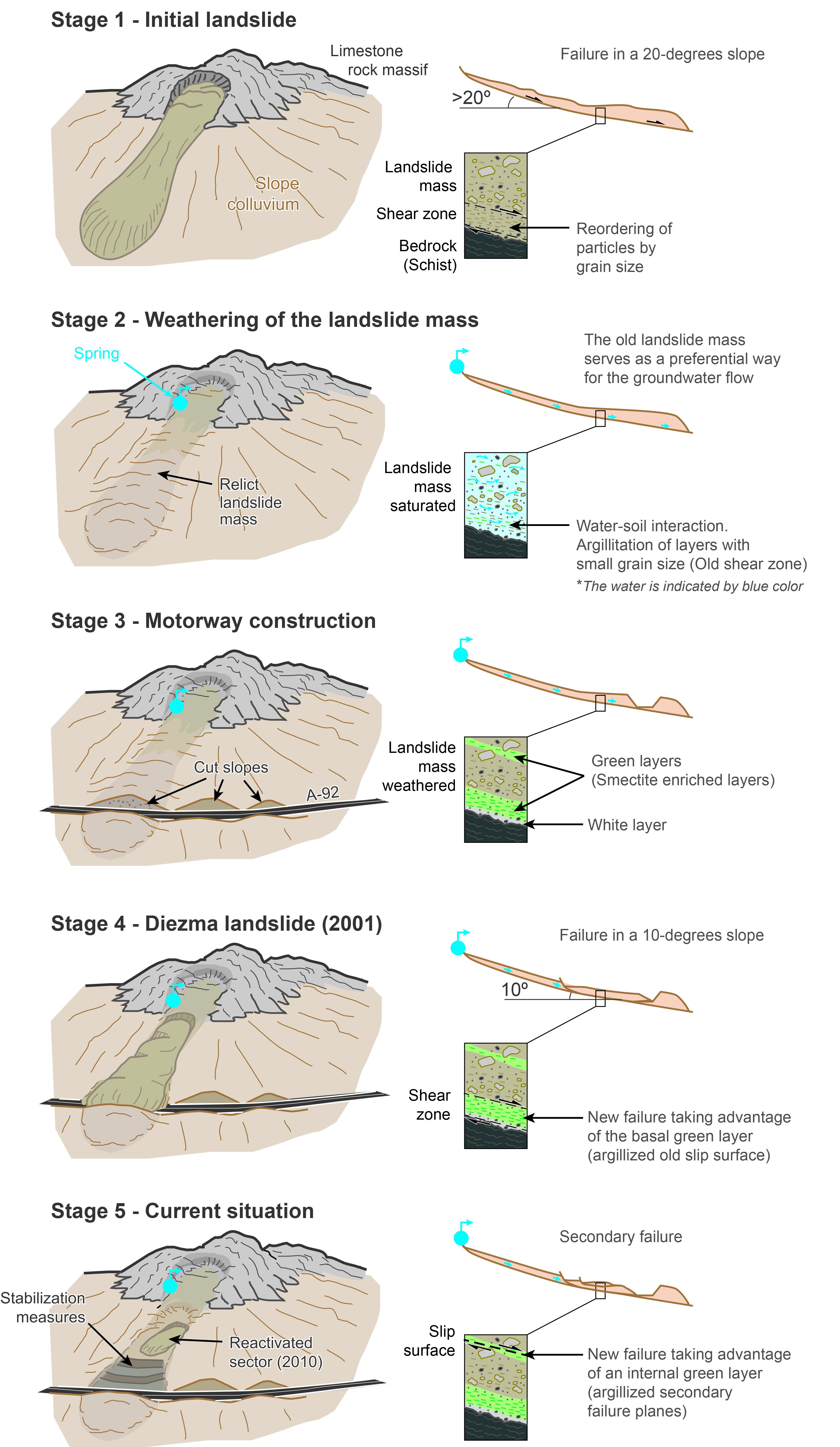
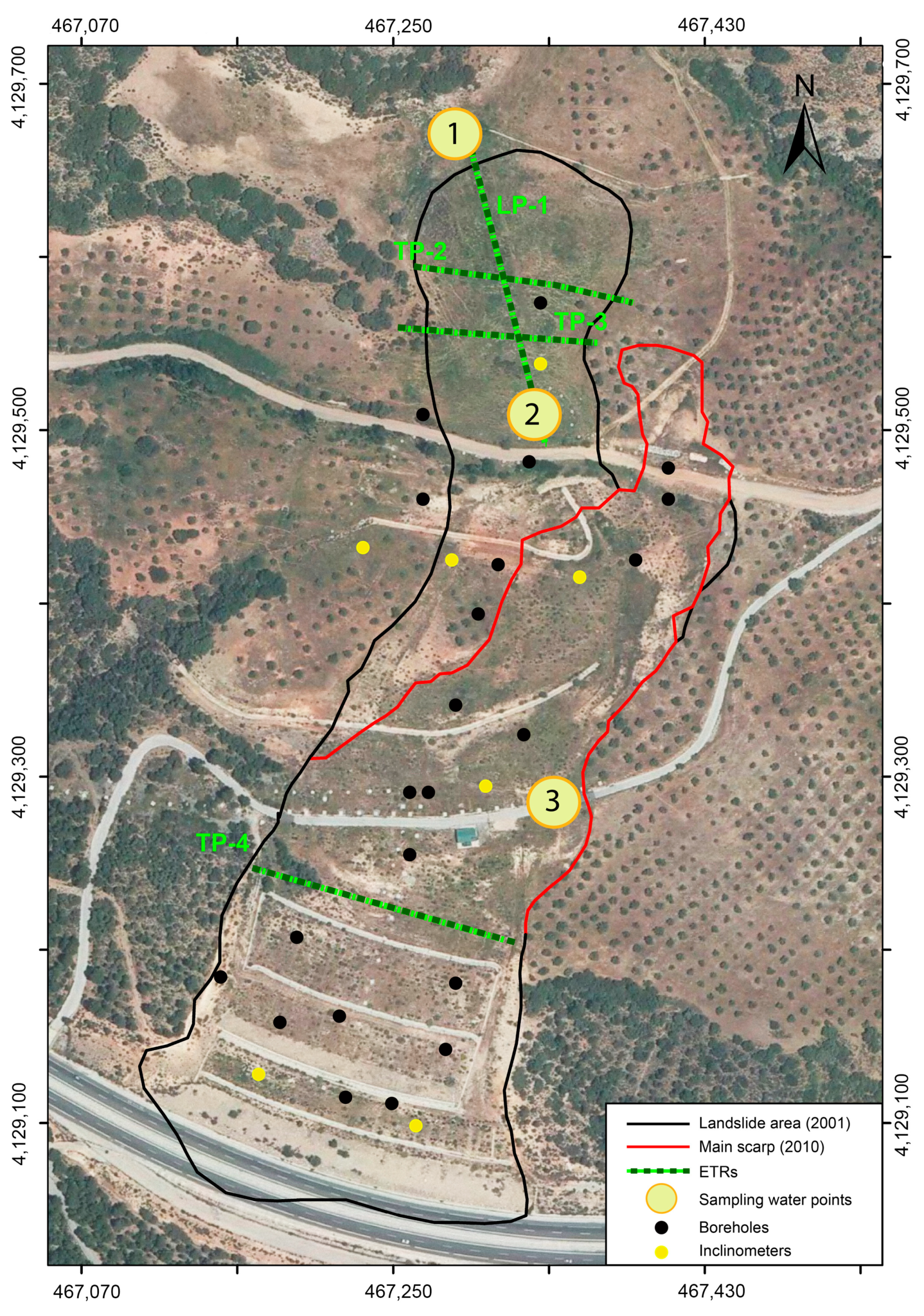
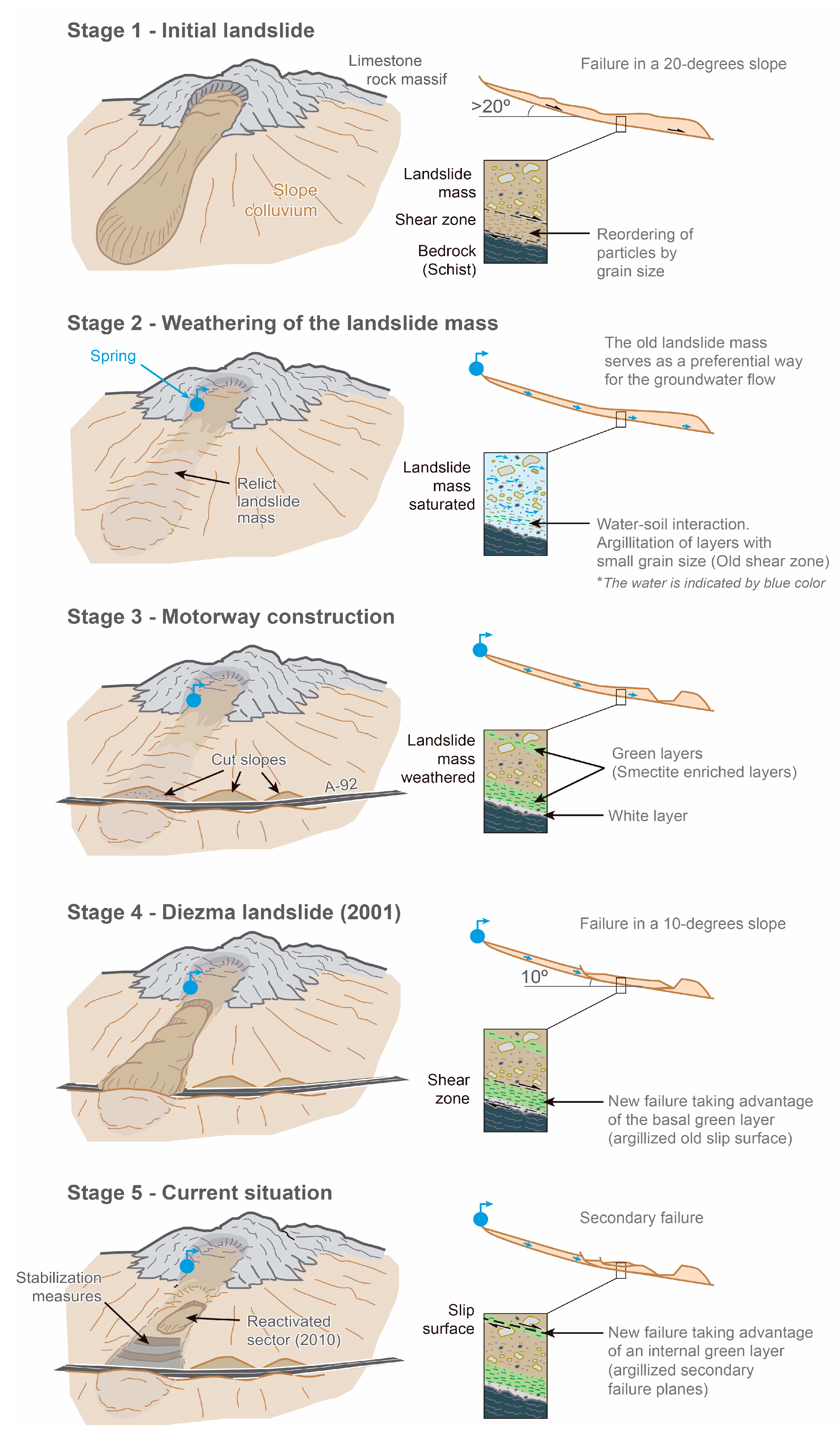
2. Geological and Geographical Setting of the Diezma Landslide

The Diezma landslide is located in a moderate-relief area of the central sector of the Betic Cordillera (SE Spain), close to the village of Diezma (Figure 1). This area, which is located at the boundary between the external (South Iberian Domain) and internal zones (Alborán Domain) of the Betic Cordillera, is affected by landslides of variable sizes and types, most of which probably represent reactivated ancient failures [11,32,33].
The Diezma landslide affects quartzite, sandstone, limestone, and dolostone blocks embedded in high-to moderate-plasticity clays, silts, and marls [11]. All of these lithologies were originally part of a flysch-type formation. This formation constitutes a siliciclastic turbidite sequence of Cretaceous–Lower Miocene age [34] and occupies an intermediate position between the South Iberian and the Alborán Domain. The flysch-type formation shows a chaotic appearance because it was intensively deformed during the Alpine orogeny. In all places where the stratigraphic sequence is complete, this formation includes sandstone blocks.
In the area of the Diezma landslide, the flysch formation is structurally superimposed over the Silurian–Triassic rocks of the Maláguide Complex (Alborán Domain), which include sandstones, conglomerates, and red limestones [35]. The carbonate rocks (Upper Jurassic limestones and dolostones) of the South Iberian Domain are thrust onto the Maláguide Complex and crop out just to the north of the Diezma landslide. These rocks show a high degree of karstification and form an unconfined karstic aquifer, which drains to the south sector. Several springs appear on the contact surface between the low-permeability flysch-like rocks and the carbonate rocks when the water table in the karstic aquifer commonly rises after a period of intense rainfall.
Regarding the hydrogeology of the landslide, three units with varying hydrogeological behaviors can be distinguished: (i) Carbonate materials from the South Iberian Domain, which have a high permeability due to karstification; this unit constitutes a free aquifer in which groundwater circulates through fissures (secondary porosity); (ii) the materials of the Flysch formation, with low permeability but affected by frequent gravitational movements and colluvial phenomena; and (iii) materials from the Maláguide Complex, which have a low permeability due to the predominance of clay and slate materials. However, this formation contains sandstones and conglomerate intercalations with medium permeability [36].
The flows provided by carbonate materials, which act as an aquifer in the region, are generally low (almost never exceed 1 L/s) although they sometimes remain constant as occurs in the spring located at the head of the landslide, at 1300 m above sea level (point 1 of our sampling, Figure 2 and Figure 3.) This flow does not even justify the recharge by direct infiltration of rainwater in the small limestone outcrop (less than 10,000 m2) associated with the spring. Therefore, sometimes there must be hidden water connections between different outcrops of materials or aquifers [37].
As mentioned above, the tectonic structure of the materials brings the clay materials from the flysch formation into contact with the carbonate aquifer materials located at a higher level. Thus, we could assimilate this situation to the existence of a constant hydraulic potential at the head of the slipped zone, which could favor a certain hidden lateral water supply from the carbonates to the sliding materials, increasing its fluid pressure much more than the simple direct infiltration of rainwater would have done.
This hypothesis of a continuous groundwater flow from carbonate materials towards the flysch formation outcropping in a lower topographically position helps to explain the time lag between the last rainy events and the moment of the slope break [11,37].

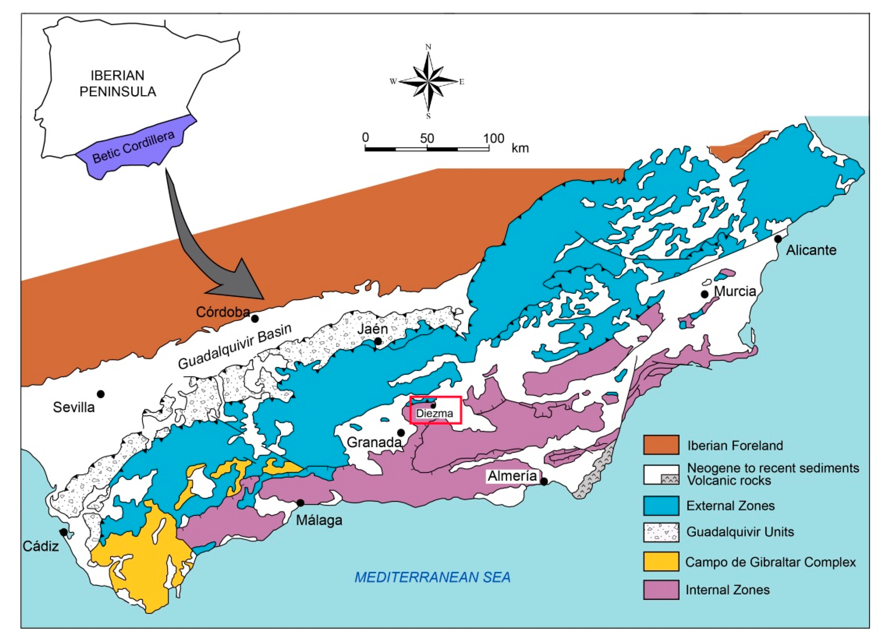
3. Characteristics of the Diezma Landslide

The Diezma landslide is considered a complex movement affecting an area of 7.76 ha, with a maximum length of 510 m and a maximum width of 205 m [32,38]. We divided the landslide body into three main sectors (Figure 2):
  • The landslide head is located on the old Granada–Almería road (CN-342). In this area, several meter-scale scarps were observed. These scarps correspond to the shallow rotational slides that have developed successively on the clay-rich rocks of the flysch formation. The impermeable characteristic of these shear surfaces favored the development of ponds at the foot of the main scarp [11].
  • The intermediate part of the landslide was formed by progressive rotational slides that produced some secondary scarps, which generated bulges with tension cracks at their crests.
  • The landslide style grades downhill from a multiple rotational slide into a proper earthflow. In the toe sector, the thickness of the mass movement in the central area is approximately 30 m.
The Diezma landslide took place on 18th March 2001, 20 days after a peak in intense rainfall that was preceded by several rainfall episodes, all of which occurred within one year. This year was wetter than average [11,32,33,39]. The observed 20-day lag time can be explained by the delay in receiving the contribution of groundwater flow from the karst aquifer [32].
Immediately after the Diezma landslide occurred, its stabilization began; an additional four lines of surface drainage systems and three lines of deep drainage wells were installed, and a barrier of anchored piles and a retaining wall at the toe of the slope were constructed [37,40]. In 2002, after the stabilization project was completed, a topographic monitoring system was installed that includes 29 benchmarks and 10 inclinometers within the landslide mass [33] (Figure 3).
However, during field investigations in 2005, it was observed that the water table was very high in the head area of the Diezma landslide, which indicated that the drainage systems in this zone were not working properly [41]. Due to this, the Diezma landslide was partially reactivated as a result of the heavy rainfall that occurred during the winter of December 2009–February 2010.
Azañón et al. [11] pointed out that the geotechnical characteristics of the material (Table 1) in the slide mass and those in the slip surface are very different. The landslide debris is heterogeneous in nature and is mainly composed of sandstone and dolostone blocks embedded in a marl–clay matrix. These materials were interpreted as a part of a surficial deposit most likely produced by a former mass movement. On the other hand, the material in the slip surface consists of a centimeter-thick smectite-rich layer. Thus, the values of the mechanical properties of the mobilized material are markedly greater than those of the slip surface (Table 1). The smectite-rich layer is highly plastic and extremely expansive (Table 1). The liquid limits estimated by [11] range from 58 to 92, while the plastic limits range from 24 to 32. The slide mass has relatively high shear strength values (c = 20 kPa and ϕp = 35°). The shear strength in the failure surface is conditioned by residual strength parameters (c = 39 kPa and ϕr = 7°). The residual friction angle of the landslide debris is also very low (ϕr = 20°). In this landslide, close to the secondary scarp, previous researchers [11] describe that the smectite-rich levels occur above a powdery white level, consisting of pure calcite with a very small grain size (Figure 4). Borehole data to which the authors of this paper have had access show that this white level is only present in the middle part of the landslide. On the other hand, the thickness of the smectite-rich layer increases toward the toe of the landslide.
Nieto et al. [28] determined the proportions of smectite in the slide mass and in the slip zone of the Diezma landslide based on the thermogravimetry of ethylene glycol (EGC)-solvated samples. Their results showed that smectite is the dominant clay mineral in the slip zone, whereas kaolinite and illite are minor minerals within the materials of the Diezma landslide. The slip zone has the greatest abundance of clay minerals compared to the materials close to this zone. For this reason, previous authors [9] suggested that water played a crucial role as a trigger and possibly as a conditioning factor taking into account the geotechnical and mineralogical characteristics of the materials involved in the Diezma landslide.
To date, the stability problems in the slope have continued, although extensive engineering measures were applied after the failures in 2001 and 2010. Recently, new monitoring programs were initiated on 2018 due to reactivations in the landslide crown. Moreover, several airborne LiDAR surveys have shown slight deformations in the toe of the slope [42]. This has indicated that the stabilization of the Diezma landslide is a complex task in which hydrogeochemical results can be used to design alternative solutions such as bio-mediated soil improvement methods (cf. [43]).

4. Methodology

First, mineralogical and geochemical methods were applied to complete the characterization of the materials observed in the slip surface. Subsequently, a geophysical survey was carried out to explore the behavior of groundwater within the landslide mass and its surroundings. Finally, by integrating all of the gathered information with previously published data, a geochemical simulation was developed to model the water–soil interactions and thus to provide a reasonable explanation for the characteristics observed in the slip zone.

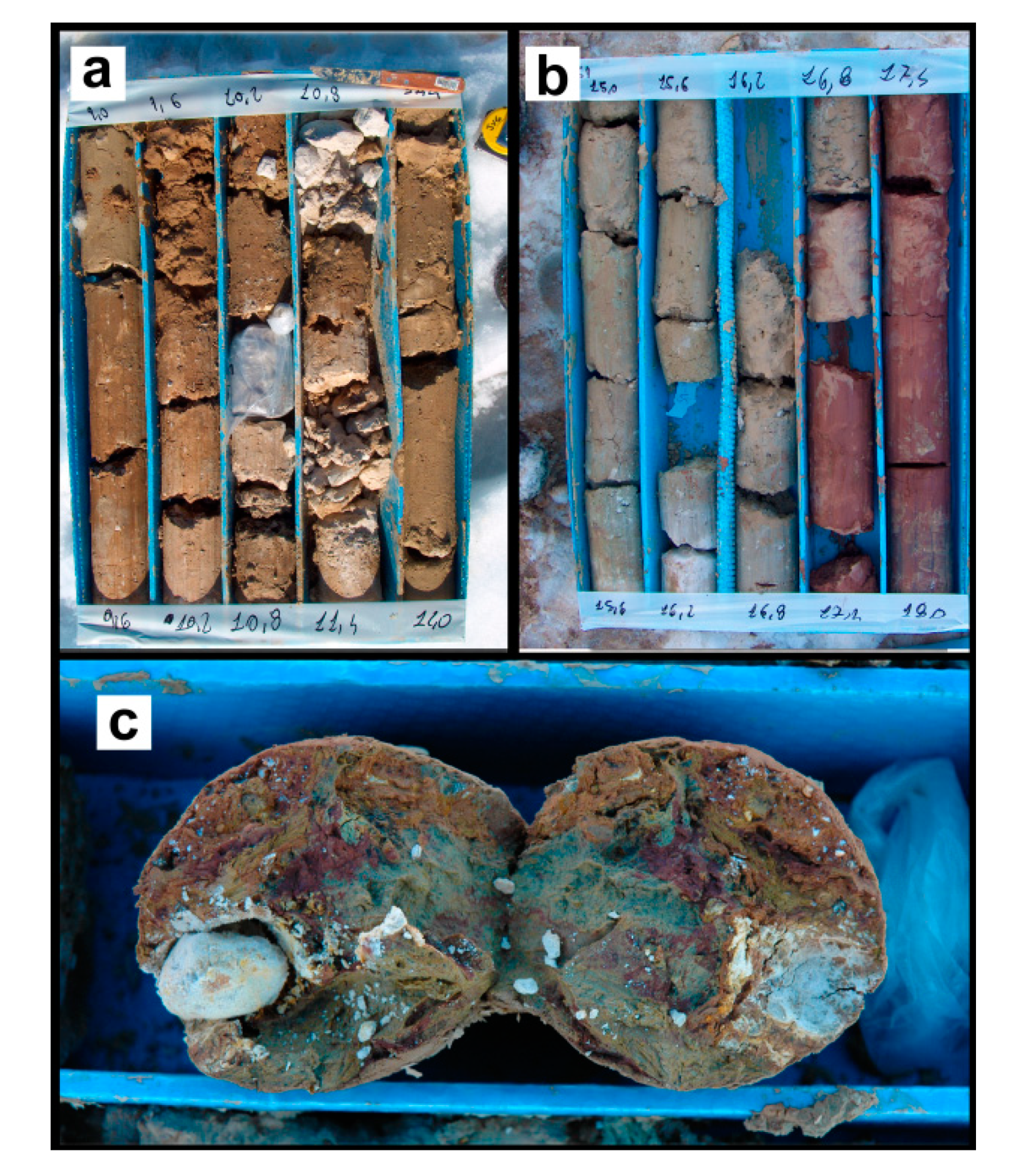
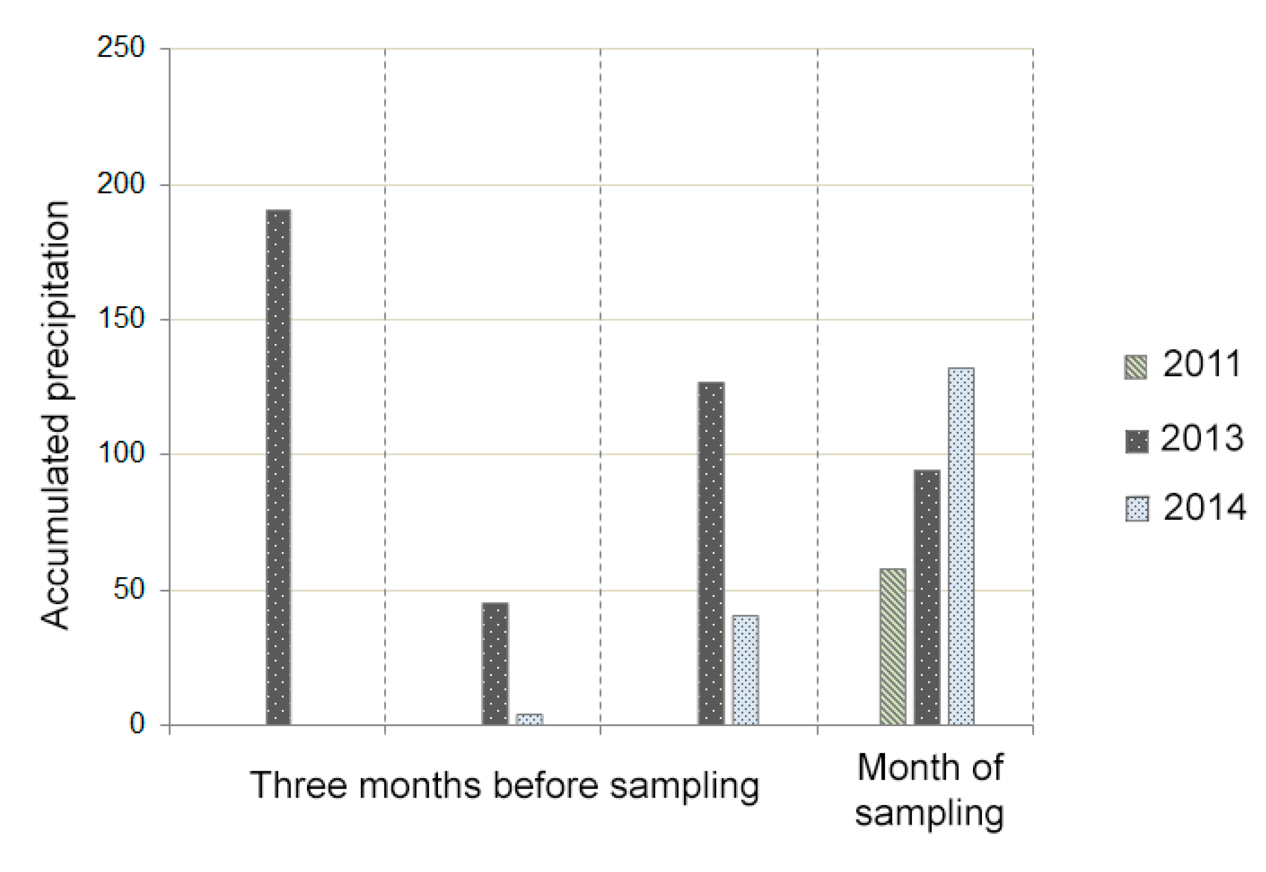
4.1. Sampling Procedure

Soil samples were collected from the failure surface. In some outcrops, it was possible to recognize a level of 1- to 3-cm-thick green clays, corresponding to the most superficial sliding surfaces. In addition, some samples were taken from the boreholes passing through the landslide. Based on borehole data and field observations, the main failure surface was found to coincide with a thin layer of clay material, whereas the mobilized mass comprised marly clay and limestone blocks. The locations of the boreholes from which the analyzed samples were collected are shown in Figure 3.
The chemical composition of the water was analyzed at three different points within the Diezma landslide numbered from 1 to 3: (1) In the spring water located at the edge of the carbonate-marly clay; (2) above the head of the landslide (at a depth of 11 m); and (3) at the lowest part of the landslide (at a depth of 27 m) (Figure 2 and Figure 3). Water was sampled in two different seasons (fall and winter) and after periods of diverse aridity/humidity conditions. Thus, the sampling scheme seeks to represent not only the chemical composition of groundwater in the slope, but also the effects of climate on the hydrochemical processes.
At each water sampling point, pH and conductivity were measured in situ using a HANNA Instruments HI 9828 Multiparameter. This equipment was checked and calibrated prior to carrying out the measurements. The concentration of cations in solution was measured using atomic absorption spectrometry inductively coupled plasma atomic emission spectrometry. The concentrations of anions (HCO3, CO3 and Cl) were analyzed by volumetric methods. The concentration of the SO4 ion was determined using spectrophotometry. For silica analysis, the heteropoly blue (also called olybdate or molybdenum blue) colorimetric method was employed (ASTM D859).

4.2. Mineralogical Characterization: X-Ray Diffractometry (XRD) and X-Ray Fluorescence (XRF)

X-ray diffractometry (XRD) is commonly used to analyze clay minerals both qualitatively and semi-quantitatively. Nevertheless, many factors must be taken into account when performing quantitative analyses. However, factors related to the semi-quantitative analyses of minerals, such as the calibration of the diffractometer and the crystallinity, orientation, and heterogeneity of the sample, are difficult to control. For the XRD analysis, mineralogical changes were studied with a PANanalytical X’Pert Pro X-ray diffractometer using disoriented powder and samples oriented by the sedimentation of the <2 µm clay fraction. The equipment settings included CuKα radiation, 45 kV, 40 mA, an exploration range of 5–70° 2θ, a step size of 0.008° 2θ, and a counting time of 10 s/step. Xpowder software [44] was used to identify mineral phases.
The smectite contents in the slide mass and the slip zone of the Diezma landslide were determined by TG analysis following the methodology developed by [28], which consisted of weight loss (WL) measurements of EG-solvated and Mg-saturated samples at temperatures ranging from 100 to 450 °C. The smectite content was calculated using the following equation: Sme% = 3.96 WL−4.05. For the X-ray fluorescence spectrometry (XRF) analysis, the fusion method, which is considered one of the methods with the highest accuracy, was used to determine the bulk chemical composition and relative abundances of the main components of the landslide materials.

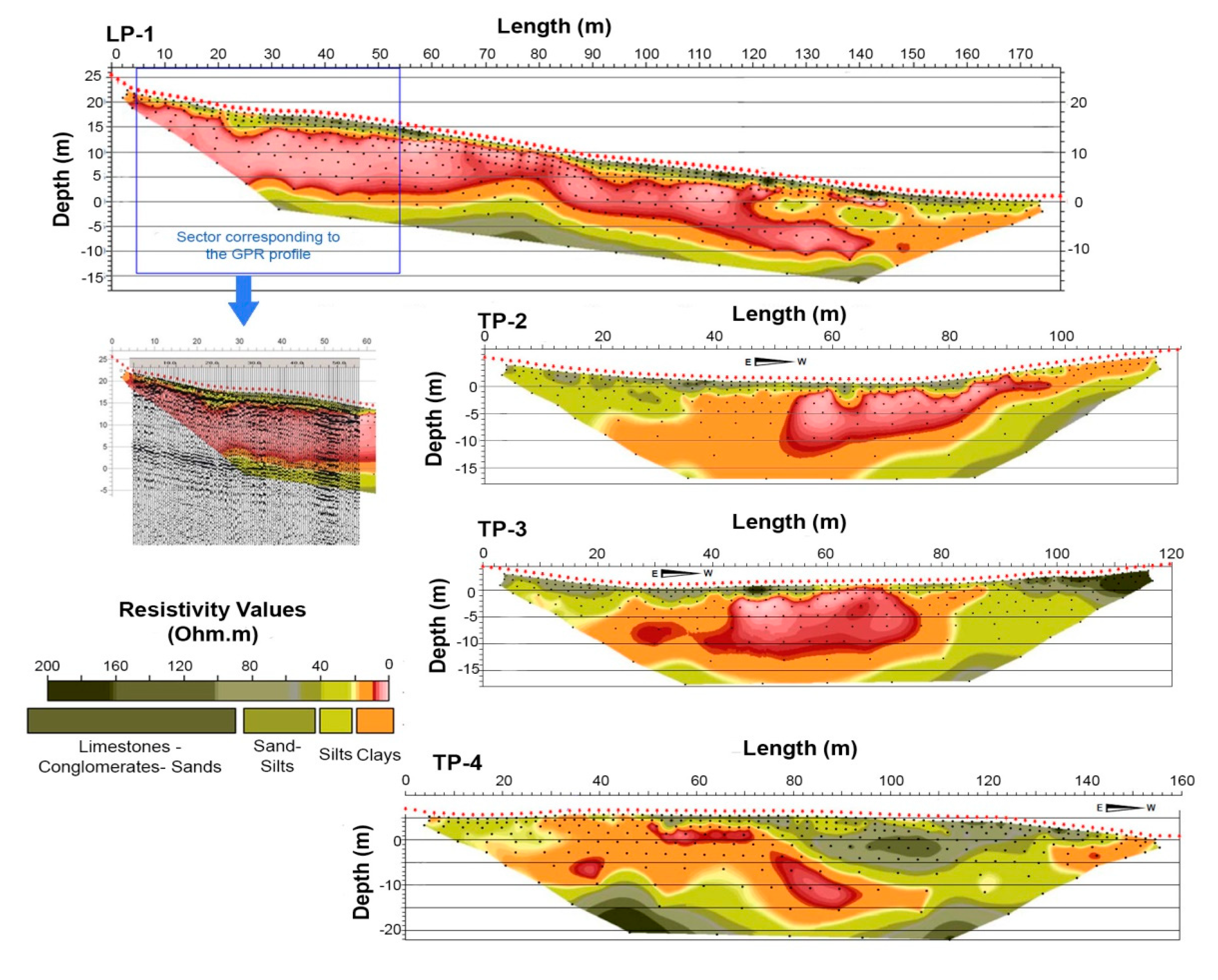
4.3. Geophysical Survey: 2D Electrical Resistivity Tomography (ERT) Profiles

To identify the water table and the role that water played in the materials involved in the Diezma landslide, high-resolution 2D electrical resistivity tomography (ERT) was used. Figure 3 shows the locations of the geoelectrical profiles obtained. Profiles LP-1, TP-2, and TP-3 are located in the head of the landslide, where the displacement is short and concentrated on a basal surface.
Profile TP-4 is located in the intermediate and lowest parts of the landslide, where the displacement is greater and concentrated in numerous scarps [45]. The LP-1 profile starts at the base of the spring water and extends to the SSE, along 180 m of topographic distance, in an area close to the main scarp. Profiles TP-2 and TP-3 are developed, from E to W, in the middle and lowest parts of the longitudinal profile, respectively.
The equipment employed was a single channel ABEM Terrameter SAS1000. All profiles were acquired using a Wenner electrode configuration with 61 electrodes connected to a multi-core cable. The depth of the model depends on the electrode spacing. In the profiles located to the N and 2 m to the S of the old road, an inter-electrode spacing of 1.5 m was chosen, as it could reach a depth of 18 m with satisfactory resolution. When necessary (i.e., in longitudinal profile), extensions (roll-along technique) were performed to increase the length of the profile to 1.5, 2 or 2.5× its standard extent. ERT data were processed using RES2DINV software, which was designed to produce an inverse model resembling the actual subsurface structure.

4.4. Geochemical Interpretative Methods: Ion-Ion Plots and Geochemical Modelling

Ion–ion plots were used to infer the possible processes affecting the hydrogeochemical evolution of the waters. Speciation-solubility, reaction-path, and mass-balance calculations were performed using the PHREEQC code [46] and the WATEQ4F thermodynamic database [47].
Inverse modelling was used to calculate the moles of minerals that must dissolve or precipitate to account for the difference in composition between an initial and a final solution. With that aim, the number of mineral phases was constrained using inverse modelling, including the potential phases involved in precipitation or dissolution processes based on a conceptual model. This model was inferred based on the general trends in the water chemical data and the saturation indices of the waters with respect to different mineral phases.

5. Results

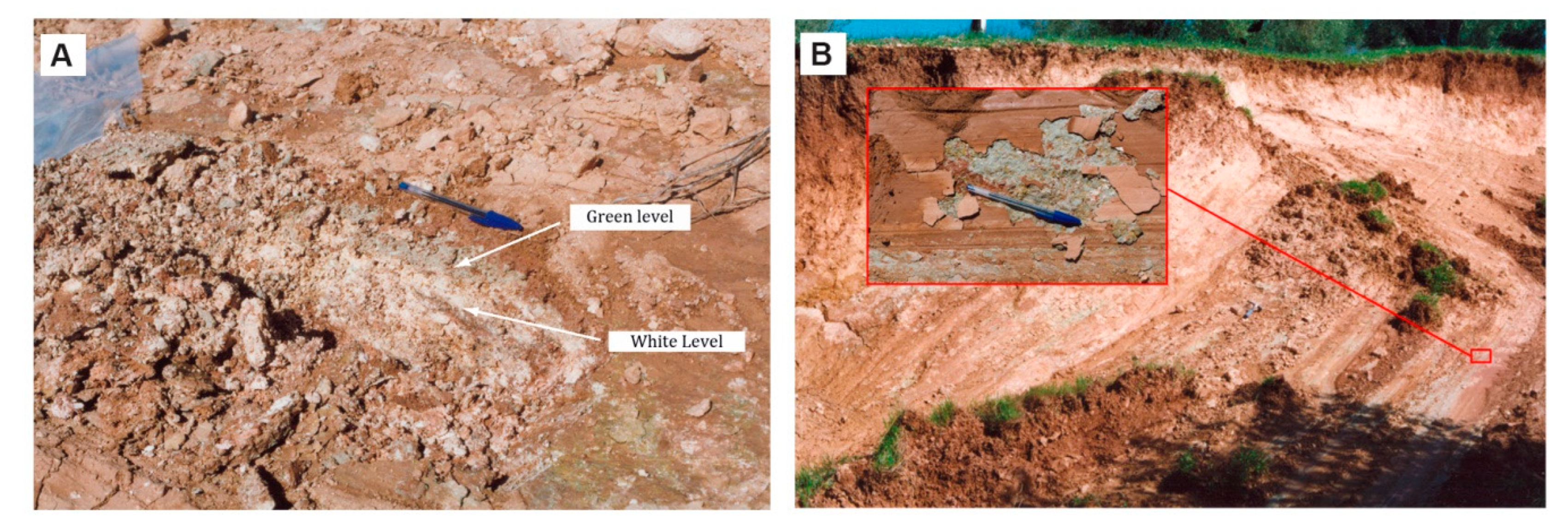
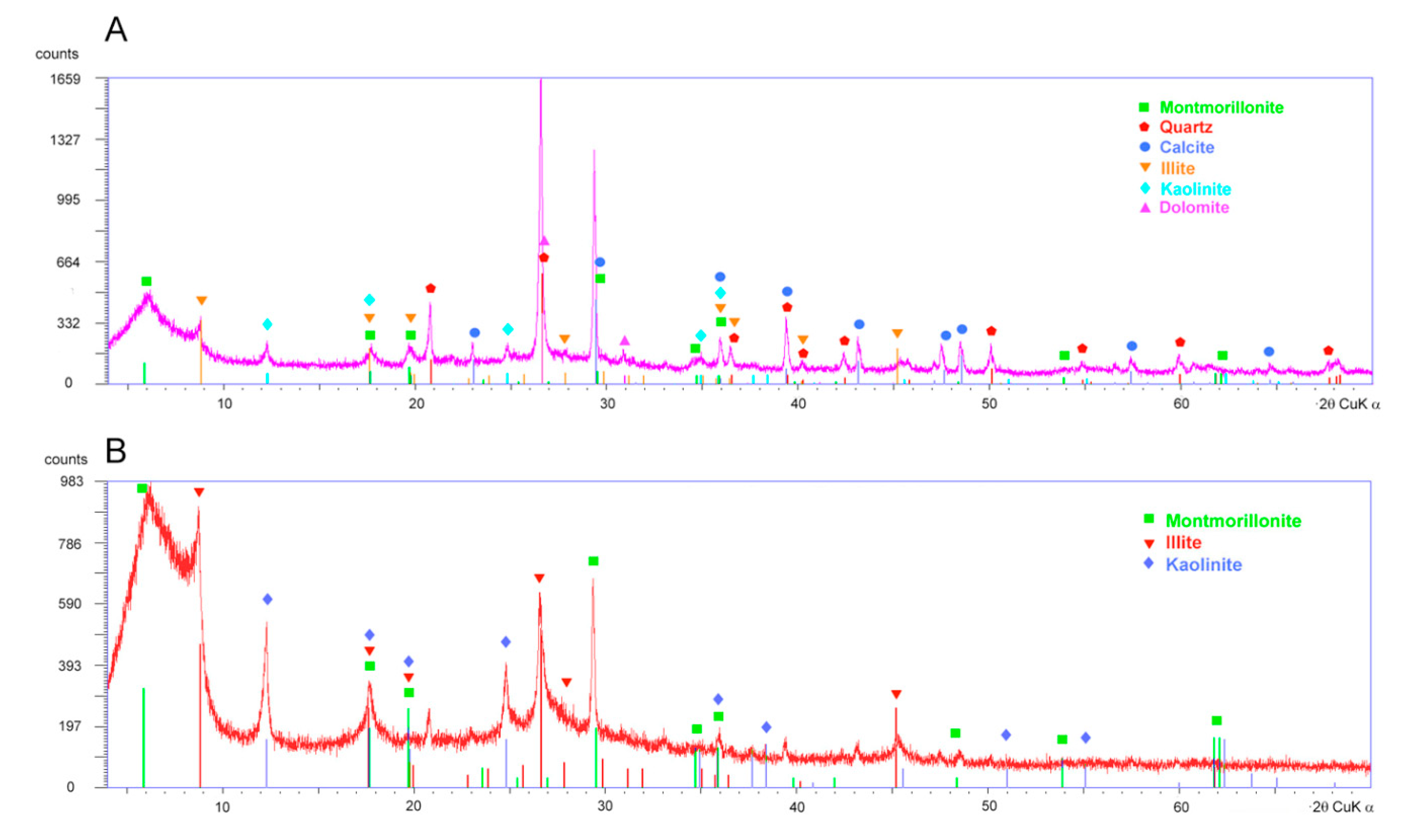
5.1. Mineralogical Characteristics of the Slip Zone

The XRF (X-ray fluorescence) results reveal that the slip zone contains high concentrations of SiO2, Al3+, K+, Mg2+, and Ca2+, as well as lower concentrations of Na+ (Table 2). This may indicate that the slip zone is rich in clay minerals.
From the XRD (X-ray diffractometry) diagrams, the main mineralogical associations were established. The powder sample diagram shows that the landslide-slip zone materials are mainly composed of quartz, clay minerals, calcite, and dolomite (Figure 5). Chlorite and micas (muscovite and paragonite) are also present in lesser proportions. The oriented sample (<2 μm fraction) diagrams show that the main clay minerals present in the slip zone are montmorillonite, illite, and kaolinite. The smectite content of the green layer located on the landslide slip surface is 38–46% [28]. The remaining mineral quantification was estimated by the Xpowder software [44] as follows: 8–15% kaolinite, 16–19% calcite, 10–14% mica, and 12–15% quartz.

5.2. Internal Geometry and Groundwater Flow in the Diezma Landslide

The ERT profiles carried out in the Diezma landslide show areas of high conductivity (with resistivity values of <20 Ωm) coinciding with the presence of saturated materials. The low resistivity values are linked to the nature of clayey materials and/or to a greater degree of moisture. The highest resistivity contrast can be found at the bottom of these zones, which corresponds with the failure plane of the landslide according to the available data obtained from the extensometers and inclinometers installed in several boreholes (see Figure 3). In addition, the ERT data indicate that the slip surface constitutes the wall of the colluvial aquifer; thus, the materials in this zone are completely saturated. These interpretations are based on the analysis of the mentioned boreholes carried out in the landslide during the investigation phase just after the failure (Figure 6). These boreholes show that most of the mobilized material (Figure 6a) is composed of clays of various colors and dispersed red blocks, pebbles, and large fragments (up to 40 cm in size) of sandstone and dolostone within their matrix. There are not great lithological differences in the stratigraphic column until we find the green clays layer coinciding to the failure plane. Therefore, we inferred that the observed variation in resistivity values is mainly due to the water content and not to differences in the lithology of the materials. Figure 7 shows the different electrical profiles that were carried out.
In the longitudinal profile (LP-1), the abrupt change in resistivity at the southern end of the profile is attributed more to a drying effect caused by the drainage borehole than to a variation in the clay composition. Thus, the resistivity values are strongly affected by the degree of soil moisture. The lowest resistivity values (below 10 Ω.m) belong to those materials that are close to the saturation state. The substrate of the Maláguide contact is located in the deepest part of the profile and has a value of 20 Ω.m. From this point on, there is a significant increase in the resistivity gradient. This contact is also revealed by the overlap of a ground-penetrating radar (GPR) section with the coincident resistive field, where the resistive gradient corresponds to the deep reflective layer (Figure 7).
In the intermediate profiles, the area with lower resistivity in the central sector should correspond to a channel where water circulated, thus indicating that its materials are saturated. In the last profile, TP-4, the resistivity gradient is located at the bottom of the profile, such that the isolines of 20 and 40 Ω.m are slightly separated. This information, when correlated with the borehole data, allows us to set the sliding level between these isolines.

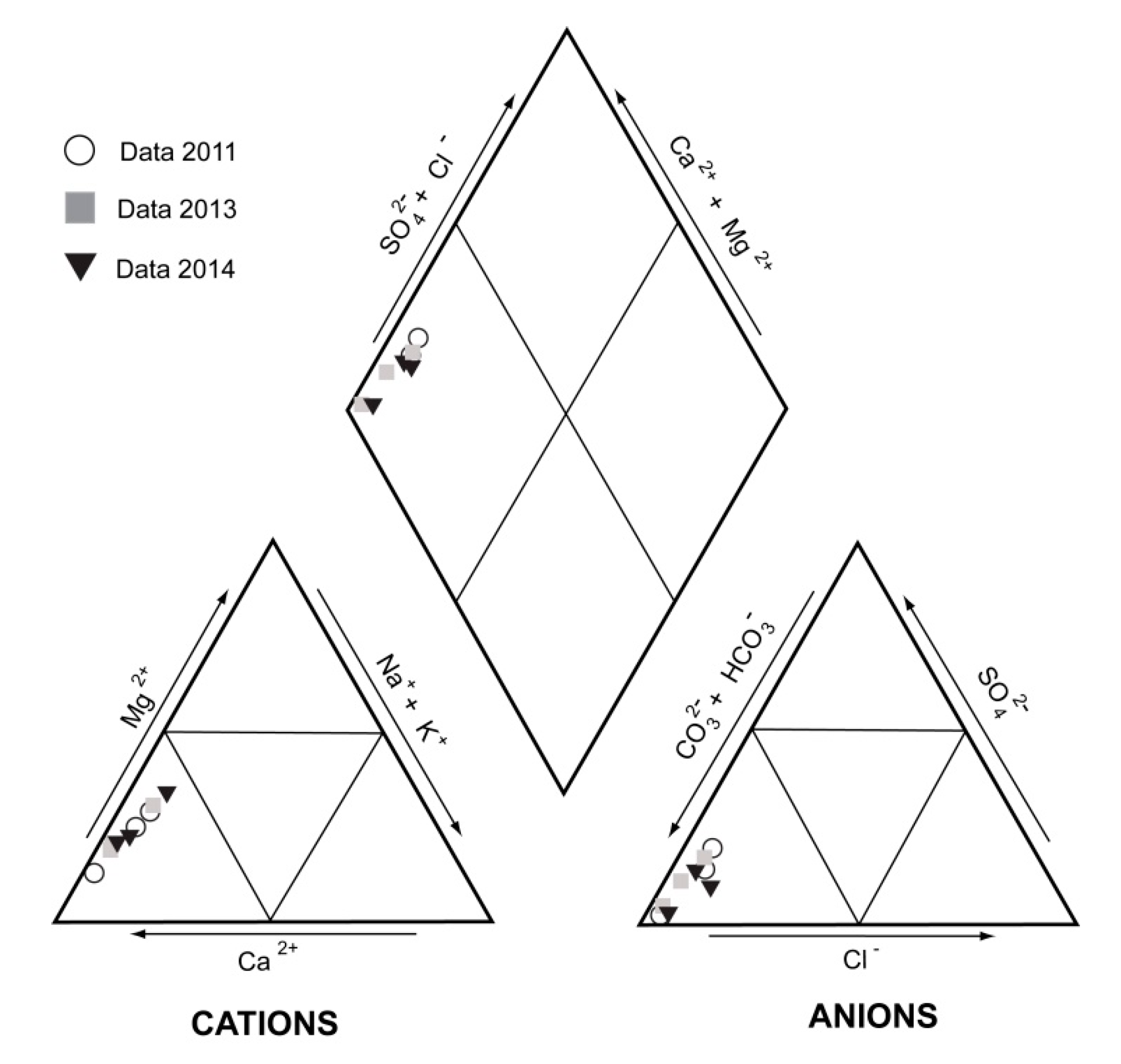
5.3. Groundwater Hydrochemistry in the Diezma Landslide

Water chemistry can be used as a tool to identify the processes and mechanisms affecting the groundwater (e.g., [48,49,50]). Therefore, the groundwater composition and mineralogy of the different rocks present in the area have been used to determine the source of the major ions in the water and their relations with weathering processes.
The groundwater in the landslide is generally Ca2+-HCO3 type (Table 3 and Figure 8), with Ca ranging from 1.51 to 2.53 mmol/L and HCO3 ranging from 3.39 to 5.95 mmol/L. In general, chemical analyses show increases in Ca2+, Mg2+, alkalinity, and total dissolved solids (TDS) as the water moves from points 1 to 3 (see Figure 3). Taking into account the mineralogy of the aquifer rocks, the concentrations of the dissolved major elements appear to be determined by the dissolution of carbonate minerals (e.g., calcite and dolomite), which contributes the observed Ca2+, Mg2+, and HCO3 to the water.
As mentioned above, ion–ion plots (see Figure 9) were used to infer the possible processes affecting the hydrogeochemical evolution of the studied waters (e.g., [51]). The values of Ca2+ + Mg2+ versus total cations (Figure 9a) lie along a 1:1 line, suggesting that Ca2+ and Mg2+ are the main cations present in the waters. When data deviate from that line, it indicates that other cations (Na+ and/or K+) contribute substantially to the water chemistry. The plot of Ca2+ + Mg2+ versus bicarbonate + sulfate (Figure 9b) shows that, in general, most of the points fall along the equiline, which indicates that the Ca2+ and Mg2+ chemistry is largely explained by carbonate and sulfate weathering processes. The points that fall on the Ca2+ and Mg2+ side indicate excess Ca and Mg derived from other processes, such as ion exchange reactions [48].
Waters derived from calcite or dolomite dissolution normally lie above the 2:1 line on the bicarbonate versus Ca plot and the bicarbonate versus Ca2+ + Mg2+ plot, respectively ([52,53]; Figure 9c,d). The results show that some of the samples lie above the 2:1 line, indicating that they originated from carbonate dissolution. However, there is a group of samples that do not fall above the 2:1 line, which suggests that Ca2+ and Mg2+ are involved in additional geochemical processes other than carbonate dissolution (e.g., ionic exchange processes). The Ca2+/Mg2+ ratios of the waters support the hypothesis of the dissolution of carbonates as a main process in the studied system (Figure 9e, Table 3). If the Ca2+/Mg2+ molar ratio is equal to one, the dissolution of dolomite should occur [54], whereas higher ratios, such as the ratios from our waters, are indicative of a greater calcite contribution. Previous researchers [55] also explained that a higher Ca2+/Mg2+ molar ratio (>2) is indicative of the dissolution of silicate minerals.
Finally, it is important to highlight the good 1:1 correlation between the molar dissolved concentrations of Na+ and Cl in most of the studied waters (Figure 9f), suggesting that halite dissolution is the main source of Na+ and Cl in the system [50]. Those values that deviate from the 1:1 line indicate that the Na concentration is involved in ion exchange processes and that Na+ and Cl concentrations do not increase simultaneously.
Saturation indices are also useful for evaluating and supporting the processes deduced from ion–ion plots. Then, the saturation indices of the main minerals controlling the water chemistry can be calculated using PHREEQC (Table 3). The saturation index (SI) indicates whether a solution is in equilibrium (SI = 0), undersaturated (<0), or oversaturated (>0) with respect to a solid phase. In practice, equilibrium can be assumed to span a range of −0.05 to +0.05 [56]. If water is undersaturated with respect to a given mineral, then that mineral would dissolve if it were present in the system. However, supersaturation is not equivalent to precipitation. If precipitation kinetics is slow, solutions can remain supersaturated and not precipitate with regard to a mineral phase for a long time [56].
The results of the calculated saturation indices (Table 3) revealed that the waters are undersaturated with respect to halite, gypsum, and anhydrite and are close to equilibrium or slightly oversaturated with respect to calcite and dolomite. This indicates that halite and gypsum (or anhydrite) will dissolve, which is consistent with the results of the ion-ion plots (Figure 9b,f). The obtained values for calcite and dolomite, together with the results of the ion–ion plots, suggest that they could be dissolved. However, dolomite dissolves much more slowly than calcite [57,58,59]; therefore, its dissolution is less plausible.
Another tool used to test the hydrochemical evolution of groundwater is stability diagrams, which can be used to help define the reactions that control water chemistry. However, especially in clays, there are some sources of uncertainty in setting the boundaries between these phases in stability diagrams (e.g., experimental measurements, inconsistencies introduced from standard free-energies, and differences in the properties of the mineral phases [60]). Therefore, we constructed a diagram using different equilibrium constants obtained from the literature for the following reaction:
6 Ca-Montmorillonite + 2 H+ + 23 H2O = 7 Kaolinite + Ca2+ + 8 H4SiO4
The values used here are log K = −15.7, log K = −18.4 ± 0.8 and log K = −16.3 ± 1, which correspond to those proposed by [61,62,63], respectively. The results (Figure 10) show that when considering the uncertainties of the constants and the different reported values, the three samples plot very close to the equilibrium line, suggesting that one mineral is dissolving incongruently and resulting in the formation of the other.

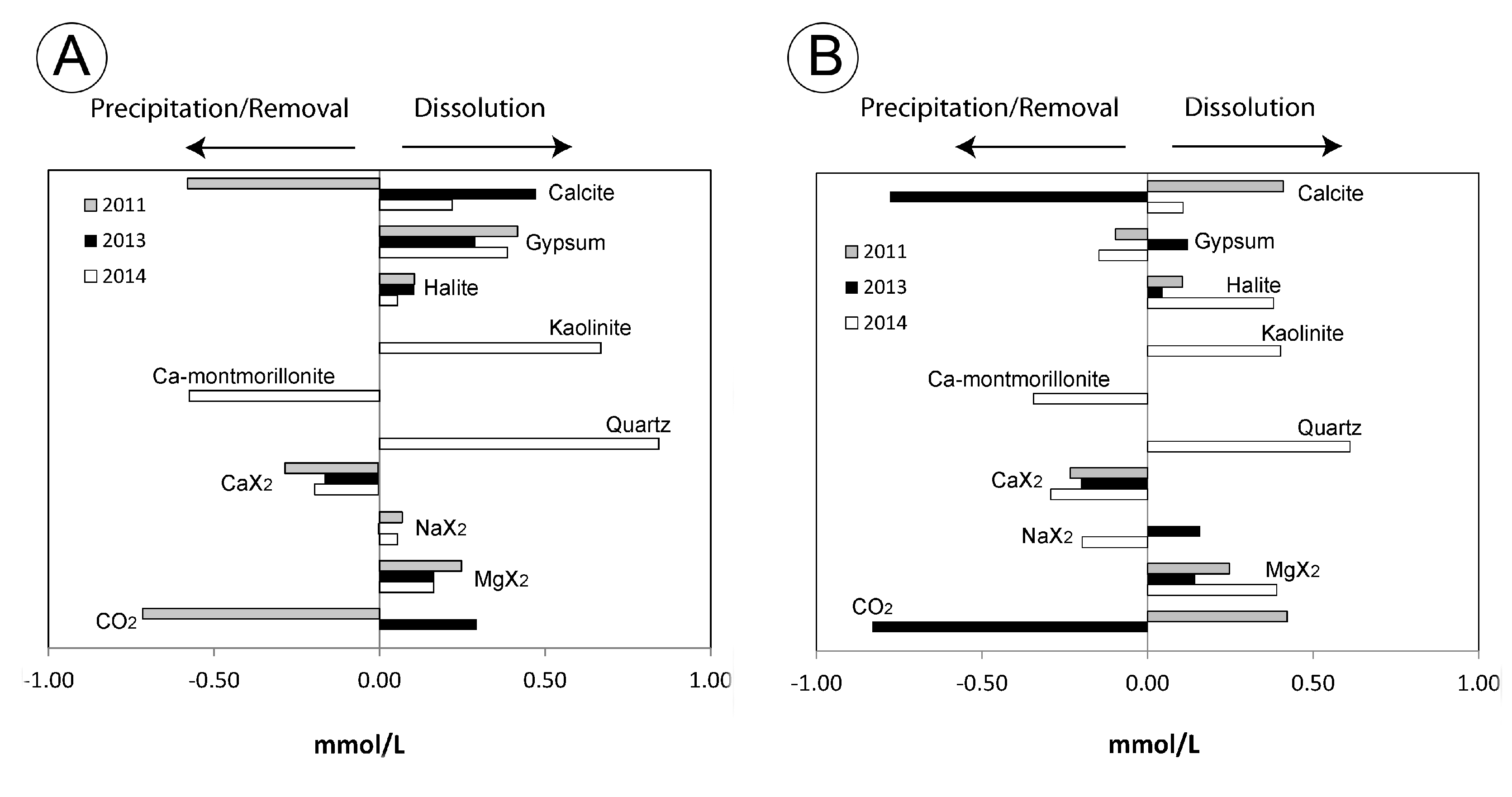
5.4. Process Quantification by Mass-Balance Calculations

The analyses of the hydrochemical trends for the main elements of the system, together with speciation-solubility calculations and the stability diagram of the clays, allow us to deduce the general geochemical processes that could control the composition of the water. Therefore, based on the chemical data and field mineralogical observations, it is proposed that the main geochemical processes are the dissolution or precipitation of calcite, halite, gypsum, quartz, kaolinite, and Ca-montmorillonite, as well as cationic exchange reactions. Mass-balance and reaction-path simulations were carried out to quantify the relative importance of those processes along the flow path (i.e., from point 1 to point 2 and from point 2 to point 3).
Mass-balance models, used in geochemistry to evaluate the chemical transfers between phases in water (e.g., [51,64,65,66]), are based on the principle that if one water evolved from another, the compositional differences can be accounted for by the minerals and gases that leave or enter that packet of water [67] within specified compositional uncertainty limits:
initial water + reactants → final water + products
An uncertainty limit of 0.05 (5%) was adjusted for all of the analytical data used in our modelling calculations, and then PHREEQC considers these uncertainties analyses to solve alkalinity-balance and element concentration-balance. These models are not unique; therefore, they were constrained based on the bulk mineralogical composition of the soil and the hydrogeochemical trends observed in the system. The plausible phases included in the model are calcite, gypsum, halite, kaolinite, Ca-montmorillonite, quartz, CO2, and CaX2, NaX, and MgX2 species for ionic exchange reactions of Ca or Mg for Na on exchange sites. For those plausible phases, the chemical evolution of the water along the water path is constrained by relationships of conservation of mass. The equations to calculate the mass transfer coefficients (αphase) are the following:
∆ mT, Ca = αcalcite + αgypsum + αCa-montmorillonite + αCa-exchange
∆ mT, Na = αhalite + αNa-exchange
∆ mT, C = αcalcite + αCO2
∆ mT, SO42− = αgypsum
∆ mT, Cl = αhalite
∆ mT, Mg = αMg-exchange
∆ mT, SiO2 = αquartz + αkaolinite + αCa-montmorillonite
where ∆ mT are the change in total moles of an element in solution along the flow path (final water minus initial water).
The summary of the best modelling results obtained here is shown in Figure 11. The mass-balance results suggest that geochemical processes involving carbonates, gypsum, halite, kaolinite, quartz, and Ca-montmorillonite, as well as ion exchange reactions, control the water chemistry; this is consistent with the results of the ion-ion analysis and the observed chemical trends.
The rainfall occurring in the months close to the sampling could have some influence on the dissolution and/or precipitation of different mineral phases. The first water sampling was carried out in October 2011, the second sampling was performed in February 2013, and the final sampling was performed in November 2014. Some differences in terms of recorded rainfall are observed between these three years. We collected pluviometric data from the nearest measurement station to analyze the amount of precipitation recorded in the three months before each sampling (Figure 12).
Thus, it can be observed that the first sampling year was the driest; only precipitation during the month of sampling is registered. However, the accumulated precipitation is quite high in almost all of the months prior to the second sampling. Finally, in 2014, the cumulative precipitation increases gradually, with a value of zero in the third month prior to sampling and high values (<100) observed during the month of sampling.
The models indicate that the processes of the precipitation and dissolution of calcite alternate based on the humidity of a given year. We observed the precipitation of calcite between points 1 and 2 and the dissolution of calcite between points 2 and 3 in the driest year (2011). The opposite trends occurred during the wetter year (2013). During the intermediate year (2014), we observed the dissolution of calcite along the groundwater path. Considering that the study area has a semi-arid climate, the conditions of the 2011 sampling period are the most typical, which may explain the existence of calcite precipitates associated with the clay-bearing layer observed in the upper part of the landslide (between points 1 and 2). This mineral association is also observed in moonmilks of Carlsbad Caverns and other caves of Guadalupe Mountains [68]. Nevertheless, the setting is very different and special with respect to our case study. The dissolution processes inferred from the 2011 and 2014 samples between points 2 and 3 explain why no calcite precipitates associated with the slip zone are observed in the toe of the landslide.

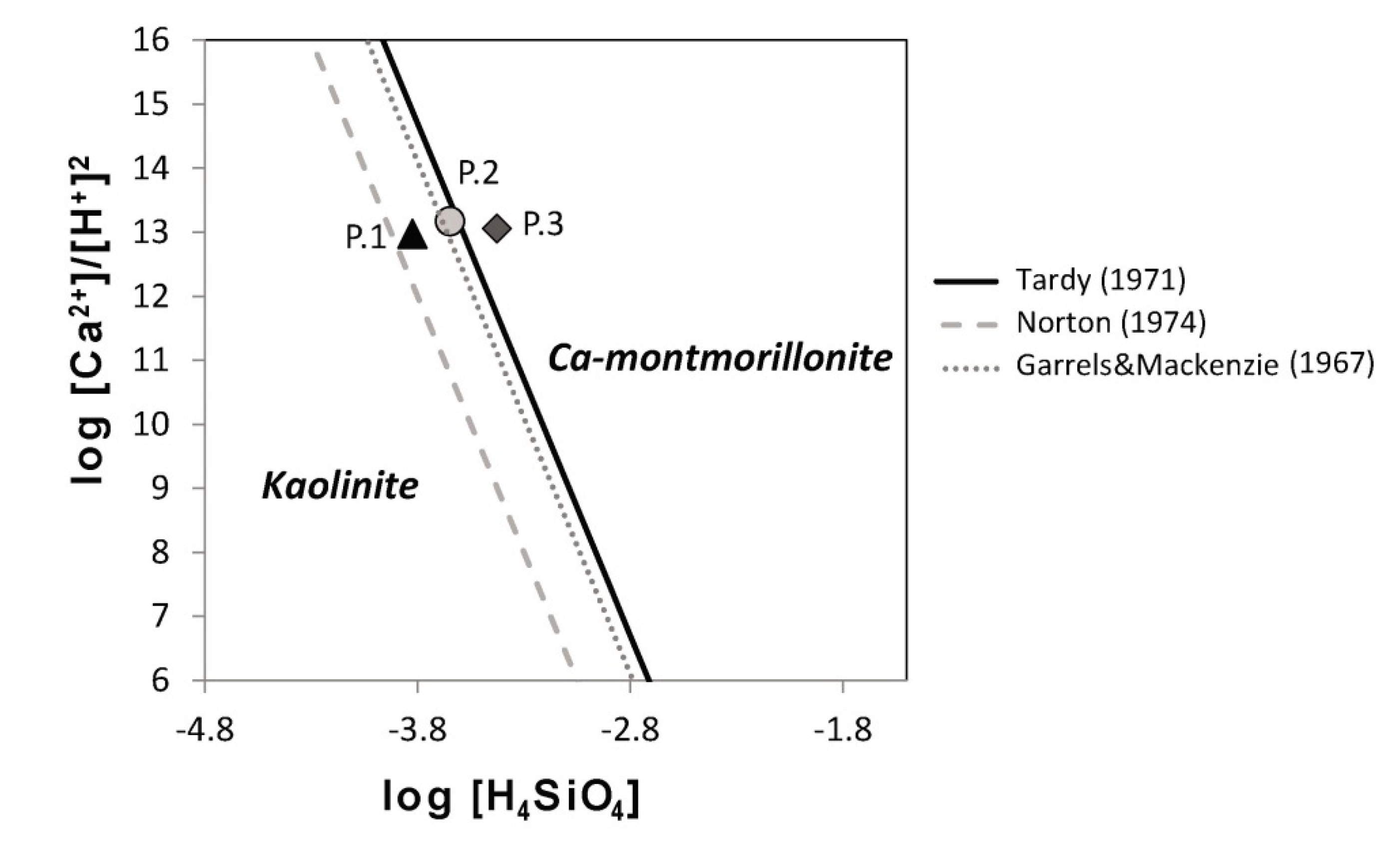
5.5. Direct modelling: Reaction-Path Calculations

Inverse modelling calculations have indicated that the evolution of these waters is mainly controlled by the dissolution-precipitation of calcite, halite, gypsum, kaolinite, quartz, and Ca-montmorillonite, as well as ionic exchange reactions. Mass-balance approaches do not provide or justify unequivocal interpretations of the geochemical processes controlling the hydrochemical evolutions of these waters. Therefore, reaction-path calculations were carried out to use a direct model to assess the feasibility of the conceptual model proposed for the studied waters.
With this objective, the waters from points 1 to 2 and from points 2 to 3 were reacted with the amounts of dissolved or precipitated phases obtained in the mass-balance calculations. A comparison of the measured concentrations of the main ions to those calculated from the model is shown in Table 4. As displayed in Table 4, the calculated compositions of the solutions after the precipitation-dissolution and ionic exchange processes considered in the conceptual model and those of the waters are the same within 5% uncertainty. The good agreement between the inverse model and reaction path calculations observed here provide evidence that the processes considered here are qualitatively and quantitatively suitable to describe the geochemical evolution of the waters along the studied pathway.

6. Discussion

6.1. Where Does the Clay-Bearing Layer of the Diezma Landslide Come From?

The speciation-solubility, reaction-path, and mass-balance calculations performed here allowed us to identify the main geochemical processes occurring in the waters along the flow-path (i.e., from point 1 to point 3), which are the dissolution-precipitation of calcite and gypsum, the dissolution of halite and kaolinite, the precipitation of Ca-montmorillonite, and ionic exchange processes. These processes modify the water composition, favoring the formation of Ca-montmorillonite (smectites), as detected by XRD (Figure 5). Previous studies have noted the presence of high concentrations of Ca and HCO3 in the groundwater along the slip surface and the fact that they increase from the head to the toe of landslides [1,69]. The dissolution of calcite leads to increases in the concentrations of calcium and bicarbonate in waters:
CaCO3 + CO2 + H2O = Ca2+ + 2HCO3
In the presence of CO2, Ca2+ and HCO3, the equilibrium equation between Ca-montmorillonite and kaolinite could be expressed as follows [1]:
6 Ca-Montmorillonite + 2 CO2 = 7 Kaolinite + Ca2+ + 2 HCO3 + 8 SiO2 + 9H2
Therefore, the increases in calcium and bicarbonate due to calcite dissolution should favor the formation of Ca-montmorillonite (smectite). For example, previous researchers [1] observed an excellent correlation between the concentrations of these anions and the amount of montmorillonite in the slip zone, which increased toward the lower parts of the landslide. Furthermore, the previous work also indicated that the formation of smectite required groundwater with an HCO3 concentration of higher than 40 mg/L in the slip surface of Tertiary volcanic rocks in Japan. Therefore, the chemical composition of water plays a major role in determining the type of clay mineral that is formed.
Our mass-balance calculations support the incongruent dissolution of kaolinite and the formation of Ca-montmorillonite along the flow path. Furthermore, the compositions of the three points plot close to the equilibrium line in the kaolinite-Ca-montmorillonite stability diagram (Figure 10), which suggests that one of the mineral phases is dissolving and that the other is precipitating. The inverse modelling results show that the incongruent dissolution of kaolinite results in the formation of Ca-montmorillonite. These results are in good agreement with the mineralogical composition observed in the Diezma landslide, where there is a smectite concentration (montmorillonite-beidellite) present in the shear surfaces. This mineral transformation, which is triggered by calcite dissolution, represents one of the factors that conditioned the failure and current instability in the Diezma landslide.
However, why did Shuzui [1] observe that the concentration of clay minerals, and hence the mineral transformation, increased in the slip surface? It is possible to hypothesize that the origin of the observed high concentration of smectite clays in slip surfaces seems to be linked to the enhancement of chemical reactions due to the highly reactive surface areas in failure planes where layers with small particles are formed. This reasoning is inspired by the published results of laboratory tests simulating the processes occurring in slip surfaces and specific studies focusing on mineral formation in fault zones: (1) Laboratory tests using ring shear apparatuses show that the reordering of particles by grain size occurs in landslide shear zones, thus creating layers with small particles parallel to the slip surface [70]. Moreover, fine particles were also added to the shear zone by mechanical crushing during the process of shearing [71]. This process could be fed back by mineralogical transformation. (2) The study of the formation of new minerals caused by fluid–rock interactions in fault zones, which may be considered analogous examples of landslide slip surfaces because tectonic faults are governed by frictional sliding and behave similarly to them, shows that the presence of some minerals, such as quartz, increases the permeability of fault gouge materials, allows for the circulation of water through the fault zone, and leads to the strong leaching of the protolith and the crystallization of new authigenic minerals (illite, kaolinite, smectite, and gypsum) [72]. In the case of the Diezma landslide, although the climate in the region is semi-arid, there is always a flow of water present in the studied slope. The carbonate karstic aquifer located in the upper part of the hillside feeds the colluvial material of the slope, and, as our geophysical data indicate, the colluvium channels the groundwater flow in the slope, probably because of its higher permeability, thus enhancing the geochemical reactions described above.

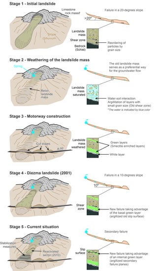
6.2. Conceptual Model Proposed for the Evolution of the Diezma Landslide

Considering all of the information presented and discussed in the paper, we propose a conceptual model of the evolution of the Diezma landslide (see Figure 13) by taking into account the information provided by our hydrogeochemical and geophysical study and those provided by previous studies. The main information to bear in mind is:
-
The Diezma landslide mobilized surficial deposit most likely produced by a former mass movement (see Section 3).
-
Clay-bearing layers enriched with smectite appear associated to slip surfaces (see Section 3).
-
Smectite are high-plasticity clays that give the materials very low residual friction angles (ϕr = 7°). This allows occurrence of landslides showing failure planes with very low inclination (<20 °) (see Section 3).
-
Bi-carbonate type waters infiltrated in the slope of Diezma landslide favored the transformation of kaolinite to smectite (see Section 5).
-
Old slip surfaces may represent preferential flow ways for groundwater (see Section 6.1).
-
Chemical reactions in slip surfaces can be enhanced because they are composed of fine particles (i.e., layers with highly reactive surface areas) (see Section 6.1).
Therefore, we infer that the Diezma landslide mobilized the material of a relict landslide that dragged flysch-like and carbonate rocks in its movement along a ca. 20-degree paleo-slope (Stage 1). We consider that the pre-existing slip surface of the mentioned relict landslide was the origin of the studied clay-bearing layers. The mineral transformations could have been enriched these slip surfaces with an anomalously high concentration of smectite. This process would have been controlled by (1) the bicarbonate-type waters that feed the groundwater of the slide mass and (2) the enhancement of chemical reactions in the relict landslide shear zones (i.e., layers with fine particles) (Stage 2).
In 2001, the main failure of the Diezma landslide occurred. This took place mainly because the cut-slope excavated during the construction of the A-92 motorway was not properly stabilized. The clay-bearing layer was neither detected nor considered, and engineering structural measures were not applied because the stability analyses of this cut-slope only took into account the mechanical properties of the outcropping material (Stage 3). As a result, a landslide was triggered that mobilized much of the hillside along a ca. 10-degree failure plane by taking advantage of the main clay-bearing layer (Stage 4). In 2010, a partial sector of the landslide body was reactivated over other argillized secondary failure plane (Stage 5).

7. Conclusions

This research highlights the useful output that can provide hydrogeochemical analyses in landslide investigations. The geochemical characterization of the groundwater and the quantification of its geochemical processes are essential tools to understand the evolution and current behavior of unstable slopes. In the presented case study, we form a hypothesis about the history of the Diezma landslide that incorporates something not yet taken into account; that is, how the water–soil interaction processes created the conditions that led to this slope failure. In this sense, we strongly believe that the processes described here are responsible for the occurrence and evolution of many damaging landslides observed in places where groundwater from karstic aquifers (i.e., bi-carbonate type water) interact with marly-clayey soils. This have important implications in slope stability analyses because, as happened in Diezma landslide, the stability of a slope may be determined by a very thin layer of high-plasticity clays formed along internal discontinuities of the slope materials and not observed in the surface, and therefore not considered in the slope stability calculations. Thus, our work indicates, in addition to an explanation for the secondary high-plasticity clay layers formation, a particular geological setting where engineers should be more cautious in their slope investigations due to the possibility of finding these types of layers. For example, the proposed hypothesis could explain the mechanisms of slope destabilization in comparable geological settings as the Three Gorge Reservoir region (China). Nevertheless, further research focused on lab experiments and studies in other similar landslides is needed to verify our hypothesis. The presented results and argumentation may be the starting point to open a fruitful line of research related to the application of hydrogeochemical studies in landslide investigation.

Author Contributions

Conceptualization, J.C., M.P.A., J.P.G., and J.M.A.; methodology, J.C., M.P.A., J.P.G., and J.M.A.; software, J.C., M.P.A., J.P.G., and J.M.A.; validation, J.C., M.P.A., J.P.G., and J.M.A.; formal analysis, J.C., M.P.A., and J.P.G.; investigation, J.C., M.P.A., J.P.G., and J.M.A; resources, M.P.A., J.P.G., and J.M.A; data curation, J.C. and J.M.A.; writing—original draft preparation, J.C.; writing—review and editing, M.P.A., J.P.G., and J.M.A.; supervision, M.P.A., J.P.G., and J.M.A.; project administration, J.M.A.; funding acquisition, J.M.A. All authors have read and agreed to the published version of the manuscript.

Funding

This study was supported by the research projects PID2019-107138RB-I00 funded by the Spanish Ministry of Science and Innovation and P18-RT-3632 funded by the Junta de Andalucía.

Acknowledgments

We are grateful to the two reviewers and Enrico Conte for their constructive comments.

Conflicts of Interest

The authors declare no conflict of interest.

References

  1. Shuzui, H. Process of slip surface development and formation of slip surface clay in landslide in Tertiary volcanic rocks, Japan. Eng. Geol. 2001, 61, 199–219. [Google Scholar] [CrossRef]
  2. Anson, R.; Hawkins, A. Movement of the Soper’s Wood landslide on the Jurassic Fuller’s Earth, Bath, England. Bull Eng. Geol. Environ. 2002, 61, 325–345. [Google Scholar] [CrossRef]
  3. Conte, E.; Donato, A.; Pugliese, L.; Troncone, A. Analysis of the Maierato landslide (Calabria, Southern Italy). Landslides 2018, 15, 1935–1950. [Google Scholar] [CrossRef]
  4. Conte, E.; Pugliese, L.; Troncone, A. Post-failure analysis of the Maierato landslide using the material point method. Eng. Geol. 2020, 277. [Google Scholar] [CrossRef]
  5. Bogaard, T.; Guglielmi, Y.; Marc, V.; Emblanch, C.; Bertrand, C.; Mudry, J. Hydrogeochemistry in landslide research: A review. Bull. Société Géologique Fr. 2007, 178, 113–126. [Google Scholar] [CrossRef]
  6. L’Heureux, J.S.; Locat, A.; Leroueil, S.; Demers, D.; Locat, J. Landslides in Sensitive Clays. In Geoscience to Risk Management; Springer: Dordrecht, The Netherlands, 2014; p. 418. [Google Scholar]
  7. Di Maio, C.; Santoli, L.; Schiavone, P. Volume change behaviour of clays: The influence of mineral composition, pore fluid composition and stress state. Mech. Mater. 2004, 36, 435–445. [Google Scholar] [CrossRef]
  8. Alvarado, G.; Vega, E.; Chaves, J.; Vászquez, M. Los grandes deslizamientos (volcánicos y no volcánicos) tipo debris avalanche en Costa Rica. Rev. Geol. Amér. Cent. 2004, 30, 83–99. [Google Scholar] [CrossRef] [Green Version]
  9. Waythomas, C.F.; Pierson, T.C.; Major, J.J.; Scott, W.E. Voluminous ice-rich and water-rich lahars generated during the 2009 eruption of Redoubt Volcano, Alaska. J. Volcanol. Geotherm. Res. 2013, 259, 389–413. [Google Scholar] [CrossRef]
  10. Ferrer, M.; Ayala-Carcedo, F. Landslides in Spain: Extent and Assessment of the Climatic Susceptibility. In Proceedings of the Symposium on Engineering Geology and the Environment Balkema, Rotterdam, The Netherlands, 23–27 June 1997; Marinos, P.G., Koukis, G.C., Tsiambaos, G.C., Stournaras, G.C., Eds.; pp. 625–631. [Google Scholar]
  11. Azañón, J.M.; Azor, A.; Yesares, J.; Tsige, M.; Mateos, R.M.; Nieto, F.; Delgado, J.; López-Chicano, M.; Martín, W.; Rodríguez-Fernández, J. Regional-scale high-plasticity clay-bearing formation as controlling factor on landslides in Southeast Spain. Geomorphology 2010, 120, 26–37. [Google Scholar] [CrossRef]
  12. Korup, O.; Clague, J.J.; Hermanns, R.L.; Hewitt, K.; Strom, A.L.; Weidinger, J.T. Giants landslides, topography, and erosion. Earth Planet. Sci. Lett. 2007, 261, 578–589. [Google Scholar] [CrossRef]
  13. Hancox, G.T. The 1979 Abbotsford Landslide, Dunedin, New Zealand; a retrospective look at its nature and causes. Landslides 2008, 5, 177–188. [Google Scholar] [CrossRef]
  14. Dahal, R.K.; Hasegawa, S.; Yamanaka, M.; Dhakal, S.; Bhandary, N.P.; Yatabe, R. Comparative analysis of contributing parameters for rainfall-triggered landslide in the Lesser Himalaya of Nepal. Env. Geol. 2009, 58, 567–586. [Google Scholar] [CrossRef]
  15. Lundström, M.; Larsson, R.; Dahlin, T. Mapping of quick clay formations using geotechnical and geophysical methods. Landslides 2009, 6, 1–15. [Google Scholar] [CrossRef] [Green Version]
  16. Van Den Eeckhaut, M.; Hervás, J.; Jaedicke, C.; Malet, J.P.; Montanarella, L.; Nadim, F. Statistical modelling of Europe-Wide landslide susceptibility using limited landslide inventory data. Landslides 2012, 9, 357–369. [Google Scholar] [CrossRef]
  17. Dang, K.; Sassa, K.; Fukuoka, H.; Sakai, N.; Sato, Y.; Takara, K.; Quang, L.H.; Duy-Loi, H.; Van-Tiem, P.; Duc-Ha, N. Mechanism of two rapid and long-runout landslides in the 16 April 2016 earthquake using a ring-shear apparatus and computer simulation (LS-RAPID). Landslides 2016, 13, 1525–1534. [Google Scholar] [CrossRef]
  18. Prior, B.D.; Ho, C. Coastal and mountain slope instability on the islands of St. Lucia and Barbados. Eng. Geol. 1972, 6, 1–18. [Google Scholar] [CrossRef]
  19. Egashira, K.; Gibo, S. Colloid-chemical and mineralogical differences of smectites take from argillized layers, both from within and outside the slip surfaces in the Kamenose landslide. Appl. Clay Sci. 1988, 3, 253–262. [Google Scholar] [CrossRef]
  20. Angeli, M.C.; Pasuto, A.; Silvano, S. Towards definition of slope instability behaviour in the Alverà mudslide (Cortina d’Ampezzo, Italy). Geomorphology 1999, 30, 201–211. [Google Scholar] [CrossRef]
  21. Wen, B.P.; Aydin, A.; Aydin, N.S. Geochemical characteristics of the slip zones in granitic saprolite and the implication in their origin and evolution. Environ. Geol. 2004, 47, 140–154. [Google Scholar] [CrossRef]
  22. Baoping, W.; Haiyang, C. Mineral Compositions and Elements Concentrations as Indicators for the Role of Groundwater in the Development of Landslide Slip Zones: A Case Study of Large-scale Landslides in the Three Gorges Area in China. Earth Sci. Front. 2007, 14, 98–106. [Google Scholar]
  23. Li, X.; Liao, Q.; Wang, S.; Liu, J.; Lee, S. On evaluating the stability of the Baiyian ancient landslide in the Three Gorges Reservoir area, Yangtze River: A geological history analysis. Environ. Geo. L 2008, 55, 1699–1711. [Google Scholar] [CrossRef]
  24. Tang, H.; Li, C.; Hu, X.; Su, A.; Wang, L.; Wu, Y.; Criss, R.; Xiong, C.; Li, Y. Evolution characteristics of the Huangtupo landslide based on in situ tunnelling and monitoring. Landslides 2015, 12, 511–521. [Google Scholar] [CrossRef]
  25. Jiang, J.; Xiang, W.; Rohn, J.; Zen, W.; Schleier, M. Research on water-rock (soil) interaction by dynamic tracing method for Huangtupo landslide, Three Gorges Reservoir, PR China. Environ. Earth. Sci. 2015, 74, 557–571. [Google Scholar] [CrossRef]
  26. Jian, W.; Wang, Z.; Yin, K. Mechanism of the Anlesi landslide in the Three Gorges Reservoir, China. Eng. Geol. 2009, 108, 86–95. [Google Scholar] [CrossRef]
  27. Xu, Q.; Liu, H.; Ran, J.; Li, W.; Sun, X. Field monitoring of groundwater responses to heavy rainfalls and the early warning of the Kualiangzi landslide in Sichuan Basin, southwestern China. Landslides 2016, 13, 1555–1570. [Google Scholar] [CrossRef]
  28. Nieto, F.; Abad, I.; Azañón, J.M. Smectite quantification in sediments and soils by thermogravimetric analyses. Appl. Clay Sci. 2008, 38, 288–296. [Google Scholar] [CrossRef]
  29. Guglielmi, Y.; Bertrand, C.; Compagnon, F.; Follacci, J.P.; Mudry, J. Acquisition of water chemistry in a mobile fissured basement massif: Its role in the hydrogeological knowledge of the La Clapière landslide (Mercantour massif, southern Alps, France). J. Hydrol. 2000, 229, 138–148. [Google Scholar] [CrossRef]
  30. De Montety, V.; Marc, V.; Emblanch, C.; Malet, J.P.; Bertrand, C.; Maquaire, O.; Bogaard, T.A. Identifying the origin of groundwater and flow processes in complex landslides affecting black marls: Insights from a hydrochemical survey. Earth Surf. Process. Landf. 2007, 32, 32–48. [Google Scholar] [CrossRef]
  31. Cervi, F.; Ronchetti, F.; Martinelli, G.; Bogaard, T.A.; Corsini, A. Origin and assessment of deep groundwater inflow in the Ca’ Lita landslide using hydrochemistry and in situ monitoring. Hydrol. Earth Syst. Sci. 2012, 16, 4205–4221. [Google Scholar] [CrossRef] [Green Version]
  32. Rodríguez-Peces, M.J.; Azañón, J.M.; García-Mayordomo, J.; Yesares, J.; Troncoso, E.; Tsige, M. The Diezma landslide (A-92 motorway, Southern Spain): History and potential for future reactivation. Bull. Eng. Geol. Environ. 2011, 70, 681–689. [Google Scholar] [CrossRef]
  33. Delgado, J.; Garrido, J.; Lenti, L.; Lopez-Casado, C.; Martino, S.; Sierra, F.J. Unconventional pseudostatic stability analysis of the Diezma landslide (Granada, Spain) based on a high-resolution engineering-geological model. Eng. Geol. 2015, 184, 81–95. [Google Scholar] [CrossRef] [Green Version]
  34. Bourgois, J.; Chauve, P.; Didon, J. La formation d’argiles a blocs dans la province de Cadix, Cordilleras Betiques, Espagne. Reun. Annu. Sci. Terre 1974, 2, 79. [Google Scholar]
  35. García-Dueñas, V.; Navarro-Vilá, F. Mapa Geológico de España E. 1:50.000, La Peza; I.G.M.E.: Madrid, Spain, 1980. [Google Scholar]
  36. Diputación Provincial de Granada e Instituto Tecnologico Geominero de España. Atlas Hidrogeológico de la Provincia de Granada; Diputación de Granada e ITGE: Granada, Spain, 1990; p. 107. [Google Scholar]
  37. Oteo-Mazo, C. Informe Sobre el Deslizamiento de Diezma (A-92) y las Soluciones para Estabilizarlo; Consejería de Obras Públicas y Urbanismo de la Junta de Andalucía: Madrid, Spain, 2001; p. 60. [Google Scholar]
  38. Delgado, J.; Garrido, J.; Lopez-Casado, C.; Lenti, L.; Martino, S.; Sierra, F.J. Diezma Landslide (Southern Spain): Geological Model and Seismic Response. Eng. Geol. Soc. Territ. 2015, 5. [Google Scholar] [CrossRef]
  39. Yesares-García, J.; Arocha, J.; Azañón, J.M.; Azor, A.; Díaz-Losada, E.; López-Chicano, M.; Martin, W.; Nieto, F.; Rodríguez-Fernández, J.; Garrido-Manrique, J. Factores Condicionantes en el Deslizamiento de Diezma (Granada, España). In Riesgos Naturales y Antropicos en Geomorfologia (Actas de la VIII Reunion Nacional de Geomorfologia); Benito, G., Díez-Herrero, A., Eds.; SEG y CSIG: Madrid, Spain, 2004; pp. 445–450. [Google Scholar]
  40. Oteo-Mazo, C. Diseño y ejecución del tratamiento para estabilizar el deslizamiento de Diezma (Granada). Spec. Vol. Congr. Andal. Carret. 2003, 3, 40–52. [Google Scholar]
  41. Azañón, J.M.; Azor, A.; Cardenal-Escarcena, J.F.; Delgado-García, J.; Delgado-Marchal, J.; Gómez-Molina, A.; López-Chicano, M.; López-Sánchez, J.M.; Mallorquí-Franquet, J.J.; Martín, W.; et al. Estudio Sobre la Predicción y Mitigación de Movimientos de Ladera en Vías de Comunicación Estratégicas de la Junta de Andalucía. Informe Final; Instituto Andaluz de Ciencias de la Tierra: Granada, Spain, 2006; p. 380. [Google Scholar]
  42. Azañón, J.M.; Abellán, A.; García, J.P.; Mateos, R.; Roldán, F.; Peña, J.P.; Galve, J.P.; Notti, D.; Monserrat, O.; Jover, R.T.; et al. Uso de Datos LIDAR Aéreos en 3D para el Control de Movimientos de Ladera. Caso de Estudio del Deslizamiento de Diezma (Granada). In Teledetección: Humedales y Espacios Protegidos. XVI Congreso de la Asociación Española de Teledetección; Bustamante, J., Díaz-Delgado, R., Aragonés, D., Afán, I., García, D., Eds.; Asociación Española de Teledetección: Sevilla, Spain, 2015; pp. 407–410. [Google Scholar]
  43. Umar, M.; Kassim, K.A.; Ping Chiet, K.T. Biological process of soil improvement in civil engineering: A review. J. Rock Mech. Geotech. Eng. 2016, 8, 767–774. [Google Scholar] [CrossRef] [Green Version]
  44. Martín-Ramos, J.D. Using XPowder: A Software Package for Powder X-Ray Diffraction Analysis; 2004; GR 1001/04; ISBN 84-609-1497-6, Spain. Available online: http://www.xpowder.com (accessed on 18 September 2020).
  45. Azañón, J.M.; Peña, J.A.; Teixidó, T.; Mateos, R.M.; Yesares, J.; Delgado, J.; Tsiege, M. Evaluación de la eficacia de los sistemas de drenaje mediante tomografía eléctrica en el deslizamiento de Diezma (Granada). In Proceedings of the VII Simposio Nacional sobre Taludes y Laderas Inestables, Barcelona, Spain, 27–30 October 2009. [Google Scholar]
  46. Parkhurst, D.L.; Appelo, C.A.J. Techniques and Methods. In Description of Input and Examples for PHREEQC Version 3. A Computer Program for Speciation, Batch-Reaction, One-Dimensional Transport, and Inverse Geochemical Calculations; U.S. Geological Survey: Denver, CO, USA, 2013; Book 6, Chapter A43. [Google Scholar]
  47. Ball, J.W.; Nordstrom, D.K. WATEQ4F User’s Manual with Revised Thermodynamic Data Base and Test Cases for Calculating Speciation of Major, Trace and Redox Elements in Natural Waters; Open-File Report 90 129; U.S. Geological Survey: Reston, VA, USA, 2001.
  48. Subramani, T.; Rajmohan, N.; Elango, L. Groundwater geochemistry and identification of hydrogeochemical processes in a hard rock region, Southern India. Environ. Monit. Assess. 2010, 162, 123–137. [Google Scholar] [CrossRef]
  49. Barberá, J.A.; Andreo, B.; Almeida, C. Using non-conservative tracers to characterise karstification processes in the Merinos-Colorado-Carrasco carbonate aquifer system (southern Spain). Environ. Earth. Sci. 2014, 71, 585–599. [Google Scholar] [CrossRef]
  50. Acero, P.; Gutiérrez, F.; Galve, J.P.; Auqué, L.F.; Carbonel, D.; Gimeno, M.J.; Gómez, J.B.; Asta, M.P.; Yechieli, Y. Hydrogeochemical characterization of an evaporite karst area affected by sinkholes (Ebro Valley, NE Spain). Geol. Acta 2013, 11, 389–407. [Google Scholar]
  51. Ledesma-Ruiz, R.; Pastén-Zapata, E.; Parra, R.; Harter, T.; Mahlknecht, J. Investigation of the geochemical evolution of groundwater under agricultural land: A case study in northeastern Mexico. J. Hydrol. 2015, 521, 410–423. [Google Scholar] [CrossRef] [Green Version]
  52. Garrels, R.M.; Mackenzie, F.T. Evolution of Sedimentary Rocks; W. W. Norton & Co.: New York, NY, USA, 1971; p. 397. [Google Scholar] [CrossRef]
  53. Holland, H.D. The Chemistry of the Atmosphere and Ocean; Wiley: New York, NY, USA, 1978; p. 351. [Google Scholar]
  54. Mayo, A.L.; Loucks, M.D. Solute and isotopic geochemistry and groundwater flow in the Central Wasatch-Range, Utah. J. Hydrol. 1995, 172, 31–59. [Google Scholar] [CrossRef]
  55. Katz, B.G.; Gopalan, T.B.; Bullen, T.D.; Davis, J.H. Use of chemical and isotopic tracers to characterize the interaction between groundwater and surface water in mantled Karst. Groundw. J. 1998, 35, 1014–1028. [Google Scholar] [CrossRef]
  56. Merkel, B.J.; Planer-Friedrich, B.; Nordstrom, D.K. Groundwater Geochemistry—A Practical Guide to Modeling of Natural and Contaminated Aquatic Systems; Springer: Berlin/Heidelberg, Germany, 2005; p. 200. [Google Scholar]
  57. Herman, J.S.; White, W.B. Dissolution kinetics of dolomite. Effects of lithology and fluid flow velocity. Geochim. Cosmochim. Acta 1985, 49, 2017–2026. [Google Scholar] [CrossRef]
  58. Langmuir, D. Aqueous Environmental Geochemistry; Prentice-Hall: Upper Saddle River, NJ, USA, 1997. [Google Scholar]
  59. Liu, Z.; Yuan, D.; Dreybrot, W. Comparative study of dissolution rate determinating mechanisms of limestone and dolomite. Environ. Geol. 2005, 49, 274–279. [Google Scholar] [CrossRef]
  60. Drever, J.I. The Geochemistry of Natural Waters; Prentice-Hall, Inc.: Englewood Cliffs, NJ, USA, 1982; p. 388. [Google Scholar] [CrossRef]
  61. Tardy, Y. Characterization of the Principal Weathering Types by the Geochemistry of Waters from Some European and African Crystalline Massifs. Chem. Geol. 1971, 7, 253–271. [Google Scholar] [CrossRef]
  62. Norton, D. Chemical mass transfer in the Rio Tanama system, west-central Puerto Rico. Geochim. Cosmochim. Acta 1974, 38, 267–277. [Google Scholar] [CrossRef]
  63. Garrels, R.M.; Mackenzie, F.T. Origin of the Chemical Composition of Some Springs and Systems. In Equilibrium Concepts in Natural Water Systems; American Chemical Society: Washington, DC, USA, 1967; Volume 67, pp. 222–242. [Google Scholar]
  64. Auqué, L.F.; Acero, P.; Gimeno, M.J.; Gómez, J.B.; Asta, M.P. Hydrogeochemical modeling of a thermal system and lessons learned for CO2 geologic storage. Chem. Geol. 2009, 268, 324–336. [Google Scholar] [CrossRef]
  65. Acero, P.; Auqué, L.F.; Galve, J.P.; Gutiérrez, F.; Carbonel, D.; Gimeno, M.J.; Gómez, J.B.; Asta, M.P.; Yechieli, Y. Evaluation of geochemical and hydrogeological processes by geochemical modeling in an area affected by evaporite karstification. J. Hydrol. 2015, 529, 1874–1889. [Google Scholar] [CrossRef]
  66. Asta, M.P.; Calleja, M.L.L.; Pérez-López, R.; Auqué, L.F. Major hydrogeochemical processes in an Acid Mine Drainage affected estuary. Mar. Pollut. Bull. 2015, 91, 295–305. [Google Scholar] [CrossRef]
  67. Zhu, C.; Anderson, G. Environmental Applications of Geochemical Modelling; Cambridge University Press: Cambridge, UK, 2002; p. 284. [Google Scholar]
  68. Polyak, V.J.; Güven, N. Authigenesis of trioctahedral smectite in magnesium-rich carbonate speleothems in Carlsbad Cavern and other caves of the Guadalupe Mountains, New Mexico. Clays Clay Miner. 2000, 48, 317–321. [Google Scholar] [CrossRef]
  69. Nagai, S. Understanding of groundwater flow by water analysis—Groundwater in Maebashi, Takasaki and Isesaki regions. Ind. Waters 1968, 114, 66–75. (In Japanese) [Google Scholar]
  70. Fukuoka, H.; Sassa, K.; Wang, G. Influence of shear speed and normal stress on the shear. Landslides 2007, 4, 63–74. [Google Scholar] [CrossRef]
  71. Sassa, K.; Fukuoka, H.; Wang, G.; Ishikawa, N. Undrained dynamic-loading ring-shear apparatus and its application to landslide dynamics. Landslides 2004, 1, 7–19. [Google Scholar] [CrossRef]
  72. Abad, I.; Jiménez-Millán, J.; Schleicher, A.M.; Van Der Pluijm, B.A. Mineral characterization, clay quantification and Ar-Ar dating of faulted schists in the Carboneras and Palomares Faults (Betic Cordillera, SE Spain). Eur. J. Mineral. 2017, 29, 17–34. [Google Scholar] [CrossRef]
Figure 1. Geological sketch of the Betic Cordillera. The study area is outlined by the red rectangle.
Water 12 02639 g001
Figure 2. Geological cross-section of the Diezma landslide along the NE-SW direction. Vertical and horizontal scales are in meters (modified from [11]). The points indicated correspond to those of the water sampling.
Water 12 02639 g002
Figure 3. Aerial view of the Diezma landslide. The image shows the tracks of the electrical resistivity tomographies and the location of the three water sampling points. The first point corresponds to a natural upwelling (spring water). The second and the third points were taken in depth, in two of the drainage wells. The boreholes and inclinometers carried out in the landslide are also showed.
Water 12 02639 g003
Figure 4. (A) Outcrop picture located close to the secondary scarp showing the smectite-rich thin layer, which, in turn, overlays a centimeter-thick fine-grained powdery calcite layer, in the slip surface (modified from [11]). (B) Secondary scarp in the Diezma landslide. The box shows a detailed view with slickenside and striations on the landslide slip surface (modified from [11]).
Water 12 02639 g004
Figure 5. X-ray diffraction patterns of (A) powder samples and (B) oriented samples (<2 μm fraction) from the clay-rich layer of the Diezma landslide.
Water 12 02639 g005
Figure 6. Photos of an exploration located near to the longitudinal axis of the sliding surface. (a) This photo represents the shallow part of the borehole, showing clays of several colors and dispersed red blocks in their matrix. (b) The photo shows the part of the borehole between 15 and 18 m deep. (c) Fragment of limestone surrounded by a calcite coating. See the combination of red and green colors that can observed within the clays.
Water 12 02639 g006
Figure 7. Resistivity sections for electrical resistivity tomography (ERT) profiles at the Diezma landslide. The tomography study was performed in the winter season.
Water 12 02639 g007
Figure 8. Representation of the composition of the water samples obtained in this study in a Piper–Hill diagram.
Water 12 02639 g008
Figure 9. Correlation diagrams between Ca + Mg and total cations (a), Ca + Mg and bicarbonate+sulphate (b); Ca and bicarbonate (c); Ca + Mg and bicarbonate (d); Ca/Mg ratios of the sampling points (e) (background colors indicate different dates); and Na and Cl (f).
Water 12 02639 g009
Figure 10. Stability diagram plot to evaluate the water composition in terms of water–rock equilibrium. The triangle, circle, and diamond correspond to points 1, 2, and 3, respectively, of the November 2014 sampling campaign.
Water 12 02639 g010
Figure 11. Mass-balance models from point 1 to point 2 (A), and from point 2 to point 3 (B) of the landslide.
Water 12 02639 g011
Figure 12. Cumulative rainfall (mm) in the three months prior to each sampling, including the sampling month (accumulated precipitation is measured in mm).
Water 12 02639 g012
Figure 13. Conceptual model of the Diezma landslide’s evolution from the initial state until the current situation.
Water 12 02639 g013
Table 1. Geotechnical properties of the materials involved in the Diezma landslide (modified from [11]). The table represents mean values on the 23 samples that have been analyzed on the landslide mass and 12 samples on the slip surface.
ParametersLandslide MassLandslide Slip Surface
Water Content (%)1530
Dry density (g/cm3)1.7–1.81.42–1.59
Natural density (g/cm3)2.11.8
% Fine grained (<0.074 mm)84–9598–99
Specific gravity (G)2.442.24
Void ratio (e)0.470.66
Porosity (%)3140
Saturation (S)>90>88
Limit liquid (%)4680
Plasticity index (%)2956
Liquidity Index−0.06 (HOC)0.1 (LOC)
Classification (USCS)CH-MHCH
% CaCO3354–15
Clay mineral compositionSmectite + illiteSmectite (>90%)
Swelling pressure (kPa)200450
φ’ (pick)/residual34–36°/2019–20/7
C’ (Kpa)2039
Cc0.010.02
Cs0.00650.006
Table 2. Concentrations (in % and ppm) of the major and minor elements identified in the XRF analysis. The table represents mean values on XRF tests that have been performed on seven samples.
Compound(%)ElementPpm
SiO264.23O527,300
Al2O313.15Si300,300
H2O9.63Al69,610
Fe2O36.05Fe42,320
K2O2.925K24,280
MgO2.121Mg12,790
CaO0.814H10,780
TiO20.665Ca5820
Na2O0.197Ti3980
P2O50.068Na1460
MnO0.0308P300
SO30.02Mn238
Cr2O30.019Cr135
CuO0.0153Cu122
ZnO0.014Rb122
Rb2O0.0133Zn113
SrO0.00922S81
NiO0.00907Sr78
Ga2O30.0026Ni71
Y2O30.00202Ga19
Y16
Table 3. Chemical composition of the groundwater in the Diezma landslide in the different sampling campaigns. The table also shows some calculations such as the Ca/Mg ratio, the TDS (total dissolved solids), and the saturation indices with respect the main mineral phases such as calcite (Cal), dolomite (Dol), gypsum (Gy), anhydrite (Anh), and halite (Hal), n.m.: not measured.
DateSamplepHCaKMgNaSiO2SO4ClHCO3Ca/MgTDSSaturation Indices
(mmol/L)(mg/L)CalDolGyAnhHal
October 11P1 7.772.050.010.330.17n.m.0.040.224.556.23850.660.67−2.95−3.17−9.09
P28.171.510.010.580.30n.m.0.450.333.392.63390.791.29−1.99−2.21−8.67
P38.091.750.010.820.38n.m.0.360.434.152.13970.851.50−2.07−2.29−8.45
February 13P17.562.080.000.530.12n.m.0.080.155.003.94270.500.54−2.63−2.85−9.40
P27.892.530.020.700.22n.m.0.370.265.953.65290.941.46−1.94−2.16−8.92
P38.021.720.020.840.38n.m.0.490.304.402.14210.951.47−1.93−2.15−8.92
November 14P1 7.851.880.000.560.210.320.060.274.753.43980.721.04−2.82−3.04−8.92
P27.912.230.030.720.320.480.440.325.003.14730.841.33−1.90−2.12−8.66
P37.901.800.001.110.500.800.300.705.101.64730.751.43−2.16−2.38−8.12
Table 4. Comparison between the measured concentrations of the main ions and the calculated from the model; n.m.: not measured.
YearSampling PointType of DatapHCaKMgNaSiO2SO4ClHCO3
mmol/L
2011P2Measured8.171.510.010.580.30n.m.0.450.333.39
Calculated8.141.600.010.580.30-0.450.333.39
P3Measured8.091.750.010.820.38n.m.0.360.434.15
Calculated8.101.590.010.820.38-0.360.414.25
2013P2Measured7.892.530.020.700.22n.m.0.370.265.95
Calculated7.882.690.020.700.22-0.370.265.95
P3Measured8.021.720.020.840.38n.m.0.490.304.40
Calculated8.051.660.020.840.42-0.490.304.39
2014P2Measured7.912.230.030.720.320.480.440.325.00
Calculated7.912.200.010.720.320.480.440.325.00
P3Measured7.901.800.001.110.500.800.300.705.10
Calculated7.901.850.031.110.500.800.300.705.10

