Estimating Flood Characteristics Using Geomorphologic Flood Index with Regards to Rainfall Intensity-Duration-Frequency-Area Curves and CADDIES-2D Model in Three Iranian Basins

Abstract

There is not enough data and computational power for conventional flood mapping methods in many parts of the world, thus fast and low-data-demanding methods are very useful in facing the disaster. This paper presents an innovative procedure for estimating flood extent and depth using only DEM SRTM 30 m and the Geomorphic Flood Index (GFI). The Geomorphologic Flood Assessment (GFA) tool which is the corresponding application of the GFI in QGIS is implemented to achieved the results in three basins in Iran. Moreover, the novel concept of Intensity-Duration-Frequency-Area (IDFA) curves is introduced to modify the GFI model by imposing a constraint on the maximum hydrologically contributing area of a basin. The GFA model implements the linear binary classification algorithm to classify a watershed into flooded and non-flooded areas using an optimized GFI threshold that minimizes the errors with a standard flood map of a small region in the study area. The standard hydraulic model envisaged for this study is the Cellular Automata Dual-DraInagE Simulation (CADDIES) 2D model which employs simple transition rules and a weight-based system rather than complex shallow water equations allowing fast flood modelling for large-scale problems. The results revealed that the floodplains generated by the GFI has a good agreement with the standard maps, especially in the fluvial rivers. However, the performance of the GFI decreases in the less steep and alluvial rivers. With some overestimation, the GFI model is also able to capture the general trend of water depth variations in comparison with the CADDIES-2D flood depth map. The modifications made in the GFI model, to confine the maximum precipitable area through implementing the IDFAs, improved the classification of flooded area and estimation of water depth in all study areas. Finally, the calibrated GFI thresholds were used to achieve the complete 100-year floodplain maps of the study areas.

1. Introduction

Floods are among the most disastrous events in the world and problems associated with them have increased greatly [1]. As a consequence, there is a need for effective modeling of extremely large spatial scale problems (i.e., large extent, fine grid resolution, or a large number of simulations) to understand the problem and reduce the catastrophic damages [2]. In order to obtain the floodplain maps, the Shallow Water Equations (SWEs) are generally solved via physically based two-dimensional flood models. 2D models with better performance have been developed by reducing the complexity through approximating or neglecting less significant terms of the SWEs (e.g., [3,4]). Even in their reduced complexity, solving the SWEs is still computationally intensive due to the complex mathematical formulae [5].

Some studies in recent years focused on developing simple 2D flood models using cellular automata (CA), which offers a method for modelling complicated physical systems using simple operations. In comparison with the physically based models, the simplification of a CA model can decrease the computational load [6]. To simulate a flood event by a CA model, it is necessary to divide the studied space into a set of cells with a specific geometric shape, as well as to determine the initial state of water height in each cell. By knowing the previous state of each cell and the state of the cells in its local neighborhood, the water level in that cell at each time step can be determined with a number of transition rules based on simple operators [7].

Dottori and Todini [8,9] developed a CA model based on storage cell models that uses the Manning formula to calculate interfacial discharges. Instead of solving the Manning’s equation, Gimire et al. [10] developed the Cellular Automata Dual-DraInagE Simulation (CADDIES) 2D model that estimates the volume transferred between cells using a ranking system. In the next step, Guidolin et al. [5] presented the WCA2D model, which includes a weight-based system to simplify the transition rules of the CADDIES-2D model. Complex computations in the WCA2D model are minimized and this feature makes the WCA2D model suitable for real-time and/or largescale studies. Their results showed that the CADDIES-2D model can simulate flow depth and velocity eight times faster with reasonably good agreement with the standard floodplain maps. The standard flood map refers to the extents of a flood event with a certain return period which has been obtained based on common hydraulic models and field surveys for a small portion of the study area, and helps to calibrate the flood models [11]. Different studies [12,13,14] have used the CADDIES-2D model and reported good results in improving the 2D simulation of urban and coastal flooding, rapid flood routing, and flood risk assessment.

In less developed countries where sufficient computational power and observational data (hydrologic, hydraulic, topographic, etc.) are not available, flood modeling requires even more simplified and less data-demanding methods. Recently, methods which rely on basin morphologic features have received a significant interest due to the increased availability of new digital elevation models (DEMs). Fluvial geomorphology is basically shaped by floods and in return the characteristics of the floods are affected by the morphological feature of the rivers [11,15]. Manfreda et al. [16] used this assumption and suggested a modified version of the Topographic Index (TI) developed by Beven and Kirkby [17] to detect flood hazard exposure using a TI_m higher than a given threshold (τ). According to Manfreda et al. [18], running the linear binary classification on the morphologic descriptors can effectively detect floodplain areas with simple requirements including a standard flood map over a small section of the basin area.

Depending on the hydro-climatic conditions, river hydraulic regime, topography, and in-situ measurements in a basin, several geomorphic indices have been introduced by researchers for the delineation of flood plains around the world [1,18,19,20,21]. Considering this extensive research, the classifications done by the Geomorphic Flood Index (GFI) outperforms other geomorphic indices in terms of higher accuracy and lower sensitivity to the input data; specially the return period, the type of DEM and standard flood maps, and the size of sub-basin envisaged for the calibration [21,22]. Samela et al. [22] developed the Geomorphologic Flood Assessment (GFA) tool in QGIS software (version 3.14) which delineates the river extents based on the GFI method, DEM, and the standard flood risk map of a basin.

This paper presents an innovative procedure for delineating flood maps in places which may lack detailed data and financially cannot support costly methodologies based on geomorphic methods and remote sensing data. The performance of GFI model in estimating flood extent and depth has been calibrated and evaluated with CADDIES-2D hydraulic model in three basins in Iran with a 100-year return period. Moreover, the GFI model has been improved by introducing a constraint for the maximum hydrologically contributing area of a basin using the novel concept of intensity-duration-frequency-area (IDFA) curves.

2. Materials and Methods

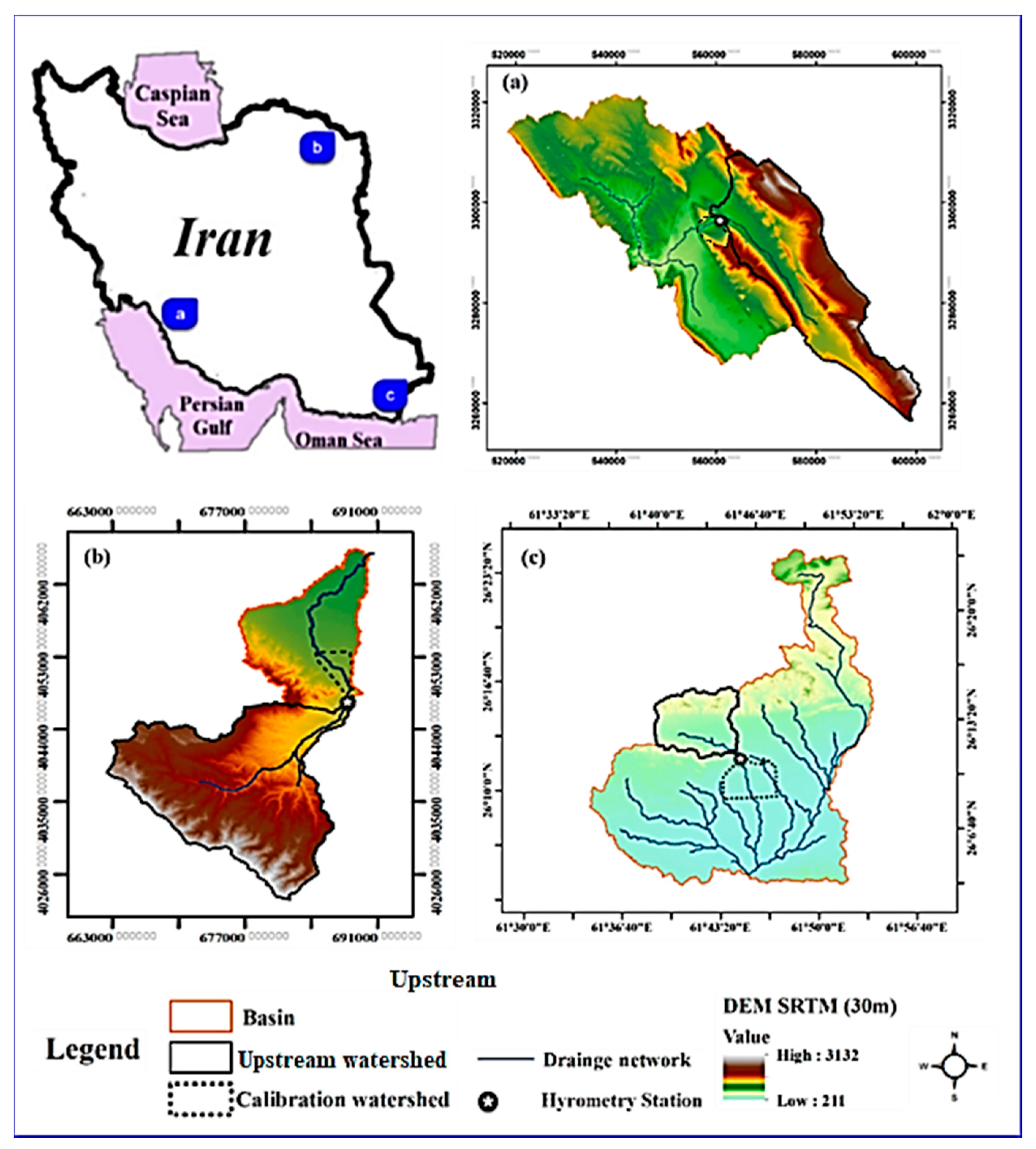
2.1. Study Area

This study focuses on the Frizi, Sarbaz, and Shapour basins in northeast, southeast, and south of Iran, respectively (Figure 1).

Table 1. The characteristics of Shapour basin and two alluvial fans of Frizi and Sarbaz.

	Annual Rainfall (mm)	Average Temperature (°C)	Relative Humidity (%)	Latitude	Longitude	Mean Elevation (m)	Watershed Area (km2)	Average Slope (%)
Sarbaz basin	90	35	21	29° 25′ N	38° 11′ E	267	628	1.03
	The upstream watershed of calibration area:					505	58.57	12
Frizi alluvial fan	372	15	42	20° 36′ N	58° 48′ E	1193	505	1.04
	The upstream watershed of calibration area:					2060	342.08	21
Shapour alluvial fan	510	23	49	29° 25′ N	51° 11′ E	1311	2031	13.88
	The upstream watershed of calibration area:					1695	718.6	16.8

provides the meteorological and physiographical characteristics of the study basins. Shapour basin is located in the Fars province with a semi-arid climate, Frizi basin is located on the northern slopes of the Binaloud Mountains in Khorasan Province with a semi-arid cold climate, and Sarbaz basin is located in the southern part of the Sistan and Baluchestan province with hot and dry climate. The areas delineated with dashed lines in Figure 1 represent designated areas for the calibration of models which in Shapour basin is a normal fluvial watershed with mountains and plains, and in Frizi and Sarbas basins are alluvial fan. Alluvial fans are triangular-shaped deposits of water-transported material where there is a rapid change in river slope and tend to be larger and more prominent in arid to semi-arid regions [23].

2.2. Input Data

2.2.1. Digital Elevation Model (DEM)

The Digital Elevation Model (DEM) is a digital map that contains the elevation of all points in a region. The DEM is usually produced and used as a raster structure in GIS software, where the value of each cell is the average height of a small piece of land. The DEM is widely used in physiographic studies and hydrology models, including the production of slope maps, the distribution of elevation changes, and sub-basin extraction [18]. DEM 30 m derived from Shuttle Radar Topography Mission (SRTM) is considered as one of the most accurate DEMs which are freely available [20]. Therefore, the DEMs of Frizi, Sarbaz, and Shapour basins were extracted from the USGS EarthExplorer website [24] and used in this study (Figure 1).

2.2.2. Hydrometric Data

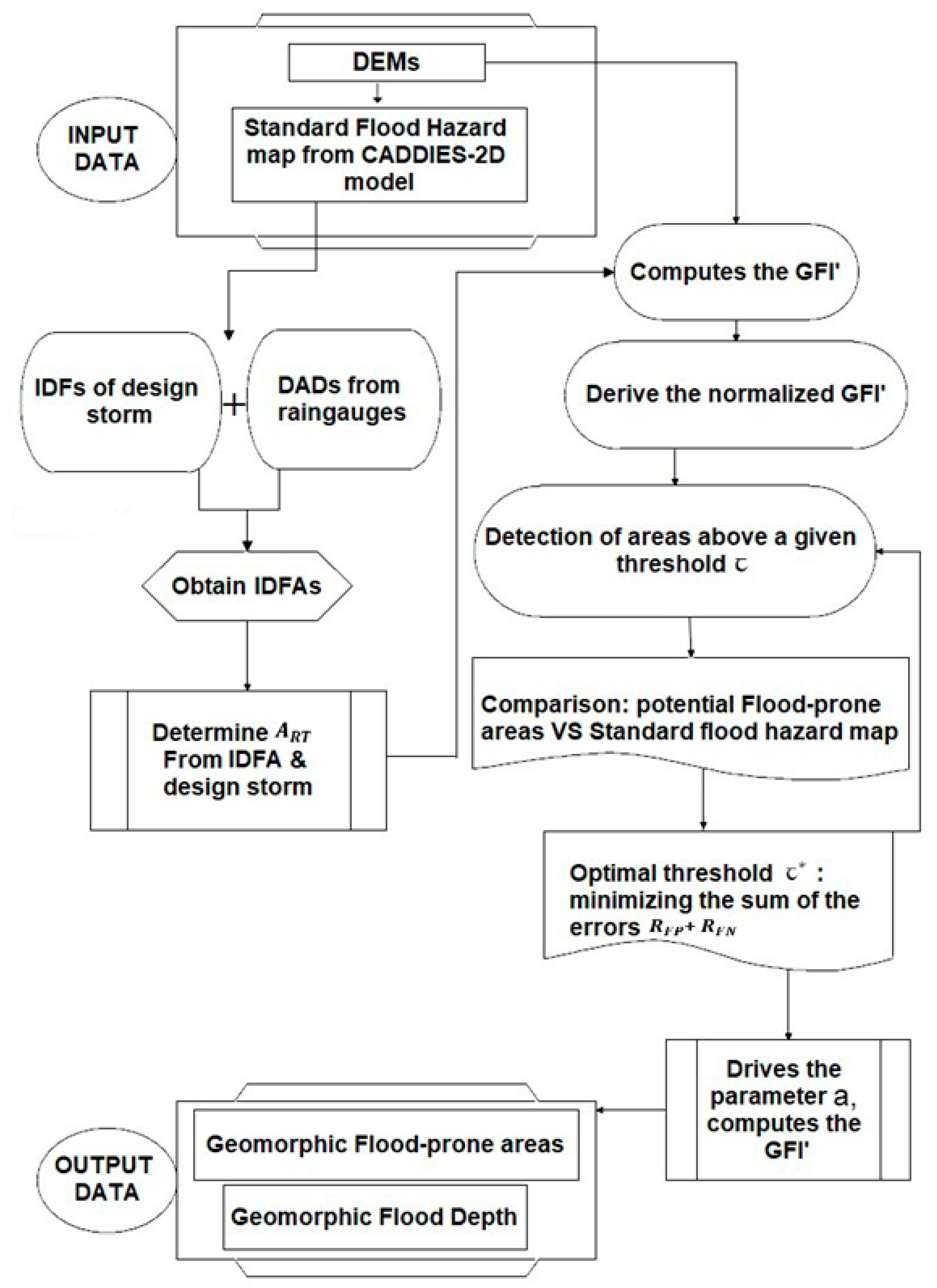
The discharge records from hydrometric stations are necessary for generating the design flood hydrographs, which in turn are necessary for delineating the standard flood maps. For the purpose of this study, a design flood with 100-year return period was selected. The maximum discharge of the design flood for the study basins was estimated using the data from hydrometric stations in the basins (Figure 1) and Gumbel probability distribution function. Finally, the design flood hydrographs of the study basins (Figure 2) were derived following the SCS runoff curve number method. The runoff curve number is an empirical parameter used in hydrology for predicting direct runoff or infiltration from rainfall excess developed by the USDA Natural Resources Conservation Service, a.k.a., the Soil Conservation Service or SCS [25]. This efficient method is widely used in determining the approximate amount of direct runoff from a rainfall event in a particular area [26,27].

Figure 2 depicts that for a 100-year return period flood, the Shapour basin has a hydrograph with a very high peak discharge whereas Frizi and Sarbaz fans have lower peak discharges due to the lower steepness in the alluvial fans. Figure 2 also shows that Sarbaz basin has the longest concentration time.

2.3. Methodology

In order to calibrate and validate the performance of GFI model in estimating flood plain extent and depth, first the CADDIES-2D hydraulic model generated the standard flood maps with a 100-year return period. Calibration of GFI model with CADDIES-2D provided a threshold to classify the whole basin into flooded and non-flooded areas. In addition, the novel concept of intensity-duration-frequency-area (IDFA) curves was introduced to confine the maximum hydrologically contributing area of a basin and improve the performance of GFI model. The flowchart of the presented methodology is illustrated in Figure 3 and different aspects of it are explained in more detail in the following sections.

The weighted cellular automata 2D (WCA2D) version of CADDIES-2D model was utilized to produce the standard flood maps. The WCA2D is a diffusive-like model that neglects inertia and momentum conservation terms which has the following major features [5]:

• The ratios of water conveyed from central to the downstream neighboring cells (intercellular-volume) are computed using a fast weight-based method;
• The water volume moved between the central cell and the neighbors is confined by the Manning’s and the critical flow equations;
• The adaptive time step and velocity, are both assessed within a larger updated time step to increase simulation speed and performance.

The WCA2D model is capable of working on grids with different neighborhood types and cells and it can perform parallel computations on a multi-core CPU and graphics card GPU which makes it very fast and suitable for near real time applications. The corresponding application of WCA2D model called CADDIES-caflood is publicly available on the webpage of the Centre for Water Systems at: http://cws.exeter.ac.uk.

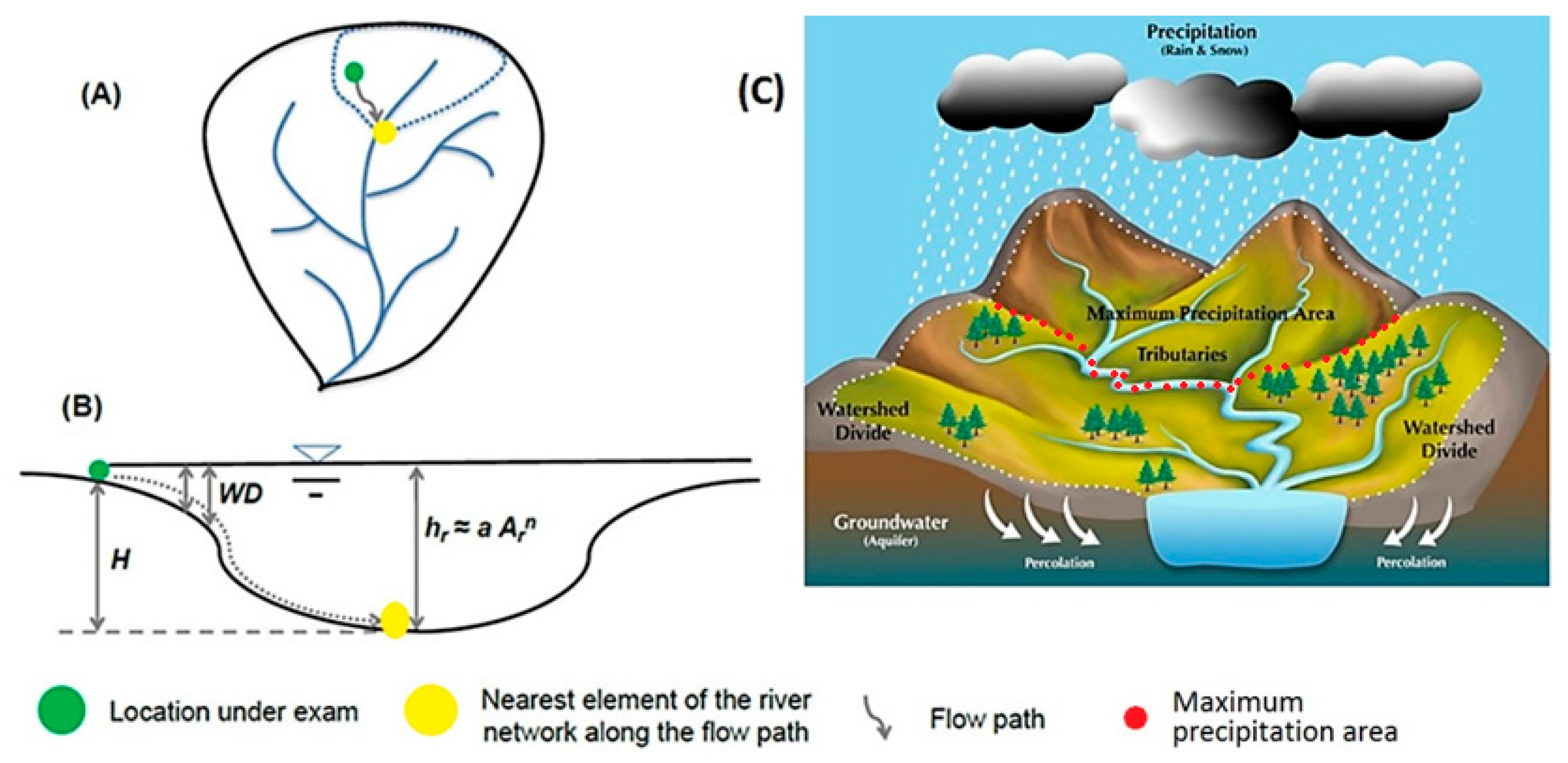
2.3.1. Geomorphic Flood Index (GFI)

According to Samela et al. [21], the amount of GFI at each study point (green dot in Figure 4a) is the natural logarithm of water depth (${\mathrm{h}}_{\mathrm{r}}$) in the hydrologically nearest waterway point (yellow dot in Figure 4a) to the elevation difference ($\mathrm{H}$) of those points (green and yellow dots in Figure 4b)

$$\mathrm{GFI}=\mathrm{Ln}\left(\frac{{\mathrm{h}}_{\mathrm{r}}}{\mathrm{H}}\right)$$

(1)

where ${\mathrm{h}}_{\mathrm{r}}$ is calculated as a function of the hydrologically participating area (dotted line in Figure 4a) upstream of the point under investigation ($A_r$) using a power relation developed by Nardi et al.:

$${\mathrm{h}}_{\mathrm{r}}={\mathrm{aA}}_{\mathrm{r}}^{\mathrm{n}}$$

(2)

where $\mathrm{a}$ and $\mathrm{n}$ are the parameters of power function and can be calibrated with the data of hydrometric stations in a region. According to Equation (1), the locations with GFI values ≥0 are located in the flood prone areas [28].

Manfreda et al. [28] demonstrated that parameter “$\mathrm{a}$” in Equation (2) does not affect the calibration results of flood prone areas and suggested that GFI can also estimate the maximum inundation depth by assuming a surrogate GFI (GFI’):

$${\mathrm{GFI}}^{’}=\mathrm{GFI}-\ln \left(\mathrm{a}\right)=\ln \left(\frac{A_r^n}{\mathrm{H}}\right)=\ln \left(\frac{{\mathrm{h}}_r}{aH}\right)$$

(3)

Given this definition, the linear binary classification is used to divide the range of GFI’ values in a basin into flooded and non-flooded classes using a threshold value (τ). The normalized GFI’ boundaries (i.e., −1 ≤ τ ≤ 1) should be used and iteratively revised the portion of the basin employed for calibration. For every threshold there is a potential flood-prone area binary map, which is collated to a standard floodplain map (Figure 5). The detailed information about the linear binary classification has been presented in the work of Samela et al. [1], but for computing the optimal normalized threshold, it should be minimizing the sum of the false positive rate and the false negative rate, imputing equal weights to the two amounts.

Therefore, the estimated optimal threshold, τ, can be used to derive the parameter a of the scaling function [28]:

$$a=\frac{1}{\exp \left(\mathsf{\tau }\right)}$$

(4)

Thereby, the values of river stage depth $h_r$ in Figure 4b can be estimated from Equation (2). Once the water level in the river network is estimated, the next task is to determine the water depth ($WD$) in the adjacent areas. For each point of the basin, the difference between the elevation ($H$) and the riverbed is determined (see Figure 4b). At this point, the $h_r$ values can be used to estimate the water depth ($WD$) on a cell by cell basis of the flood-prone areas, as in Equation (5) [28]:

$$WD=h_r-H$$

(5)

In order to implement the GFI, Samela et al. [22] provided Geomorphologic Flood Assessment (GFA) plug-in on QGIS software that can map the basin floodplain from a combination of geomorphological data extracted from the DEM layer, along with floodplain information usually available for part of the basin.

2.3.2. Modification of the Water Depth ($h_{\mathrm{r}}$)

According to Equation (2), the hydrologically contributing area ($A_r$) of a study point (blue dotted border in Figure 4a) can get accumulatively larger by moving downstream of a basin resulting in corresponding deeper river depths values ($h_r$). However, it should be considered that storms in a region with a certain return period have certain characteristics such as intensity and area of precipitation [29]. This fact is in contradiction with the assumption of GFI and parameter $A_r$, especially in large basins in arid and semi-arid regions. Therefore, it is suggested to put a limit on $A_r$ and change Equation (2) as below:

$$h_r\approx \{\begin{array}{cc}a{A}_r^n& if A_r<A_{RT}\\ a{A}_{RT}^n& if A_r\ge A_{RT}\end{array}$$

(6)

where, A_RT is the maximum precipitable area of a storm with a certain return period in the study area. In order to determine A_RT, it is suggested here to use the novel concept of intensity-duration-frequency-area (IDFA) curves of the storms in a study region.

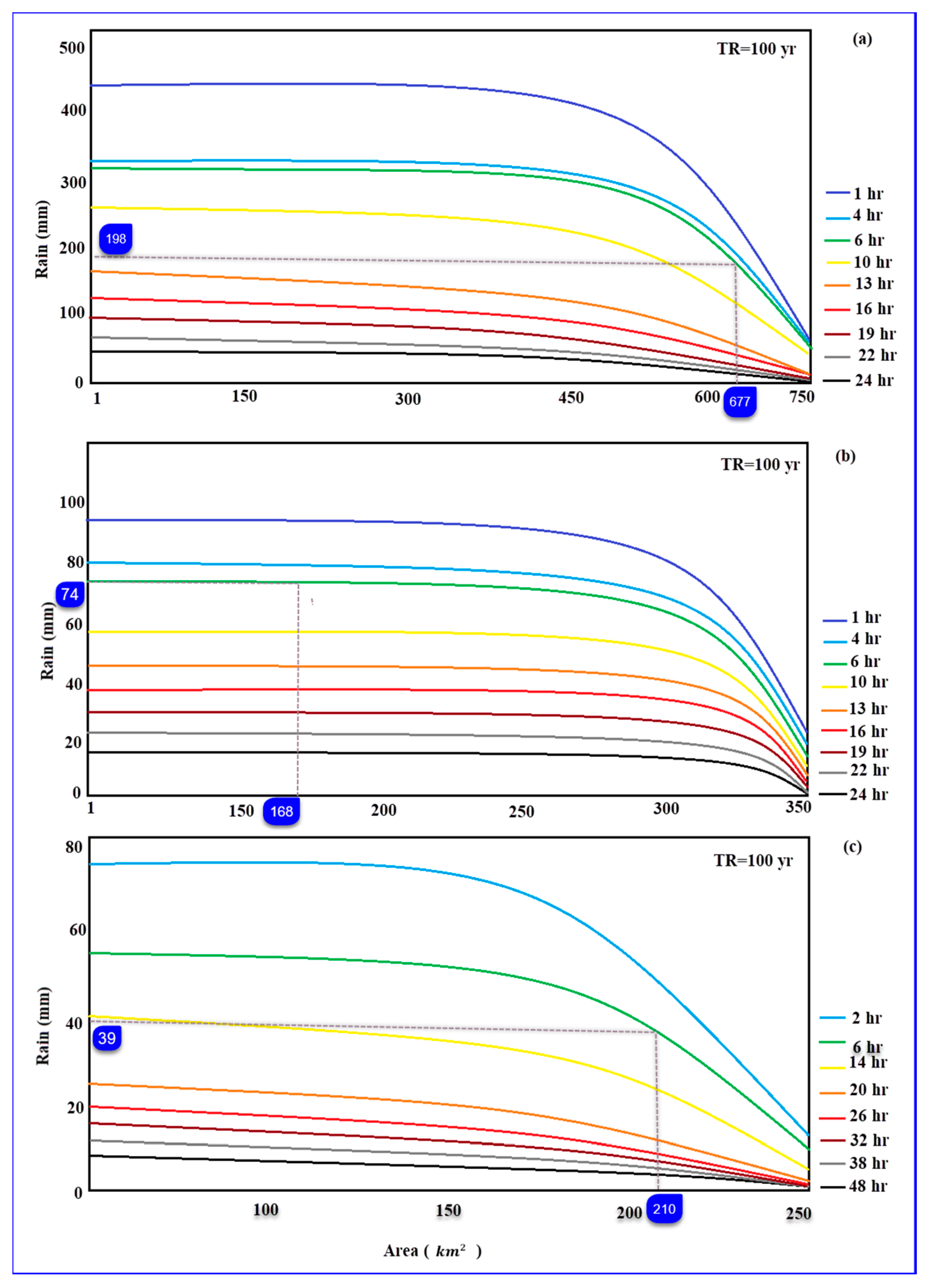
2.3.3. Intensity-Duration-Frequency-Area (IDFA) Curves

Historical records of rain gauges are necessary to determine rainfall characteristics of a basin. These characteristics are usually studied by developing intensity-duration-frequency (IDF) curves [30] and depth-area-duration (DAD) curves [31]. The IDFs are obtained by fitting a theoretical extreme value distribution (e.g., Gumbel Type I) to the rainfall records to estimate the rainfall events associated with given exceedance probabilities [32]. However, the development of DADs requires isohyet maps obtained from different methods such as: rainfall gradient, simple classic statistical methods, and/or complicated geostatistical methods. Hershfield and Wilson [33] suggested that the spatial pattern of a specific storm (i.e., DAD) follows:

$$\overline{P}=P_{max}{e}^{-k{A}^m}$$

(7)

where, $\overline{P}$ (mm) is the average rainfall depth over a specific area $A$ (km²); $P_{max}$ is the rainfall depth at the center of storm; and $k$ and $m$ are constant parameters that can be calibrated from the isohyet maps. While, IDFs provide temporal information about rainfall in a specific location, they do not give any information about rainfall spatial distribution, whereas DADs provide spatial information of a single storm. Therefore, it is suggested here to use a novel concept in hydrometeorology as intensity-duration-frequency-area (IDFA) curves introduced by Ghahreman [34] which represent all four necessary characteristics of precipitation in a basin. Rain gauge data within and around a basin can reveal rain centers; and regional IDFs (IDF_Regional) can be driven by interpolation techniques [35]. The average probable precipitation of the design storm with a certain return period ($\overline{P}$) can be calculated by multiplying corresponding duration and intensity values within the IDF_Regional curves. $P_{max}$ can then be infused into the DAD of the most intense storm recorded ever in that period. By calculating ($\overline{P}$/$P_{max}$) ratios for any desired area and applying it to all points on the IDF_Regional curves, the area dimension can be added to these curves. Thus, IDFAs can be used to determine the ART in Equation (6).

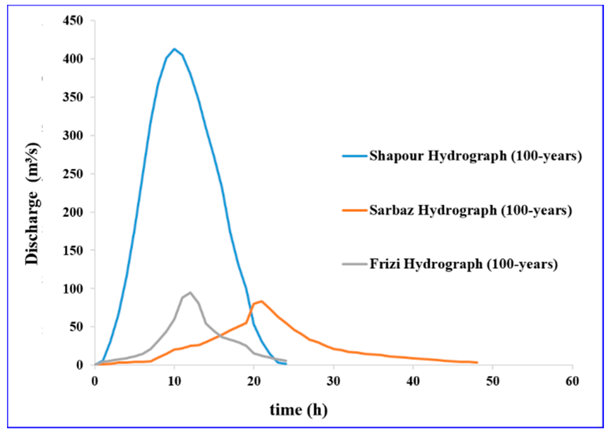
3. Results and Discussion

The methodology presented in this paper is implemented following the steps of Figure 3. In order to implement the GFA plug-in which is the corresponding application of GFI model, the required “DEM”, “Filled DEM”, “Flow direction”, and “Flow accumulation” maps of the study area, were obtained from DEM of SRTM (30 m) using the “Fill”, “Flow direction” and “Flow accumulation” tools of the Hydrology toolbox in the ArcMap software. In order to achieve to the standard flood maps for a small part of the study areas, CADDIES-caflood (which is the corresponding application of WCA2D model) was utilized. The inputs of the CADDIES-caflood were DEM map (Figure 1) and hydrograph (Figure 2) of the basin; and the outputs were flood depth (m) and velocity (m/s) of the study areas with spatial resolution of 30 m (Figure 6).

Figure 6 illustrates the 100-year flood-prone areas (a–c) and water depth results (d–f) of CADDIES-2D model for (1) Sarbaz, (2) Frizi, and (3) Shapour basins, respectively. According to Figure 6a,b, the avulsion phenomenon in the stream path has been modeled suitably by CADDIES-2D in the Sarbaz and Frizi alluvial fans. Avulsion is the sudden change in the river path during large floods which carry the necessary power to rapidly change the landscape and usually occurs in Alluvial fans [36]. Figure 6c shows a normal fluvial river with no apparent avulsion. Figure 6d–f illustrates the variation of water depth along the river in a 100-year flood. As can be seen, the water depth increased where the river encountered a pit, road, or in the meanders.

In the next step, the $A_{RT}$ constraint were imposed on $h_r$ (Equation (6)) to prevent the GFA model from producing accumulatively bigger river depth values. In order to calculate $A_{RT}$, the IDFAs of study areas were plotted in Figure 7 following Section 2.3.3 and information acquired from the most severe storm from rain gauges. Based on Figure 7, the $A_{RT}$ values for a 6-h design storm with the return period of 100 years were 677, 168, and 210 km² for Shapour, Frizi, and Sarbaz basins, respectively. Then, the standard flood maps (Figure 6a–c) were used to calibrate the GFI’ threshold (τ) in Equation (3) following the linear binary algorithm.

Having all the required inputs, the GFA outputs were the 100-year floodplain of study areas (Figure 8), and the performance metrics (

Table 2. The performance of linear binary classification of Geomorphologic Flood Assessment (GFA) model based on the Geomorphic Flood Index (GFI) and modified GFI.

Basin Name		τ a	RFP *	RTP **	RFP+(1 − RTP) ***	AUC b	Ratio of Calibration Area (%)
Sarbaz	Modified GFI	−0.25	0.11	0.17	0.94	0.42	2.45
	GFI	−0.24	0.12	0.16	0.95	0.40
Frizi	Modified GFI	−0.23	0.45	0.58	0.87	0.53	2.12
	GFI	−0.25	0.47	0.55	0.89	0.51
Shapour	Modified GFI	−0.28	0.10	0.98	0.12	0.96	2.83
	GFI	−0.30	0.11	0.95	0.14	0.93

^a optimal threshold value $\tau$, * false positive rate $R_{FP}$, ** true positive rate $R_{TP}$, *** sum of errors $R_{FP}+(1-R_{TP}$), and ^b area under the curve AUC for basin.

) including the calibrated threshold (τ), type 1 error (Rate of False Positive, $R_{FP}$), sensitivity (Rate of True Positive, $R_{TP}$), sum of errors ($R_{FP}$+ (1 − $R_{TP}$)), and model precision (area under the curve, AUC). Locations with GFI’ values bigger than τ are located inside the floodplain while smaller values are not considered as flood areas. The AUC equal to 1 represents 100% success in detecting flood prone areas with respect to the standard flood map [1]. According to Table 2, the constraint imposed on $h_r$ in the GFI model (Equation (6)) produced higher AUCs and lower R_FP + (1 − R_TP) values than the original model, which from here on is called the “modified GFI”. Moreover, it can be noted that the GFI model has a strong sensitivity in identifying flood-prone areas in the Shapour basin (with AUC = 0.93), and not outstanding sensitivity in the Sarbaz and Frizi basins (with AUC = 0.40 and 0.51, respectively). Samela et al. [21] suggest that the area envisaged for the calibration of the GFA model (i.e., the subbasin of the standard flood map) needs to be at least 2% of the whole study area, which for the Sarbaz, Frizi, and Shapour basins were 2.45, 2.12, and 2.83%, respectively.

Figure 8 illustrates the 100-year floodplains of the study areas as generated by CADDIES-2D, GFI and Modified GFI. In general, there was a good agreement between the maps generated by the standard hydraulic model and geomorphic method (Figure 8a,b,d,e,g,h) which has also been mentioned in the similar works [1,16,18,19,21]. However, the modified GFI seems to have more consistent results with the standard maps (Figure 8a,c,d,f,g,i) because of confining the maximum river depth. The comparison among the study areas (Figure 8a–i) also indicates that the GFA model generally performs better in fluvial rivers (Shapour basin, Figure 8g–i) than in alluvial fans (Sarbaz and Frizi, Figure 8a–f).

In order to achieve the potential GFI flood depth map of each study basin, the water level in each cell of the stream network was estimated from Equation (2) (the parameter a was calculated from Equation (4) and 𝜏 values in Table 2). Once the water level in the river network was estimated, the water depth (WD) in the adjacent areas were estimated from the difference in the elevation (H) between them and the river bed following Equation (5). Figure 9 compares the flood depth maps of the study areas as generated by the GFI and modified GFI models with the CADDIES-2D. In order to interpret Figure 9 properly, it should be noted that these models use two completely different structures to achieve the results and that the GFI flood depth maps are only complementary outputs and are not calibrated with the CADDIES-2D hydraulic depth simulations. The CADDIES-2D flood depth map is obtained from a specific simulation scenario and changing the scenario will produce different results depending on how factors such as hydrograph, time-step, and initial conditions have been determined; whereas the GFI model estimates the water depth at each different cell of a watershed individually and depending on the relative position of the studied cell to the river.

Figure 9 illustrates that, with some overestimation, the GFI model is able to capture the general trend of WD variations in comparison with the CADDIES-2D flood depth map. Similar studies have also mentioned that GFI overestimates the water depth [28,37], but comparing the second and third columns of Figure 9 shows that this problem is mitigated for the modified GFI as a result of imposing constraint on $h_r$ values. It is worth mentioning that the GFI performance in estimating the WD can be optimized to reach the minimum error if calibrated with a standard flood depth map (i.e., CADDIS-2D flood depth map). However, the purpose of this study was to achieve an estimate of the flood depth using only information about flood extend which is also available via remote sensing techniques. This means that the combination of the GFI method with satellite imagery can provide a unique opportunity for estimating both flood depth and extend in the near real-time and large scales.

Finally, the GFI calibrated thresholds (τ) were used in the rest of study areas to achieve complete 100-year floodplain maps (Figure 10). As can be seen in Figure 10, the flood prone areas even in the most remote regions of the study basins were delineated using only DEM maps which is useful for strategic decision making in less developed regions.

4. Conclusions

Conventional hydraulic methods of flood mapping require high computational capacities and multiple data sets, which make them not applicable in the large scales or ungauged regions despite their high accuracy. However, the results of these methods are available at smaller scales which can be generalized to large scales using geomorphological indices. Based on the literature, the GFI morphological flood index and its application GFA tool have the best performance in producing flood extents and also capable of giving a rough estimate of flood depth using only DEM maps and a standard flood map of a small portion of the study area.

The work in this paper implements the GFI model and enhances its performance through imposing the constraint of maximum precipitable area ($A_{RT}$) which is estimated through generating intensity-duration-frequency-area curves. The IDFAs are a novel concept in hydrometeorology which represent all four necessary characteristics of precipitation in a basin. The performance of developed method was demonstrated by application to the Frizi, Sarbaz, and Shapour basins in different parts of Iran. The inputs of this method are the DEM-SRTM-30 m and the 100-year standard floodplain derived from CADDIES-2D model, which is used to find the optimum threshold (τ) of the binary classification of the GFI values.

Based on the results, it can be concluded that the GFA model has a high ability to delineate flood extents in the fluvial and mountainous basins (Shapour basin), while it cannot model the avulsion phenomenon in the alluvial fans (Sarbaz and Frizi basins). In terms of flood depth, despite overestimation, the GFI model is able to capture the general trend in the water depth variations. Imposing constraint on the maximum precipitable area using the IDFAs allows for mitigating the overestimation of GFI and producing better flood depth results. Finally, the calibrated thresholds (τ) can be used to generalize the GFI results to the whole study area to achieve complete flood maps.

For the future works, it is suggested to calibrate the GFI model based on a standard flood depth map to minimize the errors in the spatial distribution of estimated flood depth. Using DEMs with resolutions less than 1 m (e.g., drone data) could help the GFI model to delineate stream branching in the alluvial fans as well. Moreover, the combination of satellite imagery with the GFI model can provide a unique opportunity for the flood risk assessment and crisis management in the near real-time and large scales, especially in the scarce-data regions. However, it should be noted that the geomorphic methods cannot be replaced with the common hydraulic models in some aspects, such as flood wave propagation.

References

1. Samela, C.; Troy, T.J.; Manfreda, S. Geomorphic classifiers for flood-prone areas delineation for data-scarce environments. Adv. Water Resour. 2017, 102, 13–28. [Google Scholar] [CrossRef]
2. Guidolin, M.; Duncan, A.; Ghimire, B.; Gibson, M.; Keedwell, E.; Chen, A.S.; Djordjevic, S.; Savic, D. CADDIES: A new framework for rapid development of parallel cellular automata algorithms for flood simulation. In Proceedings of the 10th International Conference on Hydroinformatics HIC, Hamburg, Germany, 14–18 July 2012. [Google Scholar]
3. Hunter, N.M.; Bates, P.D.; Horritt, M.S.; Wilson, M.D. Simple spatially-distributed models for predicting flood inundation: A review. Geomorphology 2007, 90, 208–225. [Google Scholar] [CrossRef]
4. Yen, B.; Tsai, C.-S. On noninertia wave versus diffusion wave in flood routing. J. Hydrol. 2001, 244, 97–104. [Google Scholar] [CrossRef]
5. Guidolin, M.; Chen, A.S.; Ghimire, B.; Keedwell, E.C.; Djordjević, S.; Savić, D.A. A weighted cellular automata 2D inundation model for rapid flood analysis. Environ. Model. Softw. 2016, 84, 378–394. [Google Scholar] [CrossRef] [Green Version]
6. Wolfram, S. Cellular automata as models of complexity. Nature 1984, 311, 419–424. [Google Scholar] [CrossRef]
7. Itami, R.M. Simulating spatial dynamics: Cellular automata theory. Landsc. Urban Plan. 1994, 30, 27–47. [Google Scholar] [CrossRef]
8. Dottori, F.; Todini, E. A 2D flood inundation model based on cellular automata approach. In Proceedings of the XVIII International Conference on Water Resources CMWR, Barcelona, Spain, 21–24 June 2010. [Google Scholar]
9. Dottori, F.; Todini, E. Developments of a flood inundation model based on the cellular automata approach: Testing different methods to improve model performance. Phys. Chem. Earthparts A/B/C 2011, 36, 266–280. [Google Scholar] [CrossRef]
10. Ghimire, B.; Chen, A.S.; Guidolin, M.; Keedwell, E.C.; Djordjević, S.; Savić, D.A. Formulation of a fast 2D urban pluvial flood model using a cellular automata approach. J. Hydroinform. 2013, 15, 676–686. [Google Scholar] [CrossRef] [Green Version]
11. Nardi, F.; Biscarini, C.; Di Francesco, S.; Manciola, P.; Ubertini, L. Comparing a large-scale DEM-based floodplain delineation algorithm with standard flood maps: The Tiber River Basin case study. Irrig. Drain. 2013, 62, 11–19. [Google Scholar] [CrossRef]
12. Chen, A.S.; Khoury, M.; Vamvakeridou-Lyroudia, L.; Stewart, D.; Wood, M.; Savic, D.A.; Djordjevic, S. 3D visualisation tool for improving the resilience to urban and coastal flooding in Torbay, UK. Procedia Eng. 2018, 212, 809–815. [Google Scholar] [CrossRef]
13. Wang, Y.; Liu, H.; Zhang, C.; Li, M.; Peng, Y. Urban Flood Simulation and Risk Analysis Based on Cellular Automaton. J. Water Resour. Res. 2018, 7, 360–369. [Google Scholar] [CrossRef]
14. Webber, J.L.; Burns, M.J.; Fu, G.; Butler, D.; Fletcher, T.D. Evaluating City Scale Surface Water Management Using a Rapid Assessment Framework in Melbourne, Australia. In New Trends in Urban Drainage Modelling, Proceedings of the International Conference on Urban Drainage Modelling, Palermo, Italy, 23–26 September 2018; Springer: Cham, Switzerland, 2018; pp. 920–925. [Google Scholar]
15. Arnaud-Fassetta, G.; Astrade, L.; Bardou, E.; Corbonnois, J.; Delahaye, D.; Fort, M.; Gautier, E.; Jacob, N.; Peiry, J.-L.; Piégay, H. Fluvial geomorphology and flood-risk management. Géomorphologie Relief Process. Environ. 2009, 15, 109–128. [Google Scholar] [CrossRef] [Green Version]
16. Manfreda, S.; Di Leo, M.; Sole, A. Detection of flood-prone areas using digital elevation models. J. Hydrol. Eng. 2011, 16, 781–790. [Google Scholar] [CrossRef]
17. Beven, K.J.; Kirkby, M.J. A physically based, variable contributing area model of basin hydrology/Un modèle à base physique de zone d’appel variable de l’hydrologie du bassin versant. Hydrol. Sci. J. 1979, 24, 43–69. [Google Scholar] [CrossRef] [Green Version]
18. Manfreda, S.; Samela, C.; Sole, A.; Fiorentino, M. Flood-prone areas assessment using linear binary classifiers based on morphological indices. In Vulnerability, Uncertainty, and Risk: Quantification, Mitigation, and Management; ASCE: Reston, VA, USA, 2014; pp. 2002–2011. [Google Scholar]
19. Manfreda, S.; Samela, C.; Gioia, A.; Consoli, G.G.; Iacobellis, V.; Giuzio, L.; Cantisani, A.; Sole, A. Flood-prone areas assessment using linear binary classifiers based on flood maps obtained from 1D and 2D hydraulic models. Nat. Hazards 2015, 79, 735–754. [Google Scholar] [CrossRef]
20. Samela, C.; Manfreda, S.; Paola, F.D.; Giugni, M.; Sole, A.; Fiorentino, M. DEM-based approaches for the delineation of flood-prone areas in an ungauged basin in Africa. J. Hydrol. Eng. 2016, 21, 06015010. [Google Scholar] [CrossRef]
21. Samela, C.; Manfreda, S.; Troy, T.J. Dataset of 100-year flood susceptibility maps for the continental US derived with a geomorphic method. Data Brief 2017, 12, 203–207. [Google Scholar] [CrossRef]
22. Samela, C.; Albano, R.; Sole, A.; Manfreda, S. A GIS tool for cost-effective delineation of flood-prone areas. Comput. Environ. Urban Syst. 2018, 70, 43–52. [Google Scholar] [CrossRef]
23. Cazanacli, D.; Paola, C.; Parker, G. Experimental steep, braided flow: Application to flooding risk on fans. J. Hydraul. Eng. 2002, 128, 322–330. [Google Scholar] [CrossRef]
24. JPL, N. NASA Shuttle Radar Topography Mission Global 1 arc second. Version 3. In NASA EOSDIS LP DAAC; USGS Earth Resources Observation and Science (EROS) Center: Sioux Falls, SD, USA, 2013. [Google Scholar]
25. Cronshey, R. Urban Hydrology for Small Watersheds; US Dept. of Agriculture, Soil Conservation Service, Engineering Division: Washington, DC, USA, 1986.
26. Woodward, D.E.; Hawkins, R.H.; Jiang, R.; Hjelmfelt, J.; Allen, T.; Van Mullem, J.A.; Quan, Q.D. Runoff curve number method: Examination of the initial abstraction ratio. In Proceedings of the World Water & Environmental Resources Congress, Philadelphia, PA, USA, 23–26 June 2003; pp. 1–10. [Google Scholar]
27. Zeng, Z.; Tang, G.; Hong, Y.; Zeng, C.; Yang, Y. Development of an NRCS curve number global dataset using the latest geospatial remote sensing data for worldwide hydrologic applications. Remote Sens. Lett. 2017, 8, 528–536. [Google Scholar] [CrossRef]
28. Manfreda, S.; Samela, C. A digital elevation model based method for a rapid estimation of flood inundation depth. J. Flood Risk Manag. 2019, 12, e12541. [Google Scholar] [CrossRef] [Green Version]
29. World Meteorological Organization. Manual for Depth-Area-Duration Analysis of Storm Precipitation; World Meteorological Organization: Geveva, Switzerland, 1969. [Google Scholar]
30. Pilgrim, D.; Cordery, I.; French, R. Temporal patterns of design rainfall for Sydney. Civ. Eng. Trans. 1969, CEII, 9–14. [Google Scholar]
31. Bureau, U.W. Manual for Depth-Area-Duration analysis of storm precipitation. Coop. Stud. Tech. Pap. 1946, 1, 99. [Google Scholar]
32. Koutsoyiannis, D.; Kozonis, D.; Manetas, A. A mathematical framework for studying rainfall intensity-duration-frequency relationships. J. Hydrol. 1998, 206, 118–135. [Google Scholar] [CrossRef]
33. Hershfield, D.M.; Wilson, W.T. A comparison of extreme rainfall depths from tropical and nontropical storms. J. Geophys. Res. 1960, 65, 959–982. [Google Scholar] [CrossRef]
34. Ghahreman, B. Derivation of Intensity-Duration-Frequency-Area (IDFA) Curves for Mashhad City. Comput. Methods Eng. 1998, 17, 69–81. [Google Scholar]
35. Myers, V.A.; Zehr, R.M. A Methodology for Point-to-Area Rainfall Frequency Ratios; Department of Commerce, National Oceanic and Atmospheric Administration: Silver Spring, MD, USA, 1980; Volume 55.
36. Mollaei, Z.; Davary, K.; Hasheminia, S.M.; Faridhosseini, A.; Pourmohamad, Y. Enhancing flood hazard estimation methods on alluvial fans using an integrated hydraulic, geological and geomorphological approach. Nat. Hazards Earth Syst. Sci. 2018, 18, 1159–1171. [Google Scholar] [CrossRef] [Green Version]
37. Albano, R.; Samela, C.; Crăciun, I.; Manfreda, S.; Adamowski, J.; Sole, A.; Sivertun, Å.; Ozunu, A. Large Scale Flood Risk Mapping in Data Scarce Environments: An Application for Romania. Water 2020, 12, 1834. [Google Scholar] [CrossRef]
Figure 1. The locations, digital elevation model (DEM) SRTM 30 m, hydrometry stations, and alluvial fans of the studied basins: (a) Shapour, (b) Frizi, and (c) Sarbaz, Iran.
Sustainability 12 07371 g001
Figure 2. The hydrographs of Frizi, Shapour and Sarbaz basins for a flood with 100-year return period.
Sustainability 12 07371 g002
Figure 3. The flowchart of proposed method to simultaneously generate flood extent and depth using geomorphologic indices.2.3.1. CADDIES-2D Hydraulic Model.
Sustainability 12 07371 g003
Figure 4. A schematic description of the parameters used to derive the Geomorphic Flood Index (GFI): (A) Dotted blue line shows the hydrologically contributing area ( A r ) of the study location (green circle); (B) the water depth (WD) estimated in a hypothetical cross-section (Manfreda et al., 2019); and (C) the concept of maximum precipitable area ( A R T ) delineated by the red dotted line which can be smaller than A r .
Sustainability 12 07371 g004
Figure 5. Linear binary classification.
Sustainability 12 07371 g005
Figure 6. The 100-year standard flood maps (ac) and flood depth maps (df) resulting from the CADDIES-2D model for the (1) Sarbaz fan; (2) Frizi fan; and (3) Shapour basin, Iran.
Sustainability 12 07371 g006
Figure 7. Intensity-duration-frequency-area (IDFA) curves for (a) Shapour, (b) Frizi, and (c) Sarbaz basins.
Sustainability 12 07371 g007
Figure 8. The floodplain limits from CADDIES-2D model (a,d,g), GFI (b,e,h), and modified GFI (c,f,i) for the (1) Sarbaz fan, (2) Frizi fan, and (3) Shapour basin.
Sustainability 12 07371 g008
Figure 9. Flow depth results of CADDIES-2D model (a,d,g), GFI (b,e,h), and modified GFI (c,f,i) for (1) Sarbaz fan; (2) Frizi fan; and (3) Shapour basin, Iran.
Sustainability 12 07371 g009
Figure 10. The modified GFI model output of flood prone areas for whole basin in (a) Sarbaz, (b) Frizi, and (c) Shapour.
Sustainability 12 07371 g010