Practical Performance Analysis of a Bifacial PV Module and System


Energy & Electrical Engineering, Korea Polytechnic University, Siheung-si 15073, Korea
*
Author to whom correspondence should be addressed.
Energies 2020, 13(17), 4389; https://doi.org/10.3390/en13174389
Submission received: 10 August 2020
/
Revised: 23 August 2020
/
Accepted: 24 August 2020
/
Published: 26 August 2020
(This article belongs to the Section A2: Solar Energy and Photovoltaic Systems)
Abstract
:Bifacial photovoltaic (PV) modules can take advantage of rear-surface irradiance, enabling them to produce more energy compared with monofacial PV modules. However, the performance of bifacial PV modules depends on the irradiance at the rear side, which is strongly affected by the installation setup and environmental conditions. In this study, we experiment with a bifacial PV module and a bifacial PV system by varying the size of the reflective material, vertical installation, temperature mismatch, and concentration of particulate matter (PM), using three testbeds. From our analyses, we found that the specific yield increased by 1.6% when the reflective material size doubled. When the PV module was installed vertically, the reduction of power due to the shadow effect occurred, and thus the maximum current was 14.3% lower than the short-circuit current. We also observed a maximum average surface temperature mismatch of 2.19 °C depending on the position of the modules when they were composed in a row. Finally, in clear sky conditions, when the concentration of PM 10 changed by 100 µg/m3, the bifacial gain increased by 4%. In overcast conditions, when the concentration of PM 10 changed by 100 µg/m3, the bifacial gain decreased by 0.9%.

1. Introduction
Nowadays, the market for bifacial photovoltaic (PV) modules and its applications is rapidly increasing. Moreover, the International Technology Roadmap for Photovoltaic (ITRPV) predicts that the global market share of bifacial PV cells will increase to 60% by 2029 [1].
A bifacial PV module can absorb irradiance on both sides. The performance of a bifacial PV module is influenced by module tilt and azimuth, similar to a monofacial PV module. It is, however, more influenced by the diffuse irradiance factor (DIF), height, and albedo than a monofacial PV module.
Bifacial PV modules have been analyzed in various installations and environmental conditions. Some studies have analyzed the output performance based on reflective materials such as white clothes, vegetables, and gravel [2,3]. There are also increasing applications of the bifacial PV module in a vertical form by integrating them into structures such as noise barriers and fences [4,5,6,7,8].
Previous studies have analyzed the simulated output performance, including the albedo, of bifacial modules based on the parameters of the installation setup, such as the tilt angle and height [9,10,11,12,13,14]. In addition, these simulated output performances were analyzed based on latitude and region, which affect environmental conditions [13,14]. Analyses of the output performance of bifacial PV modules at a vertical tilt were also carried out, but through simulations [15,16,17,18,19,20]. In general, before studies can take place, they are usually analyzed using simulations. The next step is to study bifacial PV modules in the field. Moreover, an energy performance analysis of a bifacial PV module in conditions with high particulate matter (PM) concentrations is yet to be published.
Therefore, in this study, we practically analyzed the performance of a bifacial PV module based on the installation setup and environmental conditions in the field. First, we analyzed the power performance of the bifacial PV module based on the size of the reflective material under the bifacial module. Second, we analyzed the power performance of the bifacial PV module when the module was installed vertically. Third, we analyzed the mismatch of the module surface temperatures when the modules were placed in a row. Finally, we analyzed the performance of the bifacial PV system in conditions with high PM concentrations. Each case was analyzed with a testbed. We collected the data using an on-site measurement and monitoring system.
2. Methods
2.1. Installation Conditions
Table 1 shows the experimental installation setup for each testbed.
Table 2 shows the specifications of the bifacial PV modules for the three testbeds. The bifacial PV module specifications at Testbed 1 are different from those at Testbeds 2 and 3.
Table 3 shows the specifications of the DC optimizer and the inverter at Testbed 3.
Table 4 shows the categories for the four experimental contents of the three testbeds. Testbeds 1 and 2 consist of a PV module and Testbed 3 consists of eight modules in a row.
Figure 1a shows the installation setup of Testbed 1. At Testbed 1, we evaluated the power performance of the bifacial PV module based on the size of the reflective material under the module.
Figure 1b shows the installation setup of Testbed 2. With this testbed, we analyzed the power performance of a vertical bifacial PV module based on the east (front)-west and west (front)-east orientations and the azimuth angle of the module.
Figure 1c shows the installation setup of Testbed 3. This testbed is composed of eight modules in a row and each module is connected with DC optimizers. We analyzed two conditions with this testbed. One analysis involved the temperature mismatch of the bifacial PV modules based on their positions. The other analysis involved the effects of particulate matter concentration levels of PM 2.5 and PM 10 on the diffuse irradiance factor and bifacial gain.
2.2. Measurement Equipment
Table 5 shows the specifications of the irradiance sensors, outdoor test measurement equipment, and PM data source. We analyzed performance of bifacial PV system through measurement experiments. As presented Table 5, we used different measurement experiment depending on experimental contents (Section 3.1: size of ground reflective material, Section 3.2: vertical installation of PV module, Section 3.3: mismatch in module temperature, Section 3.4: effect of particle pollution). The concentration of PM is collected nearby (1 km) the testbed.
3. Experimental Results
3.1. Size of Ground Reflective Material
The albedo is the most influenced parameter by rear-side irradiance. The ground albedo under the PV module is influenced not only by the type, but also by the size and age of the material as well as the presence of dirt on the reflective material underneath the module [21,22].
The irradiance incident on a module’s rear surface in a shaded area is less influenced by the reflective material than that for a rear surface in a non-shaded area. Figure 2 shows the size of the material for the two cases evaluated in this experiment. Testbed 1 is installed with a 37° tilt angle and a 0° (south) azimuth angle. Figure 2 also shows the plan view of each case at Testbed 1 where the blue square represents the module and the gray square with gray diagonal lines represents the reflective material.
In Case 1, the size of the reflective material was set to match the boundary of the non-shaded area at noon during the winter solstice when the shadow produced by the module was at its largest. In Case 2, the size of the material was chosen to be twice as large as Case 1 to contain the shaded area. The albedo of the reflective material in each case was 55%.
Figure 3 shows the specific yield comparison for both Cases 1 and 2 based on the size of the reflective material. As depicted by the graph, we measured the output power of the bifacial PV module from 10:00 a.m. to 16:00 p.m. every 30 min. We also observed a deviation of the output power for the bifacial PV module. The performance of the bifacial module was higher in Case 2 than that in Case 1, even though Case 2 included the shaded area. The average deviation of the specific yield was 1.6%.
From these experiments, we confirmed that an increase in the size of the reflective material area increased the performance of the bifacial PV module. The rear-surface irradiance of the bifacial module was influenced not only by being at the underside of the PV module, but also by the surrounding area. This testbed was composed of only one module. Therefore, we found that the irradiance at the rear side was more affected by the surrounding area.
3.2. Vertical Installation of PV Module
The installation azimuth of the bifacial PV module was considered not only for the south-facing orientation, but also east-west orientation for the vertical installation setup.
We analyzed the output performance based on the bifaciality factor of the bifacial PV module. As indicated by the bifaciality factor, the efficiency of the bifacial PV modules on each side was different. However, the azimuth to be used for the front side must still needed be determined. Therefore, we divided the case into two conditions, as follows:
- east (front)-west
- west (front)-east
The albedo was 23% for each case and the bifaciality factor of the bifacial PV module was 82%.
Figure 4 shows the specific yield based on the bifacial PV module’s azimuth angle relative to the front panel. The efficiency of the bifacial PV module was different for each surface, and the graph indicates this difference for each installation setup. The output performance of the module with the east (front)-west orientation demonstrated a high specific yield in the morning, whereas the output performance of the module with the west (front)-east orientation demonstrated a high specific yield in the afternoon.
Figure 5 shows the I–V curve for each orientation of the vertically installed bifacial PV module. The curves for the two conditions indicate a step I–V curve before and after 13:30 p.m. More specifically, the I–V curve for the module with the east (front)-west orientation shows a step curve at 14:30 p.m., whereas the I–V curve for the module with the west (front)-east orientation shows a step curve at 12:30 p.m.
A shadow was produced by the module structure, which led to power losses [23]. Figure 6 shows the rear surface shading of the bifacial PV module corresponding to the I–V curves in Figure 5. Here, we can observe the shadows produced on the rear side of the module. The I–V curve in Figure 5a indicates a step curve due to a shadow created by the junction box and the module frame, as depicted in Figure 6a. Similarly, the I–V curve in Figure 5b shows a step curve due to the shadow produced by the module frame, as depicted in Figure 6b. From Figure 5 and Figure 6, it is evident that shadows are produced on the rear surface of the bifacial PV module by the junction box and the module frame. This is because the junction box and module frame are not fully hidden in the rear surface of the module, resulting in the shadows observed on the rear surface due to the positioning of the module and the angle of the sun.
Table 6 shows the measured I–V curve data at 14:30 p.m. and 12:30 p.m. When we measured a PV module I–V curve in normal conditions, the maximum current was similar to the short-circuit current. Therefore, we compared the maximum current with the short-circuit current of the bifacial PV module at each orientation.
As presented in Table 6, the maximum current was 14.0% lower than the short-circuit current for the module with the east (front)-west orientation at 14:30 p.m. However, the maximum current for the module with the west (front)-east orientation was 5.3% lower than the short-circuit current.
The maximum current was 4.8% lower than the short-circuit current for the module with the east (front)-west orientation at 12:30 p.m., whereas the maximum current for the module with the west (front)-east orientation was 14.5% lower than the short-circuit current.
To summarize, when a shadow was produced on the rear surface of the bifacial PV module, the maximum current was on average 14.3% lower than the short-circuit current. However, when a shadow was not produced on the rear surface of the bifacial PV module, the maximum current was on average 5.1% lower than the short-circuit current.
3.3. Mismatch in Module Temperature
Irradiance mismatch in a module can occur depending on the module installation, as well as its positioning within a row. The surface temperature of a module changes with irradiance [24]. Therefore, we measured the surface temperature of the modules in the row to determine the module temperature mismatch.
Figure 7 shows the modules for which the temperature was measured. Because the mismatch of module temperature can differ depending on the location, we divided the measurements into the following two conditions.
We selected the module that was less affected by the module structure and considered the performance deviation according to the location in the row. Each experiment was performed based on the time when the sun’s azimuth angle coincided with the module installation’s azimuth angle (south-west 37°; summer 11:00 a.m.–15:00 p.m. and winter: 13:00 p.m.–17:00 p.m.).
Figure 8 shows the module surface temperatures for the summer and winter seasons. is the azimuth of the sun’s position and is the azimuth of the module’s position. The average deviation of the module surface temperature for Case 1 (neighboring modules) was 0.4 °C in the summer and 0.53 °C in the winter. The average deviation of the module surface temperatures for Case 2 (Distant modules) was 0.86 °C in the summer and 2.19 °C in the winter. Both cases reported a higher temperature deviation in the winter.
As shown in Figure 8, the module temperature deviation of Case 1 was smaller than that of Case 2 for both the summer and winter seasons. This was a result of the modules being situated in a row of one line.
Figure 9 shows the shadow locus for each season. Before the sun’s azimuth angle coincided with the module installation’s azimuth angle, there was a shadow under module No. 8. After the alignment of the azimuth angles, the shadow was cast under module No. 2. The size of the shadow was different for each season and hour. This shadow reduced the irradiance on the rear surface of the module and a reduced irradiance resulted in a lower temperature for that module. Therefore, the module temperature mismatch was different depending on the location of the module. Furthermore, the deviation of the module temperatures was higher in the winter.
Figure 10 shows the daily specific yield comparison between the modules on two specific days, one in the summer and one in the winter. Module No. 8 achieved the highest energy yield among the three evaluated modules. The deviation of the daily energy yield for Case 1 (Neighboring modules) was 0.06 kW/kWp in the summer and 0.1 kW/kWp in the winter. The deviation of the daily energy yield for Case 2 (Distant modules) was 0.08 kW/kWp in the summer and 0.28 kW/kWp in the winter. A higher specific yield deviation was reported for both cases in the winter.
3.4. Effects of Particle Pollution
Nowadays, the concentration of particle pollution, also called particulate matter (PM), has been increasing in the Republic of Korea. PM is generally identified into two categories, PM 2.5 and PM 10, depending on the size of the particles. PM 2.5 and PM 10 are the particle pollution where the size of particles is smaller than 2.5 μm and 10 μm, respectively. PM reduces the direct irradiance and thus the global horizontal irradiance (GHI) received by a module surface [24].
We analyzed the performance based on the diffuse irradiance factor. The diffuse irradiance factor (DIF) is the ratio of diffuse horizontal irradiance and GHI [25], and is affected by the amount of clouds and the position of the sun. To reduce the effects of other factors, we added the following criteria:
- Elevation of sun > 10°
- Exclude rainy days
A clearness index (kt) was also applied and is divided into three categories, namely: clear, partly cloudy, and overcast [26].
In this study, we distinguished between two cases according to the kt value in order to analyze the performance of the bifacial PV system based on the PM concentration under different sky conditions.
- Clear sky
- Overcast
We analyzed the output performance of the module using monitoring data from 1 January 2019 to 28 February 2019, a period in which the PM concentration was high. The kt is calculated as inversely proportional to GHI and extraterrestrial irradiance (I0), and it is affected by the solar altitude angle (β). The kt is defined as following formula [26].
Figure 11 shows the DIF based on the concentration of PM. As the concentration of PM increases, the DIF tends to increase. This is because the particles halt direct irradiance, but they distribute the irradiance in the air. The concentration of PM was obtained from a website supported by the Ministry of Environmental Sciences. Additionally, data regarding the GHI, DHI, and power of the bifacial PV module were measured using a data logger located in our university.
Table 7 shows DIF based on the concentration of PM at specific points. In clear sky conditions, when the concentration of PM 2.5 changed from 0 µg/m3 to 150 µg/m3, we observed that the DIF changed from 19.77% to 57.27%. Similarly, when the concentration of PM 10 changed from 0 µg/m3 to 100 µg/m3, we observed a change in DIF from 18.27% to 34.27%. The reason for this is that the PM 2.5 and PM 10 particles distributed the irradiance. As the concentration of PM 10 and PM 2.5 increased, the pollution particles produced more distribute irradiance [25].
In overcast conditions, when the concentration of PM 2.5 changed from 0 µg/m3 to 150 µg/m3, we observed that the DIF changed from 95.7% to 101.7%. In contrast, when the concentration of PM 10 changed from 0 µg/m3 to 100 µg/m3, we observed a change in the DIF from 98.68% to 96.68%. These results indicate that DIF increased when the concentration of PM increased.
When the sky conditions were clear, the difference in the DIF due to the increase in concentration levels of PM 2.5 and PM 10 was 37.28% and 16%, respectively. Otherwise, when the sky conditions were overcast, the deviation of the DIF due to the increase in PM concentration levels was less than 6%. Furthermore, the DIF in the overcast conditions was observed to be over 90%, regardless of the concentration level and size of PM. These results indicate that when the PM concentration levels increased, clear sky conditions had a larger effect on the change in the DIF than overcast conditions, in which the change in the DIF was much less. The size of the particles for PM 2.5 and PM 10 was smaller than the size of the water vapor molecules in the clouds. Therefore, the effect of the water vapors on the DIF was observed to be larger than that of the PM.
Figure 12 and Table 8 show the bifacial gain based on the concentration of PM. As the concentration of PM increased, the bifacial gain tended to increase. This is because the performance of the bifacial gain depends on the concentration of PM. A higher DIF resulted in a higher value for the irradiance, which reached the rear surface of the module, even though the direct irradiance was reduced.
In clear sky conditions, when the concentration of PM 2.5 changed from 0 µg/m3 to 150 µg/m3, we observed that the bifacial gain changed from 32.01% to 38.1%. When the concentration of PM 10 changed from 0 µg/m3 to 100 µg/m3, we observed that the bifacial gain changed from 31.03% to 35.03%.
In overcast conditions, when the concentration of PM 2.5 changed from 0 µg/m3 to 150 µg/m3, we observed that the bifacial gain changed from 50.16% to 50.91%. When the concentration of PM 10 changed from 0 µg/m3 to 100 µg/m3, we observed that the bifacial gain changed from 51.2% to 50.3%.
The deviation of the bifacial gain due to the increase in PM concentration levels for PM 2.5 and PM 10 was 6.09% and 4%, respectively, in clear sky conditions. In overcast conditions, the deviation of the bifacial gain due to the increase in PM concentration levels for PM 2.5 and PM 10 was 0.75% and −0.9%, respectively. A high DIF was observed in overcast conditions, regardless of the size of the particulate matter, whether PM 2.5 or PM 10. Therefore, a bifacial gain was also present regardless of the PM size.
4. Conclusions
In this study, we experimented with a bifacial PV module and a bifacial PV system by varying the size of the reflective material, vertical installation, positions of the modules for temperature mismatch, and concentration of PM using three testbeds.
First, we found that the wider the area of the reflective material, the better the output performance of the bifacial PV module at Testbed 1. When the size of the material was doubled to contain the shaded area, as in Case 2 relative to Case 1, the power performance of the bifacial PV module was observed to be 1.6% higher.
Second, we evaluated the power performance of the bifacial PV module in a vertical installation setup. The bifacial PV module power performance was higher for the module with the east (front)-west orientation than that with the west (front)-east orientation in the morning. In addition, the bifacial PV module power performance was higher for the module with the west (front)-east orientation than that with the east (front)-west orientation in the evening. Therefore, it is necessary to choose the appropriate azimuth angle for the bifacial module’s front surface based on the location the bifacial modules are installed at. Furthermore, we observed a shadow at the module’s rear surface produced by the junction box and the module frame, which resulted in a step I–V curve for the module as opposed to a normal I–V curve. When this shadow was produced on the rear side of the bifacial PV module, the maximum current of the I–V curve was on average 14.3% lower than the short-circuit current.
Third, a module temperature mismatch between neighboring modules and distant modules was observed in both the summer and winter seasons. When the modules were positioned nearby within a row, the deviation of the bifacial PV module surface temperature was observed to be 0.4 °C in summer and 0.53 °C in winter. However, when the bifacial PV modules were positioned distantly within a row, the deviation of the module surface temperature was observed to be 0.86 °C in the summer and 2.19 °C in the winter. This is caused by the shadow on the ground at each hour, according to the shadow locus analysis. Also, the deviation of the daily specific yield was observed to be 0.06 kW/kWp in the summer and 0.1 kW/kWp in the winter for the case of the neighboring modules. However, when the evaluated bifacial PV modules were positioned distantly within a row, the deviation of the daily energy yield was observed to be 0.08 kW/kWp in summer and 0.28 kW/kWp in winter. Similar to the deviation of the module surface temperatures, the deviation of the energy yield was observed to be higher in winter.
Finally, we observed that both the DIF and the bifacial gain increased when the concentration levels of PM increased in clear sky conditions. When the concentration of PM 2.5 reached 150 µg/m3, the DIF value increased from 19.77% to 57.27%, and the bifacial gain increased from 32.01% to 38.10%. When the concentration of PM 10 increased to 100 µg/m3, the DIF value increased from 18.27% to 34.27% and the bifacial gain increased from 31.03% to 35.03%. In the overcast conditions, when the concentration of PM 2.5 reached 150 µg/m3, the DIF value increased from 95.7% to 101.7% and the bifacial gain increased from 50.16% to 50.91%. When the concentration of PM 10 was increased to 100 µg/m3, the DIF value decreased from 98.68% to 96.68% and the bifacial gain decreased from 51.2% to 50.3%. In recent years, the installation of bifacial PV systems has increased.
This paper can be used as an example to optimize the energy performance of bifacial PV systems based on the installation setup and environmental conditions.
Author Contributions
Conceptualization, J.J. and K.L.; formal analysis, J.J.; investigation, J.J.; resources, K.L.; data curation, J.J.; writing (original draft preparation), J.J.; writing (review and editing), J.J. and K.L.; visualization, J.J.; supervision, K.L.; project administration, K.L.; funding acquisition, K.L. All authors have read and agreed to the published version of the manuscript.
Funding
This researched was funded by the “Energy R&D Program” of the Korea Institute of Energy Technology Evaluation and Planning, grant no. 20173030068990, and by the Korea Electric Power Corporation, grant no. R17XA05-40.
Conflicts of Interest
The authors declare no conflict of interest.
References
- ITRPV. International Technology Roadmap for PV(ITRPV) 2018 Results, Version 10. Available online: https://itrpv.vdma.org/en/ (accessed on 1 October 2019).
- Kenny, P.; Lopez-Garcia, J.; Menendez, E.G.; Haile, B.; Shaw, D. Characterizing Bifacial Modules in Variable Operating Conditions. In Proceedings of the WCPEC, Waikoloa Village, HI, USA, 10–15 June 2018; pp. 1210–1214. [Google Scholar]
- Baumann, T.; Nussbaumer, H.; Klenk, M.; Dreisiebner, A.; Carigiet, F.; Baumgartner, F. Photovoltaic systems with vertically mounted bifacial PV modules in combination with green roofs. Sol. Energy 2019, 190, 139–146. [Google Scholar] [CrossRef]
- Mahmud, M.S.; Rahman, M.W.; Lipu, M.S.H.; Mamun, A.A. Solar Highway in Bangladesh Using Bifacial PV. In Proceedings of the ICSCA, Pondicherry, India, 6–7 July 2018; pp. 1–7. [Google Scholar]
- Faturrochman, G.J.; de Jong, M.M.; Santbergen, R.; Folkerts, W.; Zeman, M.; Smets, A.H.M. Maximizing annual yield of bifacial photovoltaic noise barriers. Sol. Energy 2018, 162, 300–305. [Google Scholar] [CrossRef]
- Khan, M.R.; Hanna, A.; Sun, X.; Alam, M.A. Vertical bifacial solar farms Physics, design, and global optimization. Appl. Energy 2017, 206, 240–248. [Google Scholar] [CrossRef] [Green Version]
- Meyer, C. Agro PV-Next2Sun’s vertical installations. In Proceedings of the Bifi PV Workshop, Amsterdam, The Netherlands, 16 September 2019. [Google Scholar]
- de Jong, M.M.; Kester, J.; van der Graaf, D.; Verkuilen, S.; Folkerts, W. Building the world’s largest bifacial solar noise barrier. In Proceedings of the EUPVSEC, Brussels, Belgium, 7–11 September 2018; pp. 1493–1495. [Google Scholar]
- Mermoud, A.; Wittmer, B. Yield simulations for horizontal axis trackers with bifacial PV modules in PVsyst. In Proceedings of the EUPVSEC, Brussels, Belgium, 7–11 September 2018; pp. 1929–1934. [Google Scholar]
- Yusufoglu, U.A.; Lee, T.H.; Pletzer, T.M.; Halm, A.; Koduvelikulathu, L.J.; Comparotto, C.; Kopecek, R.; Kurz, H. Simulation of energy production by bifacial modules with revision of ground reflection. Energy Procedia 2014, 55, 389–395. [Google Scholar] [CrossRef] [Green Version]
- Chudinzow, D.; Haas, J.; Diaz-Ferran, G.; Moreno-Leiva, S.; Eltrop, L. Simulating the energy yield of a bifacial photovoltaic power plant. Sol. Energy 2019, 183, 812–822. [Google Scholar] [CrossRef]
- Kreinin, L.; Bordin, N.; Karsenty, A.; Drori, A.; Grobgeld, D.; Eisenberg, N. PV module power gain due to bifacial design. Preliminary experimental and simulation data. In Proceedings of the IEEE PVSC, Honolulu, HI, USA, 20–25 June 2010; pp. 2171–2175. [Google Scholar]
- Kreinin, L.; Karsenty, A.; Grobgeld, D.; Eisenberg, N. PV systems based on bifacial modules: Performance simulation vs. design factors. In Proceedings of the IEEE PVSC, Portland, OR, USA, 5–10 June 2016; pp. 2688–2691. [Google Scholar]
- Sun, X.; Khan, M.R.; Deline, C.; Alam, M.A. Optimization and performance of Bifacial Solar Modules A global perspective. Appl. Energy 2018, 212, 1601–1610. [Google Scholar] [CrossRef] [Green Version]
- Patel, M.T.; Khan, M.R.; Sun, X.; Alam, M.A. A worldwide cost-based design and optimization of tilted bifacial solar farms. Appl. Energy 2019, 247, 467–479. [Google Scholar] [CrossRef] [Green Version]
- Guo, S.; Walsh, T.M.; Peters, M. Vertically mounted bifacial photovoltaic modules A global analysis. Energy 2013, 61, 447–454. [Google Scholar] [CrossRef]
- Appelbaum, J. Bifacial photovoltaic panels field. Renew. Energy 2016, 85, 338–343. [Google Scholar] [CrossRef]
- Pbara, S.; Konnon, D.; Utsugi, Y.; Morel, J. Analysis of output power and capacity reduction in electrical storage facilities by peak shift control of PV system with bifacial modules. Appl. Energy 2014, 128, 35–48. [Google Scholar]
- Asgharzadech, A.; Marion, B.; Deline, C.; Hansen, C.; Stein, J.S. A sensitivity study of the impact of installation parameters and system configuration on the performance of bifacial PV arrays. IEEE J. Photovolt. 2018, 8, 798–805. [Google Scholar] [CrossRef]
- Asgharzadech, A.; Deline, C.; Stein, J.; Toor, F. A comparison study of the performance of South/North-facing vs East/West-facing Bifacial Modules under shading conditions. In Proceedings of the WCPEC, Waikoloa Village, HI, USA, 10–15 June 2018; pp. 1730–1734. [Google Scholar]
- Jaubert, J.N. Layout optimization of albedo enhancer materials used in bifacial PV systems. Presented at the Bifi PV Workshop, Amsterdam, The Netherlands, 16 September 2019. [Google Scholar]
- Yusufoglu, U.A.; Pletzer, T.M.; Koduvelikulathu, L.J.; Comparotto, C.; Kopecek, R.; Kurz, H. Analysis of the Annual Performance of Bifacial Modules and Optimization Methods. IEEE J. Photovolt. 2015, 5, 320–328. [Google Scholar] [CrossRef]
- Mühleisen, W.; Neumaier, L.; Hirschl, C.; Löschnig, J.; Bende, E.; Zamini, S.; Újvári, G.; Mittal, A. Optimization and design issues of bifacial PV modules and systems. In Proceedings of the EUPVSEC, Marseille, France, 9 September 2019; pp. 991–994. [Google Scholar]
- Hansen, C.; Riley, D.; Deline, C.; Toor, F.; Stein, J. A Detailed Performance Model for Bifacial PV Modules. In Proceedings of the EUPVSEC, Sandia National Lab (SNL-NM), Albuquerque, NM, USA, 26 September 2017; Available online: https://www.osti.gov/ (accessed on 4 December 2018).
- Kosmopoulos, P.G.; Kazadzis, S.; Taylor, M.; Athanasopoulou, E.; Speyer, O.; Raptis, P.I.; Amiridis, V. Dust impact on surface solar irradiance assessed with model simulations, satellite observations and ground-based measurements. Atmos. Meas. Tech. 2017, 10, 2435–2453. [Google Scholar] [CrossRef] [Green Version]
- Lee, H.Y.; Yoon, S.H.; Park, C.S. The Effect of Direct and Diffuse Split Models on Building Energy Simulation. J. Arch. Inst. Korea Plan. Des. 2015, 31, 221–229. [Google Scholar]
Figure 1.
Installation set of testbeds: (a) installation set of Testbed 1; (b) installation set of Testbed 2; (c) installation set of Testbed 3.
Figure 1.
Installation set of testbeds: (a) installation set of Testbed 1; (b) installation set of Testbed 2; (c) installation set of Testbed 3.
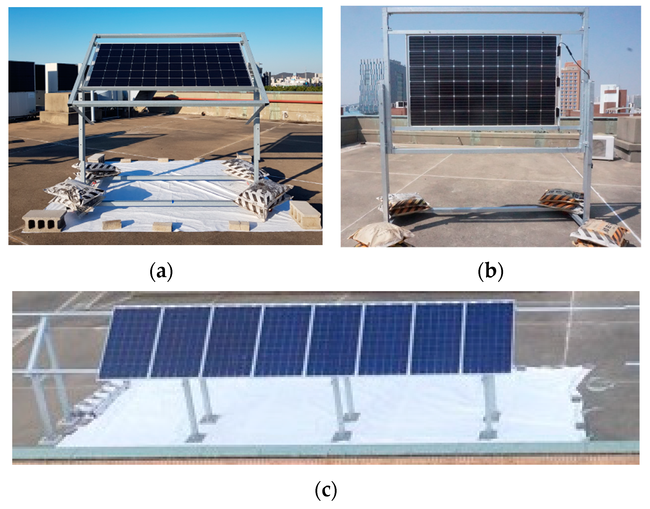
Figure 2.
Plan view of each case at Testbed 1.

Figure 3.
Specific yield for each case and power deviation.

Figure 4.
Specific yield based on front side orientation.
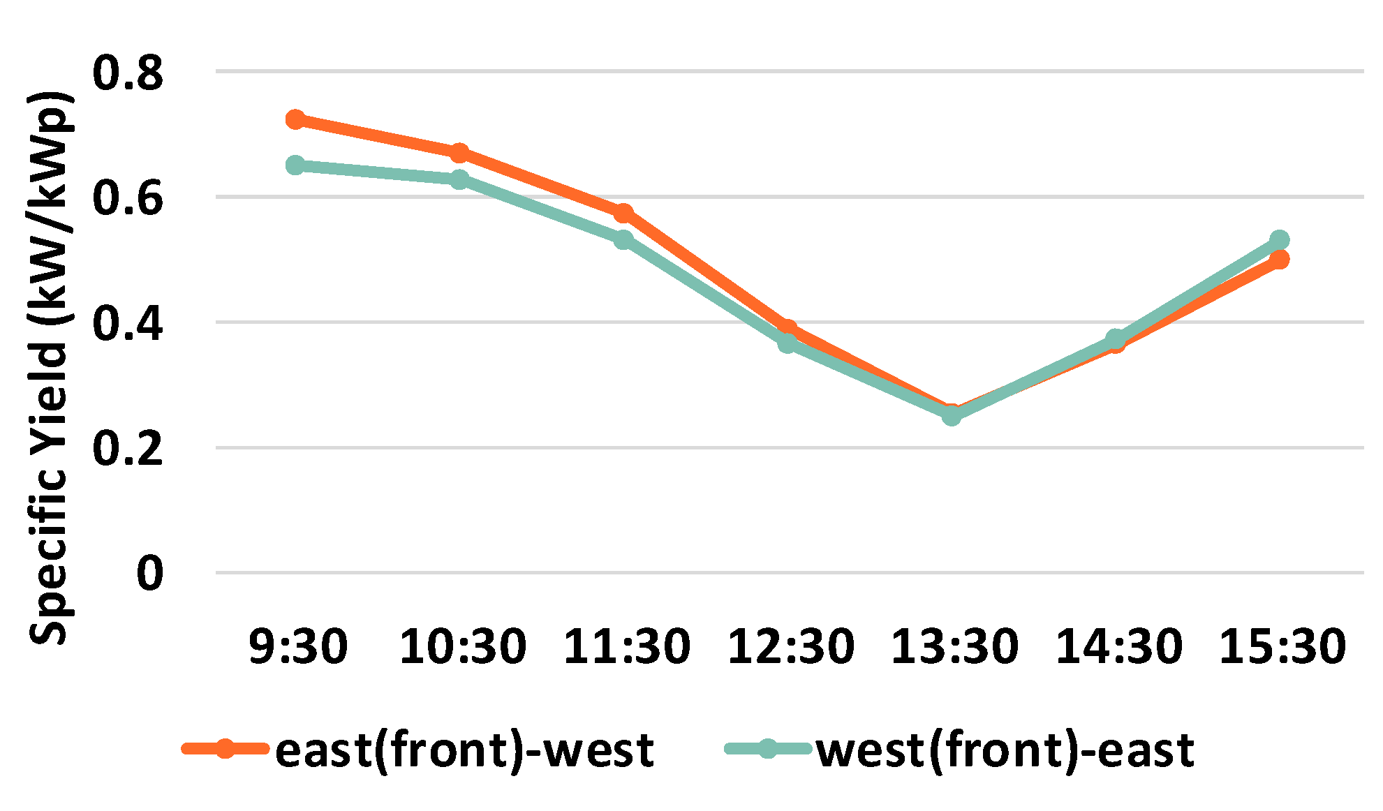
Figure 5.
I–V curve for the vertically set module at a specific time: (a) I–V curve for east (front)-west at 14:30 p.m.; (b) I–V curve for west (front)-east at 12:30 p.m.
Figure 5.
I–V curve for the vertically set module at a specific time: (a) I–V curve for east (front)-west at 14:30 p.m.; (b) I–V curve for west (front)-east at 12:30 p.m.

Figure 6.
Shadows on the rear surface at a specific time: (a) shadow on the rear-surface for the east (front)-west orientation at 14:30 p.m.; (b) shadow on the rear-surface for the west (front)-east orientation at 12:30 p.m.
Figure 6.
Shadows on the rear surface at a specific time: (a) shadow on the rear-surface for the east (front)-west orientation at 14:30 p.m.; (b) shadow on the rear-surface for the west (front)-east orientation at 12:30 p.m.

Figure 7.
Layout of the modules measured for temperature for Testbed 3: neighboring modules (modules no. 2 and no. 3) and distant modules (modules no. 2 and no. 8).
Figure 7.
Layout of the modules measured for temperature for Testbed 3: neighboring modules (modules no. 2 and no. 3) and distant modules (modules no. 2 and no. 8).

Figure 8.
Module surface temperature comparison for the modules in the summer and winter: (a) module surface temperatures on 6 August; (b) module surface temperature on 26 January.
Figure 8.
Module surface temperature comparison for the modules in the summer and winter: (a) module surface temperatures on 6 August; (b) module surface temperature on 26 January.

Figure 9.
Shadow locus for summer season (left) and winter season (right).

Figure 10.
Daily specific yield comparison for the modules in the summer and winter: (a) daily specific yield on 6 August; (b) daily specific yield on 26 January.
Figure 10.
Daily specific yield comparison for the modules in the summer and winter: (a) daily specific yield on 6 August; (b) daily specific yield on 26 January.
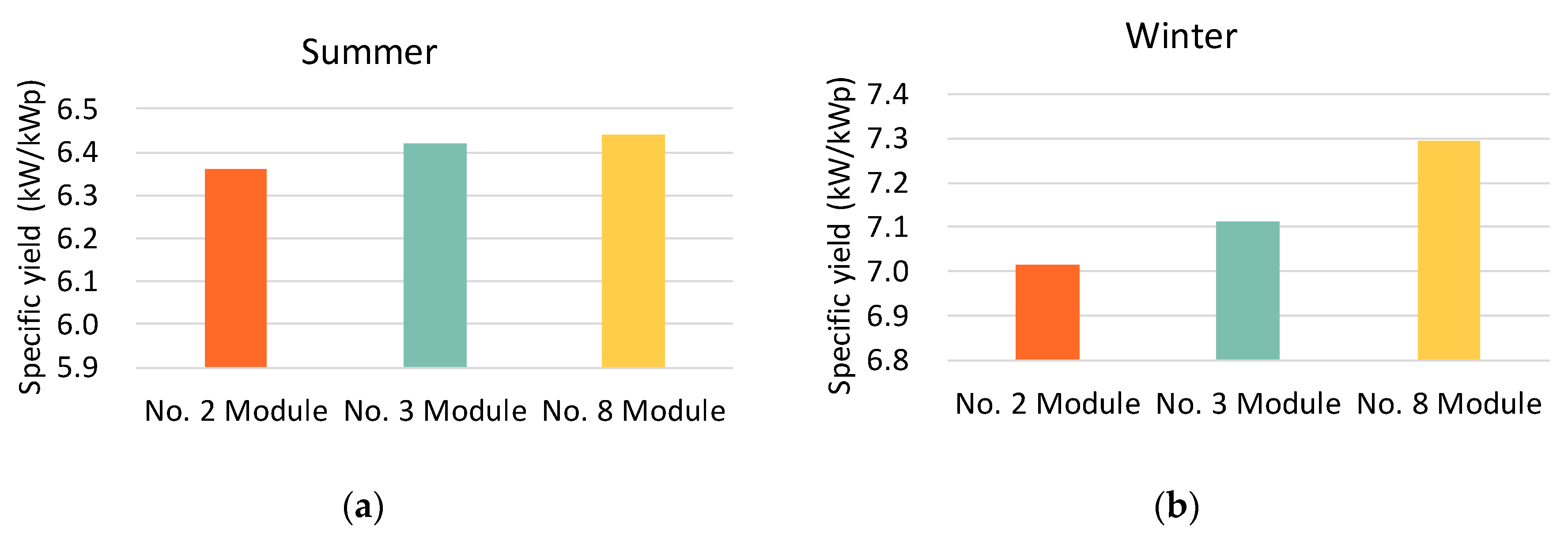
Figure 11.
Diffuse irradiance factor based on the concentration of particulate matter (PM): (a) clear sky; (b) overcast.
Figure 11.
Diffuse irradiance factor based on the concentration of particulate matter (PM): (a) clear sky; (b) overcast.

Figure 12.
Bifacial gain based on the concentration of PM: (a) clear sky; (b) overcast.


Table 1.
Installation conditions of testbeds.
| Testbed 1 | Testbed 2 | Testbed 3 | |
|---|---|---|---|
| Ground height | 1.4 m | 1.2 m | 1.5 m |
| Tilt angle | 37° | 90° | 37° |
| Azimuth angle | 0° (South) | −90° (East) to 90° (West) | 37° (South-West) |
| Albedo | 55% | 23% | 23%, 55% |
| Configuration | 1 series and 1 parallel | 1 series and 1 parallel | 8 series and 1 parallel |
Table 2.
Specification of the bifacial PV module at each testbed.
| Testbed | PV Module Parameter | Magnitude |
|---|---|---|
| Testbed 1 | Rated power (W) | 365 |
| Voltage at Pmax (V) | 39.7 | |
| Current at Pmax (A) | 9.19 | |
| Open-Circuit voltage (V) | 47.8 | |
| Short-Circuit current (A) | 9.66 | |
| Bifaciality factor (%) | 75 | |
| Type of module | P-PERC | |
| Testbed 2 and Testbed 3 | Rated power (W) | 285 |
| Voltage at Pmax (V) | 32 | |
| Current at Pmax (A) | 8.91 | |
| Open-circuit voltage (V) | 39 | |
| Short-circuit current (A) | 9.3 | |
| Bifaciality factor (%) | 82 | |
| Type of module | N-PERT |
Table 3.
Specification of the power conversion equipment at Testbed 3.
| Power Conversion Equipment | Parameter | Magnitude |
|---|---|---|
| DC Optimizer | MPPT operating range (V) | 8–60 |
| Nominal input DC power (W) | 370 | |
| Euro efficiency (%) | 98.8 | |
| Inverter | Maximum input voltage (V) | 480 |
| Nominal AC power (kW) | 3 | |
| Euro efficiency (%) | 98.8 |
Table 4.
Experiment categories.
| Testbed | Content | Configuration |
|---|---|---|
| Testbed 1 | Size of reflective material | 1 × 1 module |
| Testbed 2 | Vertical installation type | 1 × module |
| Testbed 3 | Position of modules in a row and concentration of PM | 8 × 1 modules |
Table 5.
Measurement equipment and items.
| Measurement Equipment | Measurement Items | Contents | |
|---|---|---|---|
| I–V checker (Kernel) |  | Pmax, Vmax, Imax, I–V curve | Section 3.1, Section 3.2 and Section 3.3 |
| IR camera (FLIR) |  | Module surface temperature | Section 3.3 |
| Data logger (solar edge) |  | Output power of module in the system | Section 3.4 |
| MS-80 (EKO) |  | Diffuse horizontal irradiance | Section 3.4 |
| LP PYRA 02 (OHM) |  | Global horizontal irradiance | Section 3.4 |
| SMPS (scanning mobility particle sizer) and OPC (optical particle counter) | - | PM 2.5, PM 10 | Section 3.4 |
Table 6.
Measured I–V curve data at a specific time.
| Time | Orientation | Isc (A) | Voc (V) | Imp (A) | Vmp (V) | Pmp (W) |
|---|---|---|---|---|---|---|
| 14:30 | east (front)-west | 3.708 | 37.38 | 3.189 | 33.13 | 105.65 |
| west (front)-east | 3.608 | 37.47 | 3.426 | 31.56 | 108.12 | |
| 12:30 | east (front)-west | 3.78 | 37.32 | 3.606 | 31.34 | 113.01 |
| west (front)-east | 3.753 | 37.21 | 3.207 | 32.92 | 105.57 |
Table 7.
Diffuse irradiance factor based on the concentration of PM at specific points.
| PM 2.5 | PM 10 | |||
|---|---|---|---|---|
| 0 µg/m3 | 150 µg/m3 | 0 µg/m3 | 100 µg/m3 | |
| Clear sky | 19.77% | 57.27% | 18.27% | 34.27% |
| Overcast | 95.7% | 101.7% | 98.68% | 96.68% |
Table 8.
Bifacial gain based on the concentration of PM at specific points.
| PM 2.5 | PM 10 | |||
|---|---|---|---|---|
| 0 µg/m3 | 150 µg/m3 | 0 µg/m3 | 100 µg/m3 | |
| Clear sky | 32.01% | 38.1% | 31.03% | 35.03% |
| Overcast | 50.16% | 50.91% | 51.2% | 50.3% |
© 2020 by the authors. Licensee MDPI, Basel, Switzerland. This article is an open access article distributed under the terms and conditions of the Creative Commons Attribution (CC BY) license (http://creativecommons.org/licenses/by/4.0/).
Share and Cite
MDPI and ACS Style
Jang, J.; Lee, K. Practical Performance Analysis of a Bifacial PV Module and System. Energies 2020, 13, 4389. https://doi.org/10.3390/en13174389
AMA Style
Jang J, Lee K. Practical Performance Analysis of a Bifacial PV Module and System. Energies. 2020; 13(17):4389. https://doi.org/10.3390/en13174389
Chicago/Turabian StyleJang, Juhee, and Kyungsoo Lee. 2020. "Practical Performance Analysis of a Bifacial PV Module and System" Energies 13, no. 17: 4389. https://doi.org/10.3390/en13174389
Note that from the first issue of 2016, this journal uses article numbers instead of page numbers. See further details here.