Recursive Feature Elimination and Random Forest Classification of Natura 2000 Grasslands in Lowland River Valleys of Poland Based on Airborne Hyperspectral and LiDAR Data Fusion

Abstract

The use of hyperspectral (HS) and LiDAR acquisitions has a great potential to enhance mapping and monitoring practices of endangered grasslands habitats, beyond conventional botanical field surveys. In this study we assess the potentiality of recursive feature elimination (RFE) in combination with random forest (RF) classification in extracting the main HS and LiDAR features needed to map selected Natura 2000 grasslands along Polish lowland river valleys, in particular alluvial meadows 6440, lowland hay meadows 6510, and xeric and calcareous grasslands 6120. We developed an automated RFE-RF system capable to combine the potentials of both techniques and applied it to multiple acquisitions. Several LiDAR-based products and different spectral indices (SI) were computed and used as input in the system, with the aim of shedding light on the best-to-use features. Results showed a remarkable increase in classification accuracy when LiDAR and SI products are added to the HS dataset, strengthening in particular the importance of employing LiDAR in combination with HS. Using only the 24 optimal features selection generalized over the three study areas, strongly linked to the highly heterogeneous characteristics of the habitats and landscapes investigated, it was possible to achieve rather high classification results (K around 0.7–0.77 and habitats F1 accuracy around 0.8–0.85), indicating that the selected Natura 2000 meadows and dry grasslands habitats can be automatically mapped by airborne HS and LiDAR data. Similar approaches might be considered for future monitoring activities in the context of habitats protection and conservation.

1. Introduction

Protecting and monitoring natural habitats is essential for the mitigation of biodiversity decline, caused by the negative effects of increased human activity [1] and the natural adaptation to climate change. Back in 1992, the European Union established the Habitats Directive [2], a cornerstone European nature conservation policy, developing the wide Natura 2000 ecological network of protected areas with the aim of preserving the most valuable sites in the European landscape. Within the Natura 2000 habitats, grasslands are one of the most biodiverse habitats in Europe [3], delivering essential ecosystem services for our societies [4]. These habitats are important because of the preservation of natural values occurring in the agricultural landscape of lowland river floodplains, including fauna and flora species strictly connected with periodic floods and with extensively used agricultural habitats, as meadows and/or pastures [5,6]. River valleys, with a properly developed structure of natural habitats, perform important ecological functions as ecological corridors, including for migratory species [7,8,9]. The diverse, mosaic structure of the natural habitats of river valleys is conducive to both maintaining and restoring biodiversity and strengthening ecosystem services [10,11,12]. Thus, it is crucial to maintain this original, natural structure in good condition.

Semi-natural, non-forested ecosystems have been managed by grazing and mowing for centuries [13]. However, changes in the agricultural land use, mainly related to the recent intensification of agricultural production, have caused a major decline in the biodiversity of natural and semi-natural ecosystems located in river valleys [14]. Currently, they are also threatened and often replaced by plant communities of lower light requirements due to land abandonment, inducing process of spontaneous secondary succession. In the context of progressive climate changes, plant communities developing in river valleys and its state may be used as an indicator of transformation of water-dependent ecosystems into those that do not require permanent or periodic high soil humidity [15,16]. In Poland, in the lowland river floodplains, there are a number of valuable natural habitats, classified with specific codes according to the Habitats Directive [2]. The most important are: 3270-muddy banks rivers with Chenopodion rubri and Bidention vegetation, 6440-alluvial meadows in river valleys of the Cnidion dubii, 6410-Molinia meadows on calcareous, peaty or clayey-silt-laden soils (Molinion caeruleae), 6510-lowland hay meadows (Alopecurus pratensis, Sanguisorba officinalis), 6120-xeric sand calcareous grasslands (Koelerion glaucae), 91E0-alluvial forests with Alnus glutinosa and Fraxinus excelsior (Alno-Padion, Alnion incanae, Salicion albae).

With their biodiversity, habitats 6440, 6510, and 6120, belong to relatively poorly known and at the same time disappearing landscape elements in the territory [17], mostly due to changes caused by anthropic pressure. Therefore, it is important to have updated, precise and reliable spatial information for the monitoring and characterization of these habitats. Every six years, Member States are requested to provide a monitoring report on the status and development of their Natura 2000 sites [2]. Most of these monitoring activities consist in field-botanical surveys, conducted in specific and limited research areas, where the natural habitats occur [18]. The problem of such monitoring approach is the operator-related subjectivity and the relatively small number of habitat patches that can be surveyed, due to the high time-consuming efforts needed and the difficulty to reach inaccessible remote areas [19].

The waves of scientific-technological innovations that characterized the latter half of the 20^th century [20], yielded a new generation of remote sensing (RS) technologies that has changed the way we can analyze and monitor our environment [21,22]. The possibility of having access to higher spatial and spectral resolution RS data, covering ever larger areas, offers a wealth of novel opportunities to enhance modern environmental monitoring and management [23,24]. Indeed, data collected by RS platforms are more robust with respect to discontinuous field-based information because they rely on continuous and quantitative information that can be repeated through time, making their assessment not only more time- and cost-effective, but also more objective and less influenced by human’s subjectivity [25,26].

In recent years, different RS technologies have been exploited more consistently for mapping and monitoring Natura 2000 habitats [27], although the number of studies focusing on grasslands mapping are relatively low as compared to other types of habitats [28]. Multi-temporal high resolution RapidEye satellite data have been used to develop a large-scale assessment of grassland use intensity in southern Germany [29]. Certain types of grassland habitats have been classified using intra-annual time series analysis, achieving similar accuracies with either RapidEye or TerraSAR-X data [30]. Object-based analysis has also been employed when analyzing WorldView-2 very high spatial resolution satellite data [31].

The recent enhancements in the spectral and spatial resolution of sensors have enabled the development of new opportunities for a wider application of hyperspectral imaging (HS) in environmental monitoring [32]. Characterized by both high spatial and spectral resolution, they typically record the reflected object’s light across hundreds of narrow spectral bands, within the visible, near infrared (NIR), mid infrared (MIR), and short-wave infrared (SWIR) parts of the electromagnetic spectrum [33,34], resulting in a 3-dimensional hyperspectral data-cube [35]. More and more studies have recently focused on exploiting this wealth of spectral information for natural habitats mapping [19,36]. For example, few works have been found in the current literature focusing on the exploitation of HS potentials for heathland habitats mapping and conservation, using different techniques such as, spectral unmixing [37], machine learning classification [38], or object-based image analysis [39,40].

In recent years, it has also been proven and recognized that light detection and ranging (LiDAR) systems, also referred to as airborne laser scanning (ALS), are a good alternative for vegetation mapping and characterization [41,42,43,44,45]. Some studies have shown how the combination of ALS with HS data can enhance the accuracy of habitats mapping [46,47,48,49], emphasizing the importance of simultaneously exploiting both the spectral and topographical information when targeting the automatic identification of such types of natural habitats [50]. However, the effective fusion of the two complementary data sources is a challenging task. The high dimensionality of the data and the limited availability of ground-truth samples, especially when it comes to natural habitats mapping and characterization, pose major challenges in data handling and processing [51,52]. The first one, also referred to as the curse of dimensionality [53], can be addressed by using dimensionality reduction methods [54], supposed to remove redundant data without losing original and relevant information. Among these techniques, the feature-selection based approaches, whose objective is to find a subset of the relevant data from the original dataset, are reported to be simpler, easier to implement, and very efficient at the same time [55,56,57]. The future-selection methods are also reported to be effective methods in handling the fusion of diverse data sources, such as HS and LiDAR data, as they allow to consider all available information simultaneously in a decision-making system in which the different sensor data can be selected [58]. In the last years, several investigators have carried out research in this specific field, combining the feature-selection capabilities with machine learning (ML) classification [52,59,60,61], for a broad range of applications [62,63,64]. Among these techniques, it has been highlighted by several authors that recursive feature elimination (RFE) combined with random forest (RF) classification could provide unbiased and stable results in different application fields [65,66,67,68]. However, to our knowledge, this method was not investigated yet for mapping meadows and dry grasslands.

The main objective of this study is thus to assess the performances of RFE-RF for integrating airborne hyperspectral and LiDAR data in the context of mapping selected Natura 2000 habitats found along Polish river valleys; in particular, alluvial meadows (6440), lowland hay meadows (6510), and xeric and calcareous grasslands (6120). With this work, we aim at identifying the main features required to automatically classify these habitats and at the same time emphasizing the added value of the fusion between such complementary and diverse datasets.

Airborne flight campaigns with HS and LiDAR sensors were conducted simultaneously to botanical field-surveys three times in the growing seasons (Spring/Summer/Autumn), along three significative river valleys in Poland, with a good distribution of lowland meadows and dry grasslands habitats, as described in Section 3.1. With the aim of combining the RFE method with RF classification, an RFE-RF automated classification system was developed and is described in Section 3.4. Three different experiments were designed in line with the objectives of this paper, as described in Section 3.5. In the first one, we aimed at identifying the relevant spectral features for meadows and dry grasslands mapping, by applying the RFE on the hyperspectral dataset alone and comparing results with a standard, well-known dimensionality reduction technique, the minimum noise fraction transformation (MNF) [69,70,71,72]. The most effective method for hyperspectral dimensionality reduction was then retained for the second experiment, in which several spectral- and topographical-based metrics were computed and added to the RFE-RF classification system. Using the RFE technique, we derived for each case study, a list of optimal features selection which might represent the best-to-use features for the investigated classification problem. In the third experiment, as a sort of verification test, only the best-to-use selected features were used to run the final classification maps. In this way, we could attempt to generalize a best-to-use features selection to be calculated from ALS and HS data respectively, for the classification of the selected Natura 2000 grasslands (6440, 6510 and 6120) in the analyzed river valleys.

2. Study Areas and Botanical Description

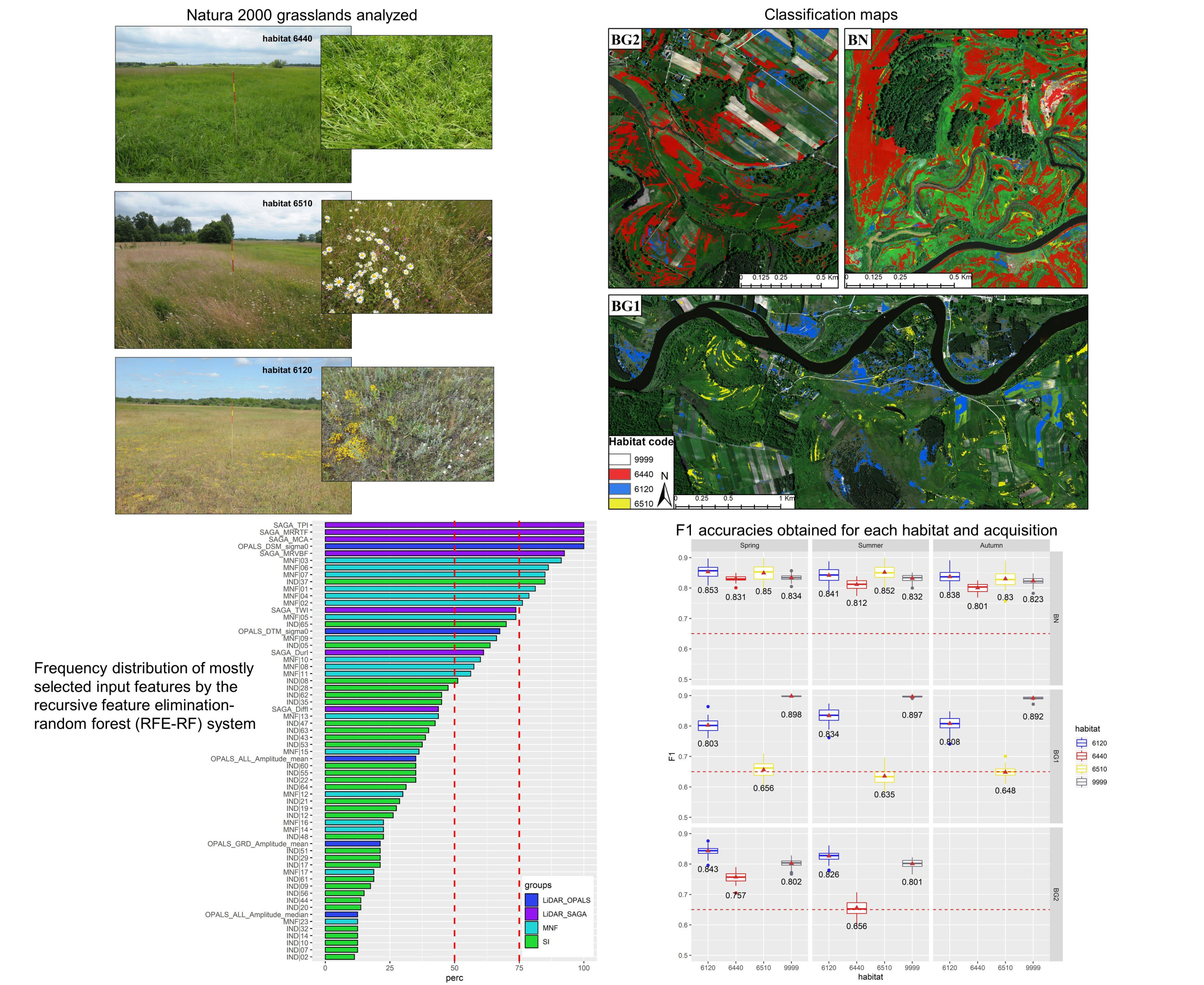
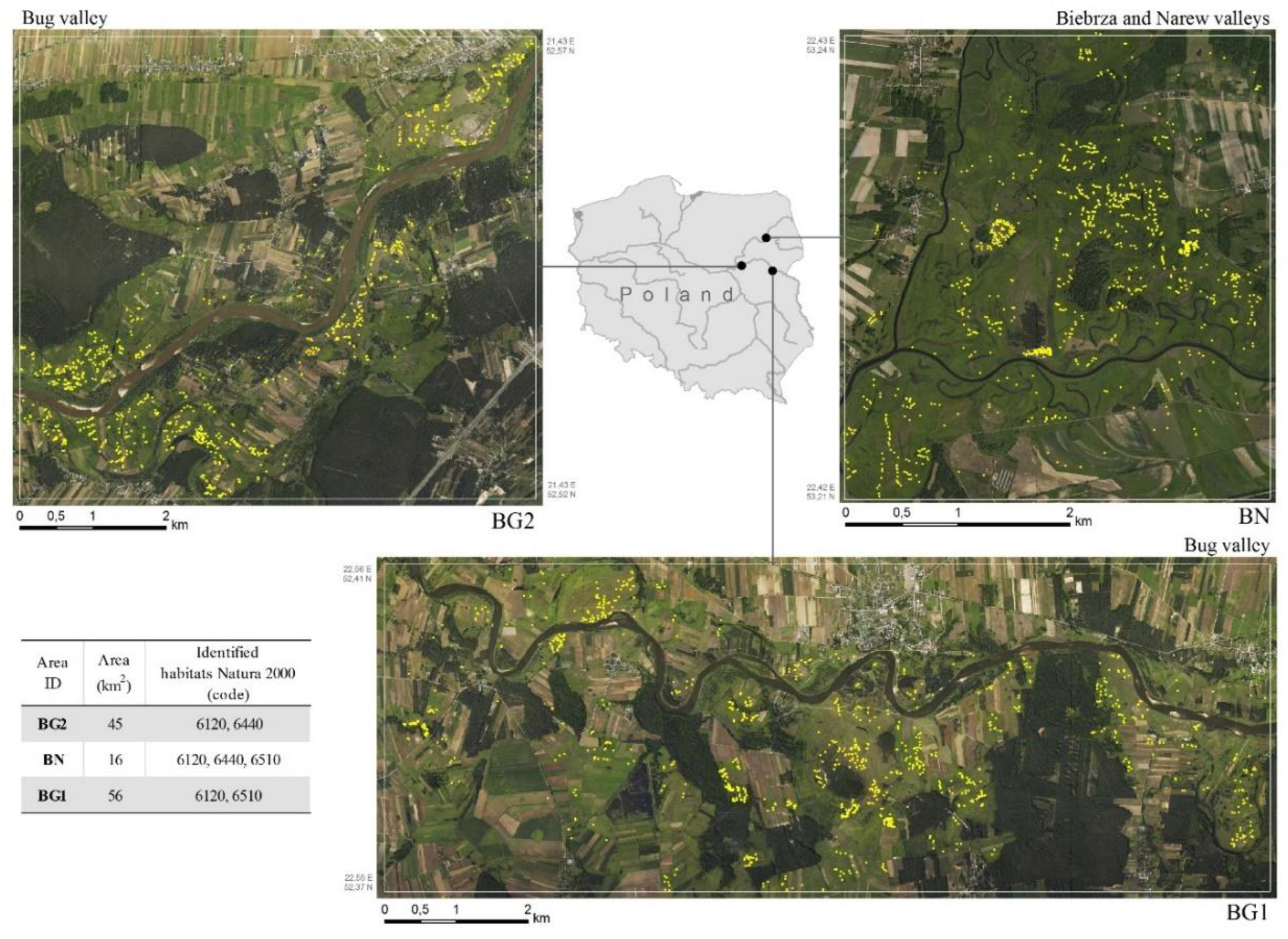
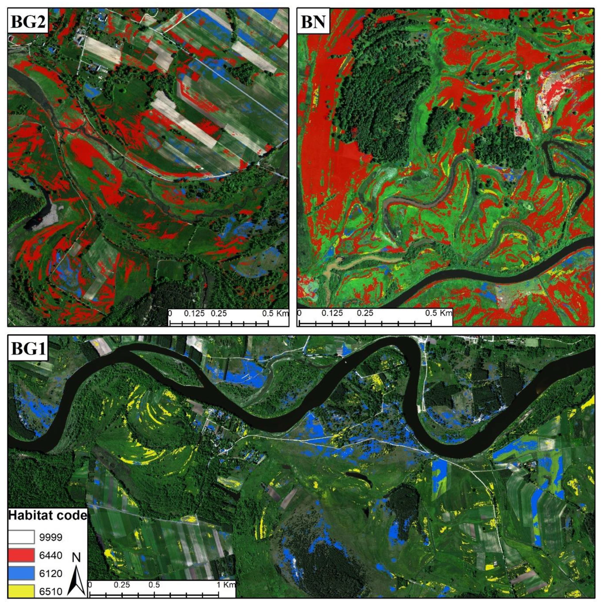
2.1. Study Areas

The research study areas are located in chosen lowland river valleys in Poland (part of the North European lowland), on sections characterized by the presence of well-developed semi-natural, open Natura 2000 natural habitats (in particular habitats 6440, 6510 and 6120).

The BN study area is approximately 16 km² (Figure 1), covering the estuary of the Biebrza and Narew rivers and its floodplain, in the northeast of the country. On the floodplain there is a varied fluvial microrelief, visible on the digital terrain models (DTM) computed from the ALS flights (Figure 2). The characteristic elements are: flat-bottomed depressions, narrow longitudinal depressions of overgrowing old river beds, flat elevations, small longitudinal elevations of old river bars, natural levees, as well as remnants of higher terrace levels (with traces of aeolian process) [73]. The floodplain is dominated by mineral and organic-mineral deposits, and also other organic materials, such as mud. Higher terrace levels are made of sandy and sandy-silty formations. The development of natural habitats in both valleys is influenced by the system of embankments and dikes extending both along the Biebrza (limiting the floodplain from the west) and Narew rivers (the embankment located south of the riverbed).

The study areas in the Bug river valley represent two sections of the river (BG1, BG2, Figure 1), typical for the middle and lower course, with a total area of about 100 km². Both sections of the valley are characterized by a highly diverse fluvial microrelief (Figure 2), with fragments of flat flood-basin and upper terraces, longitudinal, narrow depressions of oxbow lakes, natural levees, extensive flat-bottomed depressions on the floodplain, as well as longitudinal and narrow raised berms or crests above the floodplain surface [74]. The soil cover is definitely dominated by alluvial soils developed on sandy and sandy-silty formations, locally showing traces of aeolian processes.

The selected study areas have in common a highly variable topographical micro-relief (as described above and highlighted in Figure 2), a typical condition for the development of the investigated Natura 2000 habitats. In such highly variable topographical context, the extraction of LiDAR-based metrics could be very meaningful and is expected to bring a significant contribution to the quality of the classification results.

2.2. Natura 2000 Habitats Descriptions

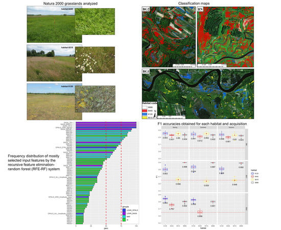
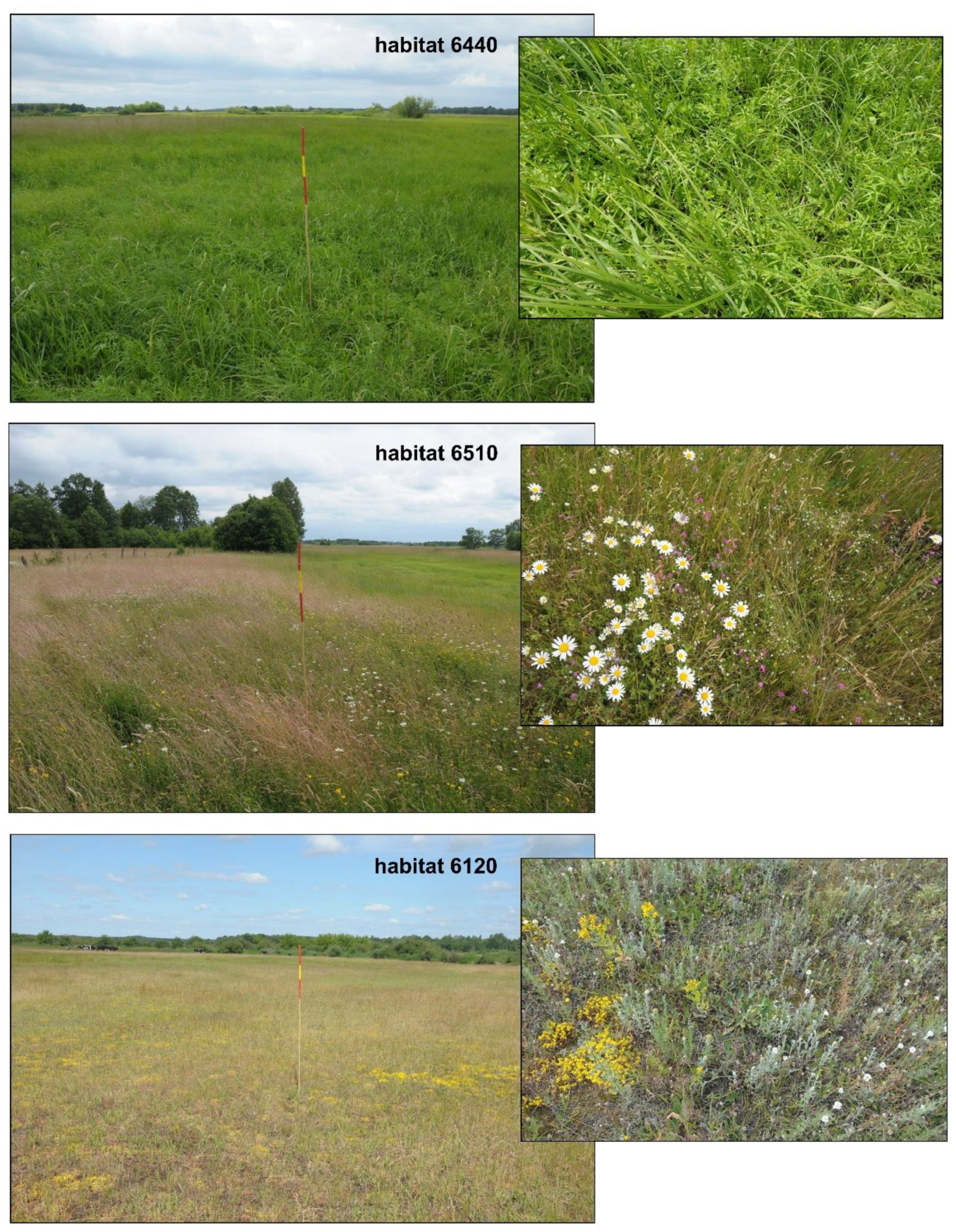
2.2.1. Habitat 6440: Alluvial Meadows of River Valleys of the Cnidion Dubii

Alluvial meadows of river valleys of the Cnidion dubii are semi-natural, fertile communities, usually mown twice, in Poland associated with the floodplains of main rivers. They arise in places where flooding or inundation occurs periodically [5]. Thus, they are adapted to changing moisture conditions, and are usually spotted in shallow depressions, on fertile, soils, on the slopes of alluvial forms or on slightly elevated flat parts of the plain built of sandy or silty material. They show high variability in species composition [75,76]. In addition to the characteristic and distinctive plant species (e.g., Cnidium dubium, Allium angulosum, Scutellaria hastifolia, Viola stagnina, and Gratiola officinalis), it may occur species that require higher moisture content, as well as those that are typically associated with dry habitats. The main current threats include no periodic flooding, too intensive agricultural use, or abandonment of landuse [77,78]. Habitat occurs in both chosen case studies for this research. In the Biebrza and Narew valleys (BN), habitat 6440 is commonly associated with flat-bottomed, extensive and shallow depressions (Figure 3). In the sections of the Bug valley (BG1 and BG2), it occurs less frequently and it is related mostly to narrow depressions of former oxbows or longitudinal and narrow raised berms or crests.

2.2.2. Habitat 6510: Lowland Hay Meadows

Lowland hay meadows are semi-natural communities where hay is most often obtained twice a year. They originated on fertile mineral soils in various morphological conditions and because of long-term not intensive agricultural use [5,79]. The habitat is composed of plant communities which arise in river valleys on upper terraces—beyond the extends of floods and inundation [80]. The lowland hay meadows are considered as one of the richest in plant species, hosting numerous fauna (mainly invertebrates) and being highly variable in terms of physiognomy [79], but at the same time at high risk of transformation into arable fields [79]. The most often observed characteristic plant species of the habitat are: Galium mollugo, Campanula patula, Knautia arvensis, Rumex thyrsiflorus. Because of the lack of typically shaped upper terraces, as well as the light sandy alluvial deposits, patches of habitat in the analyzed section of the BN valley are rare and scattered. They are found on the few flat elevations of the floodplain, where they form intermediate plant communities, with a large share of species typical of dry grassland habitats (Figure 3). In the Bug valley, lowland hay meadows occur in BG1 at upper terraces, which are not transformed into intensively used meadows or arable fields.

2.2.3. Habitat 6120: Xeric and Calcareous Grasslands

Xeric sand calcareous grasslands are semi-natural plant communities that have originated as a result of extensive grazing of grasslands on permeable, relatively fertile, and sandy soils. Thus, they occur in different landscape types [81] but very often in Poland are spotted in river valleys on extensive flat elevations outside the flood extends. The plant cover is loose, and besides grass species (e.g.,: Koeleria glauca, Festuca polesica, Corynephorus canescens), it contains numerous herbaceous plants (e.g.,: Silene otites, Silene tatarica, Astragalus arenarius, Kochia laniflora), as well as moss-lichen layer [5,82]. Plant communities of dry grasslands in Poland show great diversity and dynamics resulting from landuse, soil and geographical conditions that affect the species composition, and sward density. Currently the most serious threats are related to land abandonment, lack of regular grazing, and overgrowing by shrubs. In the analyzed section of the BN valley, habitat 6120 occurs on small areas (up to 100 m²), and is associated with distinct sandy elevations. Dry grasslands in the Bug valley are definitely more widespread and more typically developed (Figure 3).

3. Methodology

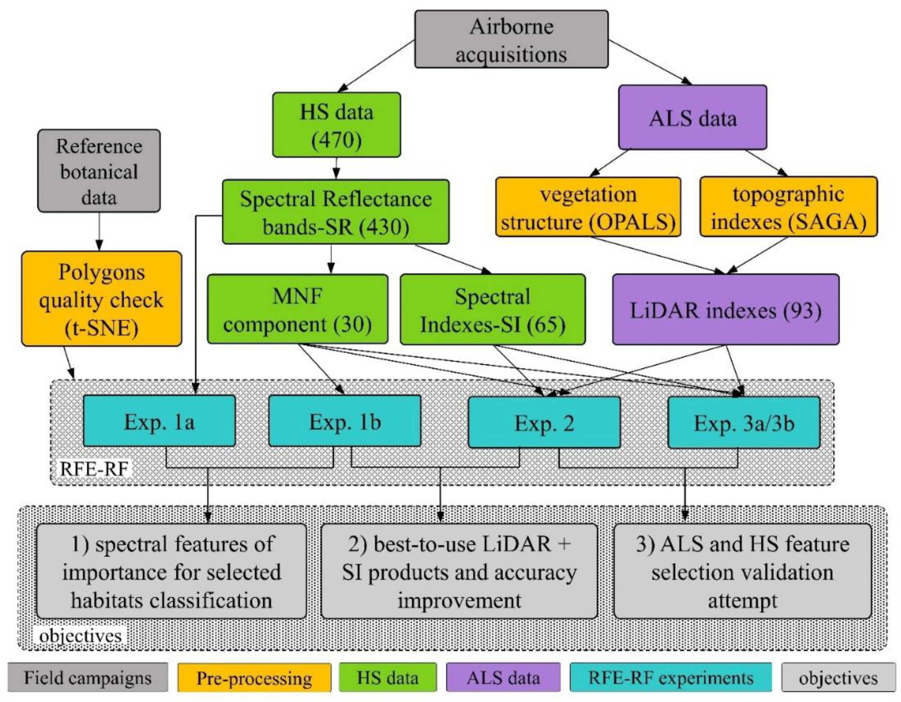
3.1. Airborne Data Acquisition and Botanical Field Measurements

Airborne flight campaigns and botanical field data were acquired simultaneously three times in the growing season (Spring/Summer/Autumn). The campaign dates were chosen taking into account the phenological period and agricultural practices. Thus, the optimal terms for obtaining aerial photographs and conducting field survey were planned at the end of May, the middle of July and the beginning of September. The RS flight campaigns were conducted during the best possible weather conditions, using RS platform with the following sensors installed:

• Hyperspectral scanners (Hyspex: VNIR 0.4–0.9 µm & SWIR 0.9–2.5 µm): 470 spectral bands with 1 m spatial resolution;
• Airborne Laser Scanner (Riegl Lite Mapper LMS-Q680i): point cloud data acquired with 7 points/m²;
• Medium format RGB camera (50Mpix) with 0.1 m spatial resolution.

For more technical details about the RS platform, the reader is referred to [83]. Field spectro-radiometric measurements were also taken in the field with ASD FieldSpec 4, at selected bright and dark locations to be used in the later stage for atmospheric correction (Section 3.2).

An extensive campaign of botanical surveys was conducted by teams of specialized botanists, according to a uniform procedure worked out within the HabitARS project (Habitats Airborne Remote Sensing) [83,84,85]. Botanical research did not last more than seven days from the date of airborne flight campaigns. The procedure for obtaining botanical reference material involved several stages. At the stage of the preliminary reconnaissance, the area was analyzed because of the diversity of natural habitats (based on available data) and to the spatial distribution of habitat patches. Once recognized, GPS points were recorded using a GPS receiver of 0.5 m accuracy. Reference polygons of 3-m radius were established at locations typical and representative for the particular habitat in the research area, homogenous due to vegetation type and structure of plant community, without physical disturbances caused by animals (e.g., wild boars), agricultural machinery etc. Reference polygons did not encompass trees and shrubs higher than 1.5 m, and were also located at a distance from high elements (e.g., trees, escarpments) in order to avoid shadows. For each reference polygon, a standard description of vegetation and applied agricultural practices was performed. The botanical surveys were also supplemented by photographic documentation and in a later stage were organized into a GIS-database. The same procedure was repeated for as many patches of habitats 6120, 6440, and 6510 as possible, in order to have a good spatial distribution of samples (Figure 1). Other GPS points were also collected in vegetation patches not considered to be a habitat or representing other land-cover classes and were assigned to the background class (code 9999).

3.2. Reference Botanical Data Quality Assessment

The quality of field reference dataset is a crucial aspect that must be considered carefully because it strongly influences the quality of classification results [86,87], especially in highly heterogeneous plant communities. Moreover, because of the non-simultaneity of some field measurements with respect to airborne acquisitions and to the fact that these natural areas are affected by mowing, an appropriate selection and quality assessment procedure was implemented before using the reference dataset for automatic classification.

The first step of this procedure was the visual recognition with the simultaneously acquired RGB-aerial photographs, in order to eliminate defective/erroneous reference polygons. Polygons were removed from the reference set when on the given RGB mosaic they were: mowed, in shadow, inundated, mechanically damaged (by animals or farming), or had other problems. In the second step, a cleaning of the dataset was performed using the t-distributed stochastic neighbor-embedding (t-SNE) algorithm [88]. In a recent study, it has been demonstrated that the t-SNE algorithm is able to increase the final classification accuracy of 6% in Kappa coefficient [85]. This algorithm was created to efficiently visualize high-dimensional data in order to understand the underlying spectral relations between groups of points. Each multidimensional polygon can be plotted in a two-dimensional space, as showed in Figure 4. Points which are close to each other share similar remotely sensed (spectral) features, while different samples are represented by distant points. In this way, a multi-dimensional dataset can be interpreted in an easier way, revealing its global structure, such as the presence of clusters and their spectral characteristics.

In this study, t-SNE algorithm was used to evaluate if reference polygons were correctly assigned to the belonging habitat class [85]. A series of iterative visualizations, with perplexity hyper-parameter varying between 5 and 130, were performed. PCA-based initialization was used to provide stable global layouts. Figure 4 presents the t-SNE plots using a perplexity value of 30 and after removal of detected incorrect points, for all areas and acquisitions analyzed. It depicts the real spectral characteristics of the investigated habitats. Habitats 6120 and 6440 are clearly clustered and it seems that they hold quite different spectral characteristics among both BN and BG2 areas. Instead, habitat 6510 seems slightly more mixed with other classes, being in-between habitats 6120 and 6440 in BN-related plots. However, if we compare habitat 6510 only to habitat 6120 in BG1-related plots, it seems they have more clear differences. Over all plots, the background class (code 9999) is the one having the highest heterogenous spectral characteristics.

The final numbers of reference polygons, obtained after the quality assessment and used for classification, are shown in

Table 1. Number of reference polygons for each habitat class and study area.

		Habitat Class
Area	Acquisition	6120	6440	6510	Background (9999)	Total
BN	Spring	144	492	105	722	1463
	Summer	146	376	111	619	1252
	Autumn	141	315	74	550	1080
BG1	Spring	191	-	235	1036	1462
	Summer	180	-	193	917	1290
	Autumn	192	-	249	996	1437
BG2	Spring	272	289	-	587	1148
	Summer	268	224	-	586	1078

for each habitat and study area analyzed. The higher number of background polygons (class 9999) is justified by the large acquisition areas (such as BG1) and therefore by the much higher spatial distribution of heterogeneous non-habitat classes.

3.3. RS Data Pre-Processing

In Figure 5 a scheme of the pre-processing steps is illustrated, together with the experiments design (Section 3.5) and the corresponding addressed objectives in the paper. The HS images were radiometrically and geometrically corrected with the PARGE software [89] and atmospherically corrected using ATCOR4 model [90], using as a verification the ASD field spectral measurements collected at several locations. The result of each acquisition was a mosaicked orthophoto at 1-m resolution, with 430 spectral reflectance bands (SR) in the range 450–2500 nm. Several spectral indices (SI) were calculated using the ENVI 5.3 software. The reader is referred to the ENVI’s user guide [91] for a detailed listing of all 65 SI computed for this study. The minimum noise fraction transformation (MNF), a well-known technique for hyperspectral dimensionality reduction and denoising, was also computed for each image [69]. Based on eigenvalues and after testing with different number of bands, we decided to retain the first 30 MNF components, also as suggested in other studies [83]. From the ALS acquisition, 93 LiDAR-based indices were computed after point-cloud pre-processing. They consisted of vegetation structure layers, extracted from the OPALS software [92], and of topographic indices extracted from the SAGA software [93]. All produced rasters were re-projected with final spatial resolution of 1 m. The different RS-based products generated in this phase were then used as an input in the different classification experiments using the RFE-RF system, as depicted in Figure 5 and explained in detail in Section 3.5.

3.4. Recursive Feature Elimination-Random Forest (RFE-RF) Classification System

The RFE is a feature selection method that aims at estimating which features are most helpful to discriminate the classes of interest. It is able to eliminate any features that are not useful in this task, in order to obtain the input feature-set having the lowest possible number of layers, at the same time without reducing the final classification accuracy. The algorithm relies on variable importance assessment, which is calculated internally by RF classifiers and requires performing multiple rounds of classification. Each round consists of learning a new RF classification model, assessing its accuracy based on cross-validation, analyzing the feature of importance metrics for every feature used, and modifying the feature-set that would be used for the successive round of the procedure. The first classification round is performed using all the available features. Then, the weakest performing ones are detected using variable of importance metric, estimated by the model during learning. One (or more) of the weakest features are then eliminated from the feature-set, and the next round of the procedure is performed. By doing so, RFE attempts as well to eliminate dependencies and collinearity that may exist in the input features.

One of the objectives of this paper is to develop an RFE-RF system, capable of combining the potentiality of RF classification and RFE feature selection, at the same time automatizing the analysis of HS and LiDAR data for our habitats mapping purpose. A vegetation classification studio (VCS) software was therefore developed [94], based on RF classification and RFE dimensionality reduction technique. The VCS software reads simple text-language commands defined by users, which allow the automatization of the whole RF classification procedure, such as splitting reference data into training/validation sets, model training and validation, feature selection with RFE, accuracy assessment and plotting classification maps results, where needed. In this way, multiple classification cycles can be easily defined and automated, bringing more confidence to the results, since based on numerous experiments and not just a few. Moreover, the performing efficiency in terms of processing time needed to generate classification maps, after the preparation of the input and reference data (described in Section 3.2 and Section 3.3), is much higher than other non-automated systems.

When the RFE option is used in the VCS software, an RFE report is produced in the results (Figure 6). This is employed in the next step for the definition of the optimal feature selection to be chosen as the best-to-use feature configuration out of the multiple run sequences, generally being the one having the best compromise in terms of higher Kappa and lower number of features. Figure 6a illustrates the different classification results sorted by classification run sequences (on the x-axis). If the same results are sorted by the Kappa values (Figure 6b), it is possible to locate the point where a major increase in the number of features (green line, fc) will not cause a major change in the Kappa results. In this example, run 100 produced a Kappa of 0.631 using 23 features, while a similar Kappa value of 0.632 was obtained using 430 features. Therefore, run 100 can be retained as the optimal feature selection because by using a much lower number of features a very similar Kappa accuracy can be achieved.

3.5. Experiments Design

The different experiments described below and resumed in

Table 2. Different experiments’ characteristics.

Objective	Objective	Input features	RFE	Feature nr.	Runs	Training/Validation Sampling
1a	Spectral features of importance for selected habitats classification	SR	yes	430	10	50/50, random manual selection
1b		MNF	no	30	10	50/50, random manual selection
2	Best-to-use HS + ALS products and accuracy improvement	MNF + LiDAR + SI	yes	188	10	50/50, random manual selection
3a	Feature selection validation attempt	Area-dependent selection	no	24-28	50	50/50, random automatic selection
3b		Common selection	no	24	50	50/50, random automatic selection

were designed with the aim of addressing the objectives set out for this paper.

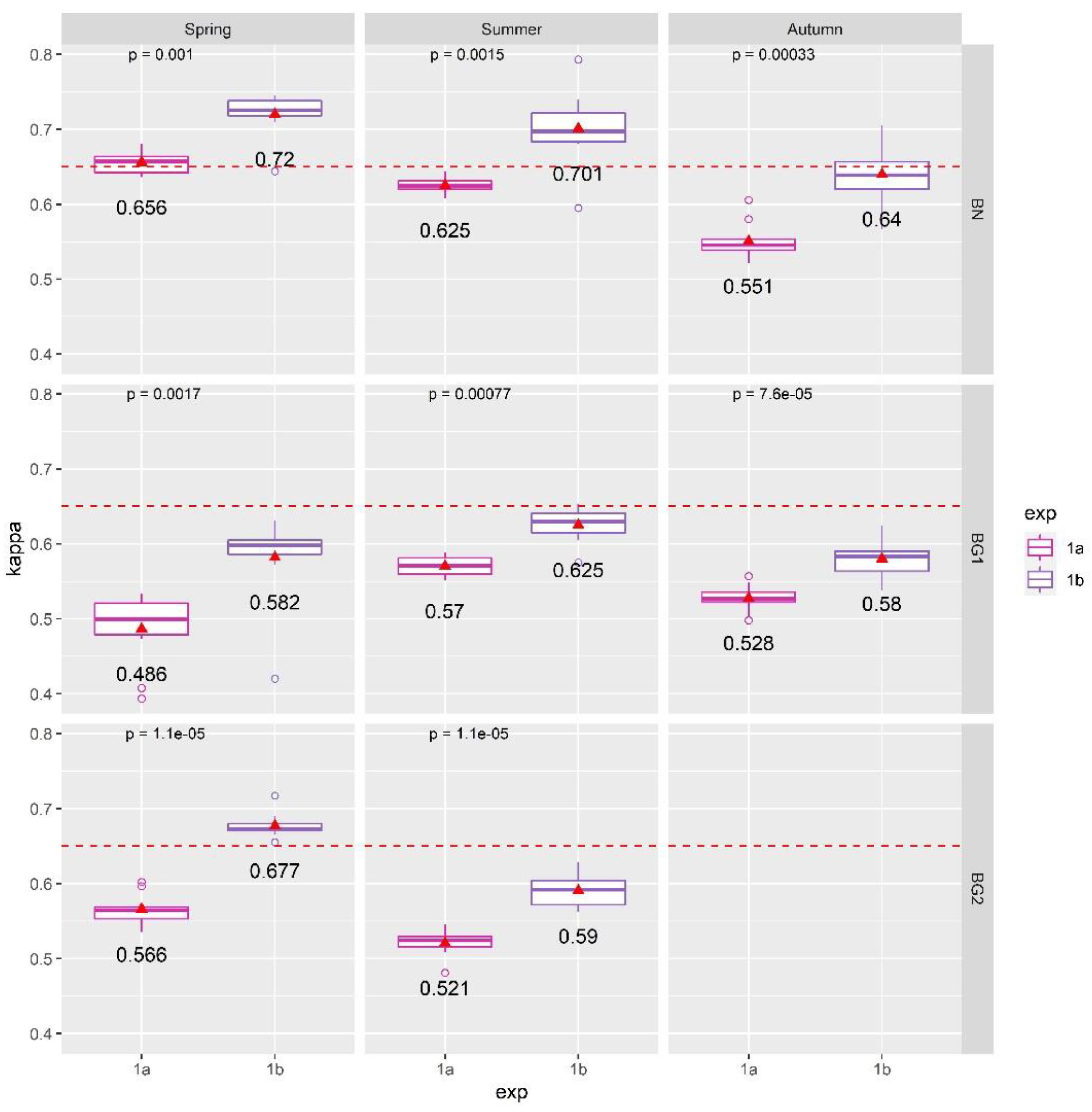
3.5.1. Exp. 1: Spectral Features of Importance and Dimensionality Reduction

One of the objectives of this paper is to understand which spectral features are more important for automatic classification of selected meadows and dry grasslands habitats and which dimensionality reduction technique is most effective. For this reason, the RFE technique was compared to the well-established data transformation technique MNF. The 430 SR bands were compared to the 30 MNF components, by running two different experiments (Figure 5). In the first experiment (Exp. 1a), only the 430 SR bands were analyzed. The RFE technique was used together with RF classification (RFE-RF), in order to identify which spectral bands are mostly used for the classification of the investigated habitats (see also Table 2). In the second experiment (Exp. 1b), only the 30 MNF components were used for RF classification and without the RFE option. In both cases (Exp. 1a/1b), selection of samples was done manually on a 50/50 basis: ten different random sample selections were manually realized and ten different shapefiles produced for the classification (Table 2). In this way, instead of using just one training/validation selection, ten different RF classification runs were realized and a better statistical distribution of both Kappa accuracy and optimal spectral features selection will be possible. The aim was to analyze the lists of optimal features selections among the ten different runs and then finding a certain number of commonly selected HS channels, which might represent the spectral features of importance for the habitats 6120, 6440, and 6510. The dimensionality reduction technique producing the highest classification results was then retained and used for the next experiment (Exp. 2).

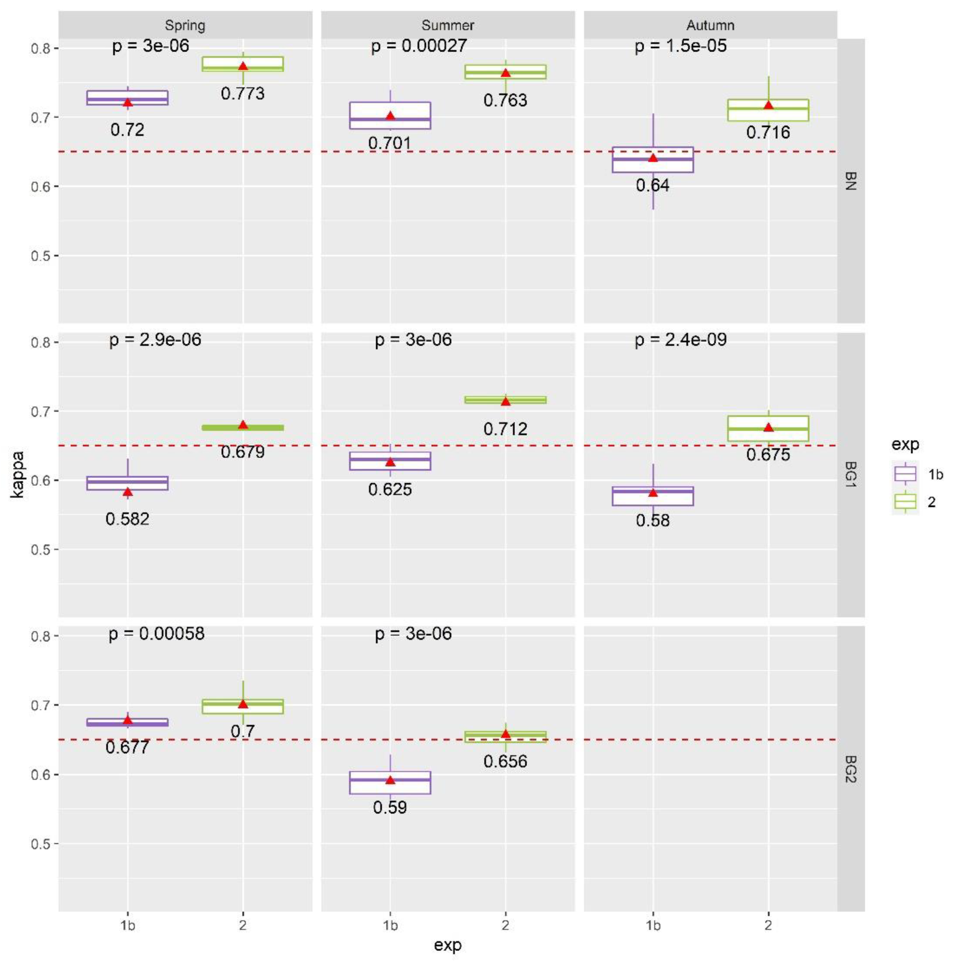
3.5.2. Exp. 2: LiDAR Products and Spectral Indices

After the dimensionality reduction technique had been selected, the following objective was to investigate which other input features could increase the classification accuracy achieved in Exp. 1a/1b by using the HS dataset alone. For this purpose, the 93 LiDAR indices and the 65 SI computed in Section 3.2 were all added as input features in the Exp. 2 (see also Figure 5). The same ten manually generated training/validation shapefiles used in Exp. 1a/1b were also adopted for this experiment (Table 2). The RFE technique (Section 3.4) was also employed during RF classification, using the same approach as described in Exp. 1a.

The aim this time was to analyze the lists of optimal feature selections among the ten different runs and then finding a certain number of commonly selected features which might represent the best-to-use HS and ALS features to map the selected meadows and dry grasslands habitats.

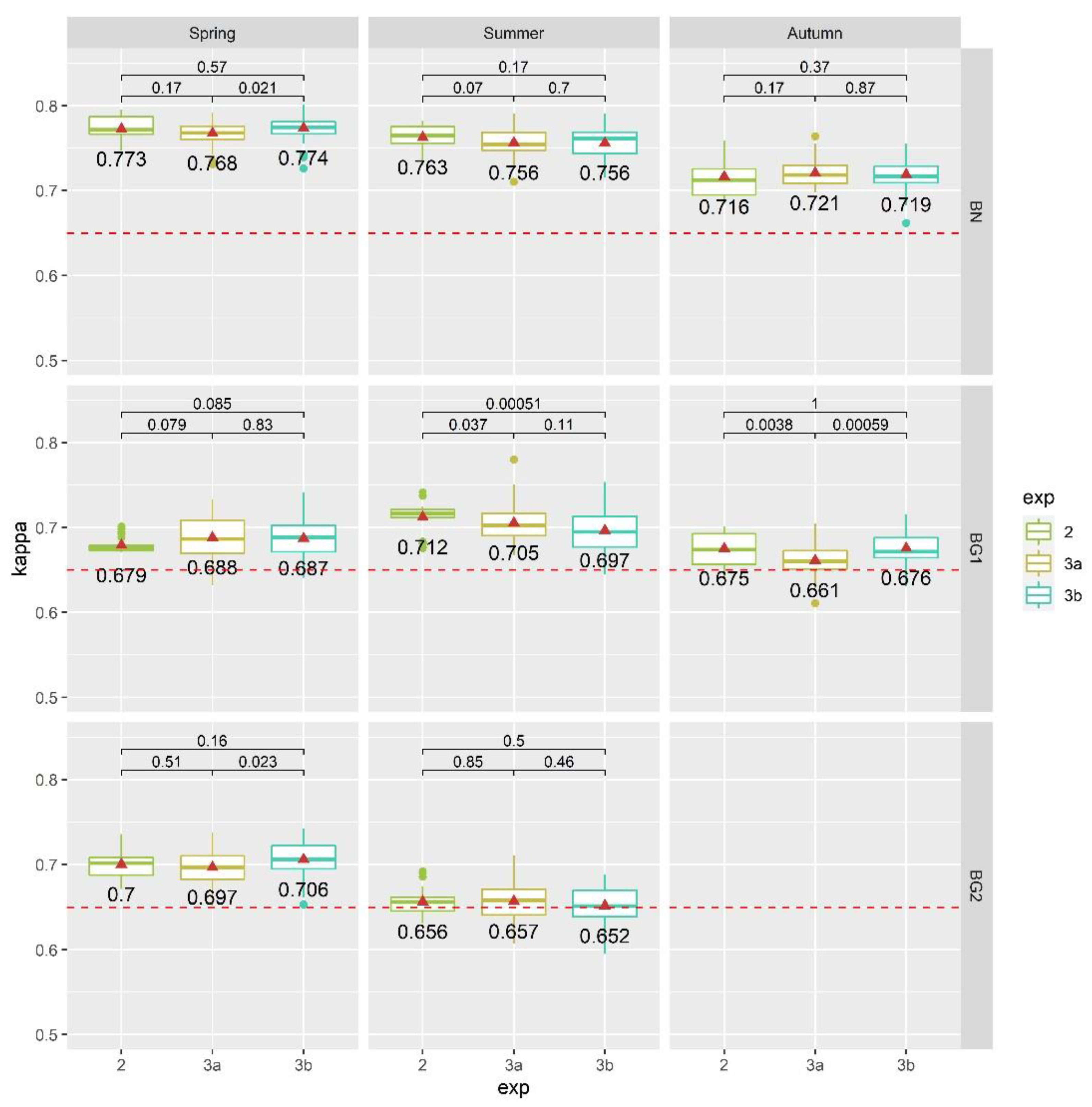
3.5.3. Exp. 3: Feature Selection Validation Attempt

The objective of this last experiment was two-fold: verifying that the optimal features were properly selected in Exp. 2 and attempting a generalization of the selected optimal features among the different study areas analyzed. The RF classification was therefore run using only the selection of best-to-use features resulting from Exp. 2, not on the entire list of features generated by HS and ALS pre-processing (Figure 5). Obviously, in this case the RFE technique was not used during RF classification (Table 2). Moreover, the splitting between training/validation polygons was done automatically by the software on a 50/50 random basis and repeated for 50 different runs, so to have 50 different RF classification results (Table 2). In this way, a much higher statistical distribution of Kappa results, based on the optimal features selection, can be investigated and discussed as compared to Exp. 2.

In order to decide which optimal feature selection would be better, single features were used in Exp. 3 if selected at least 50% of times, based on two different approaches:

• Exp. 3a: the selection of optimal features was done separately for each area, meaning that a different best-to-use features selection was used for each case study, as a result of Exp. 2;
• Exp. 3b: the selection of optimal features was the same for all study areas, meaning that a unique best-to-use features selection was extrapolated from all study areas at the same time, as a result of Exp. 2.

By performing these two separate experiments we can test: (1) How the RF classification performs when using a very limited number of features; (2) how a different selection of best-to-use features could affect the classification results; and (3) attempt to generalize a best-to-use features selection for the classification of the investigated habitats over the three selected study areas.

4. Results

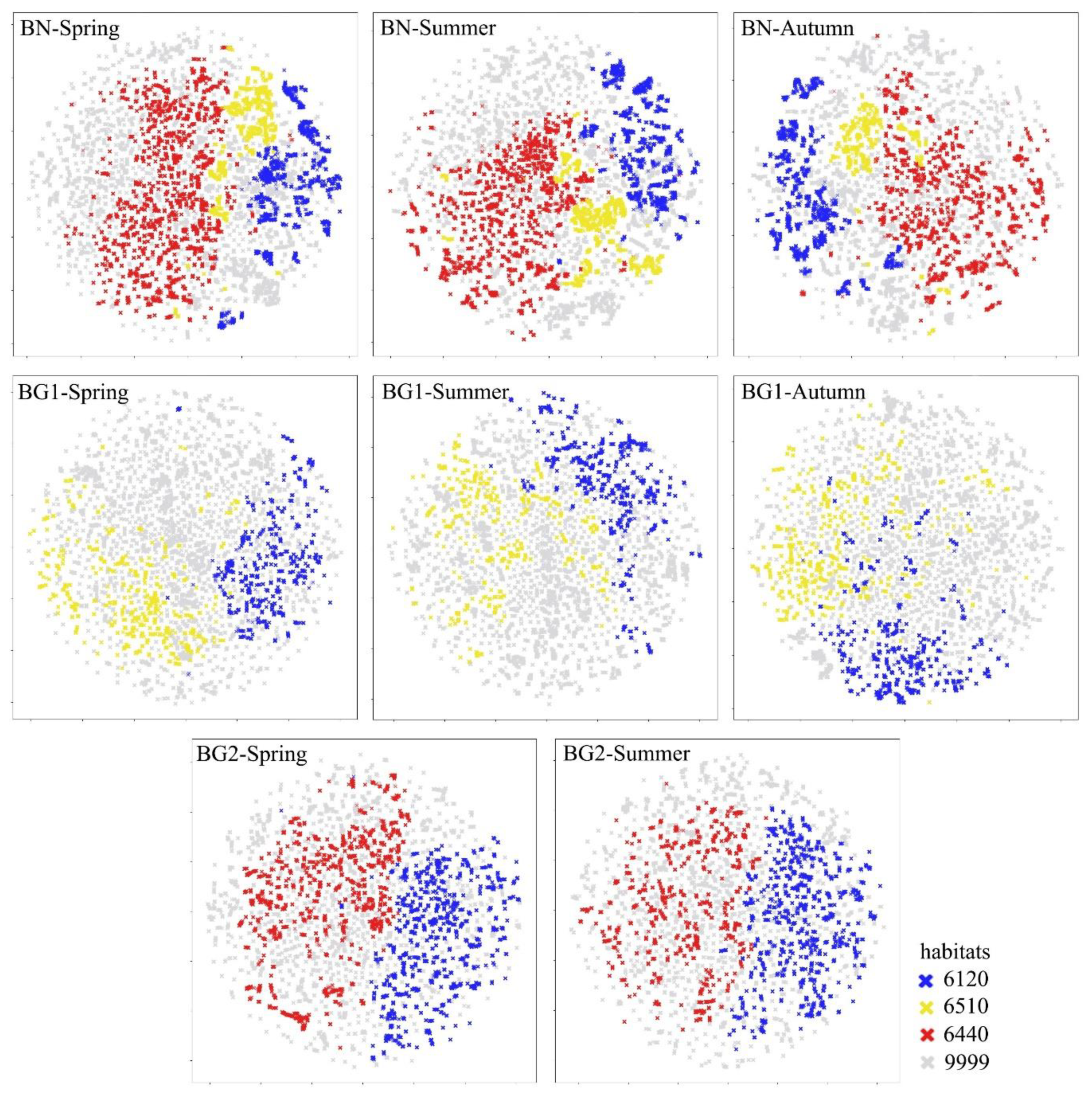
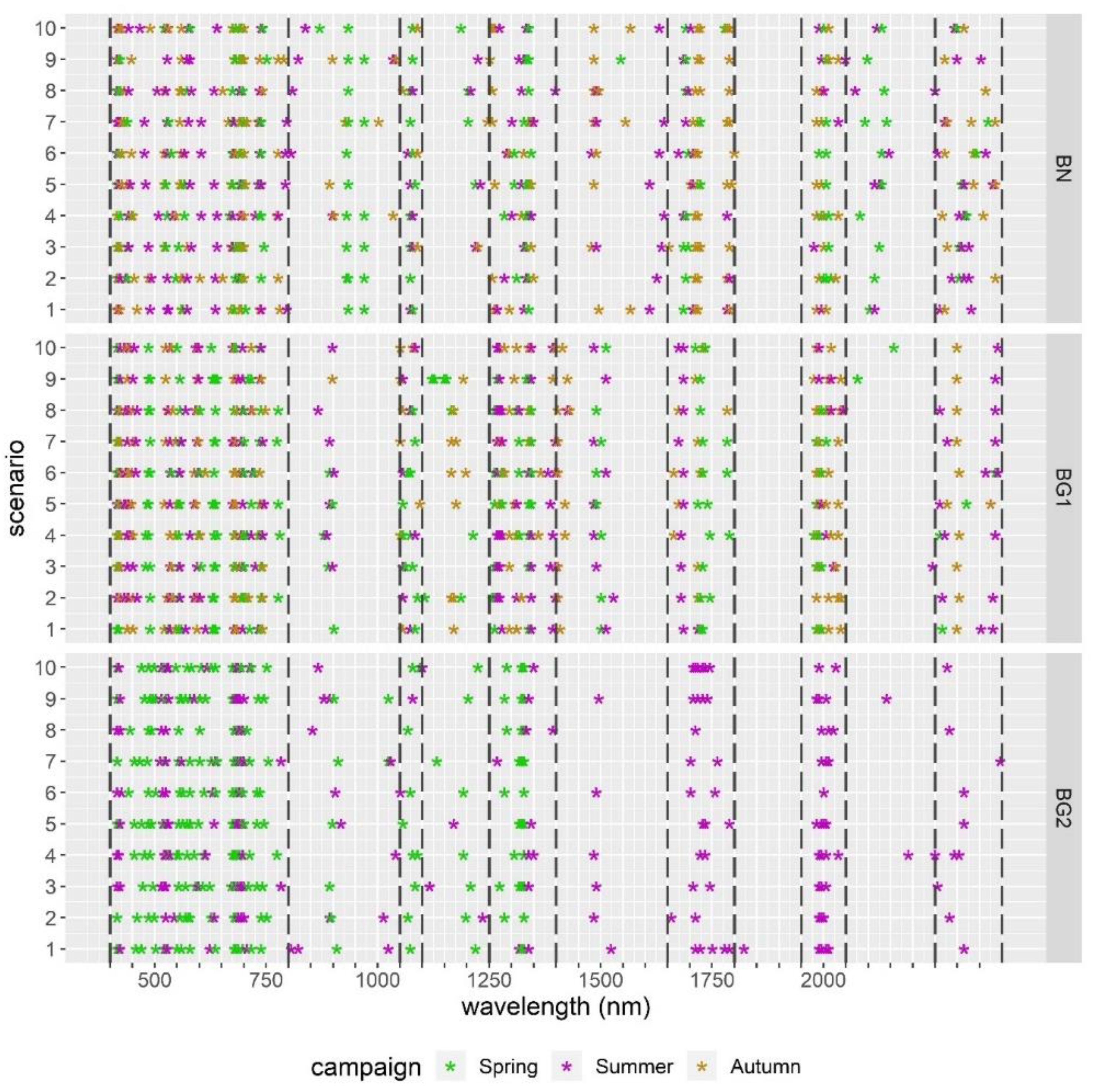
4.1. Results of Exp. 1

The best-to-use spectral channels selected by the RFE technique (based on the approach described in Section 3.4) when classifying the 430 SR bands (Exp. 1a) are plotted in Figure 7, for each study area and for each acquisition campaign (different colors). The results show that the mostly used spectral channels belong to the following spectral ranges:

• 400–800 nm of the visible spectral range (mainly red and blue);
• 1050–1100 nm of the near-infrared;
• 1250–1400 nm, 1650–1800 nm, 1950–2050 nm, and 2250–2400 nm of the SWIR spectral range.

For each of the ten RF classification runs (scenario 1-10, as explained in Table 2), the Kappa accuracies obtained by the optimal features selection after applying the RFE (Exp. 1a) are plotted in Figure 8 against the Kappa accuracies obtained by classifying the 30 MNF components alone (Exp. 1b). The ƿ-value resulting from the “Wilcoxon signed-rank test” [95] are also plotted. A ƿ-value less than 0.01 (typically ≤ 0.01) indicates that there is a statistically significant difference between the two results, while on the contrary for a ƿ-value higher than 0.01, there is not a statistically significant difference [96]. If we compare all results, we can observe that in all cases the MNF results outperform the RFE results, with statistically significant difference. For example, for the BN spring acquisition, the MNF results (Exp. 1b) have a mean Kappa of 0.72, while the RFE results (Exp. 1a) have a mean Kappa of 0.656. As another example, for the BG2 summer acquisition, the MNF results have a Kappa of 0.59, while the RFE results have a Kappa of 0.521. For this reason, the 30 MNF components were retained for further processing and Exp. 2 was run by adding all others input features (93 LiDAR-products and 65 SI) to the 30 MNF components, as described in Section 3.5.2 and Figure 4.

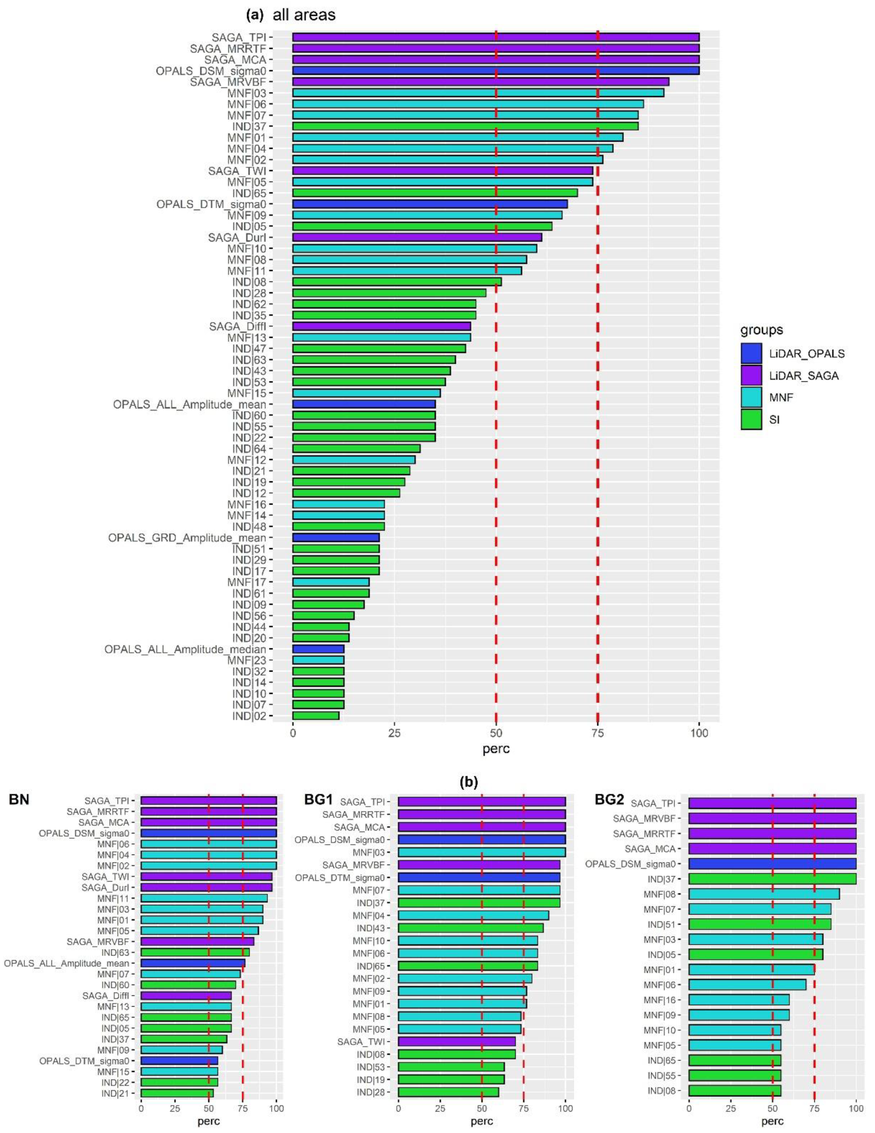
4.2. Results of Exp. 2

The Kappa accuracies of Exp. 2 are summarized and compared to the Kappa accuracies of the Exp. 1b in Figure 9. The ƿ-values resulting from the “Wilcoxon signed-rank test” are also plotted. As we can see, the accuracy is increased when adding LiDAR and SI features (Exp. 2) in a statistically significant way for all cases analyzed: the ƿ-values are always lower than the significance level of 0.01. Moreover, the final classification accuracy is now higher than a tolerance level of K = 0.65 (red dotted line in Figure 9) for all Exp. 2 results. For each run of the ten runs in Exp. 2, an optimal selection of features was extracted (as explained in Figure 6, Section 3.4) and a frequency distribution of most selected features was computed. This can be done either considering all the study areas together, or area by area, as illustrated in Figure 10.

The results show that there are features being selected 100% of times for all study areas (Figure 10a) by the RFE-RF, in particular:

• SAGA_TPI (topographic position index);
• SAGA_MRRTF (multiresolution index of the ridge top flatness);
• SAGA_MCA (modified catchment area);
• OPALS_DSM_Sigma0: DSM standard deviation of the unit weight.

Other features are selected more than 75% of times by the RFE-RF, in particular:

• SAGA_ MRVBF (multiresolution index of valley bottom flatness);
• SAGA_TWI (topographic wetness index);
• Spectral MNF components [1:7];
• Spectral Index nr.37 (NDNI: normalized difference nitrogen index).

The area-related frequency distributions (Figure 10b) reveal some variability in the mostly used features. For example, for the BN study area, also the MNF components [02,04,06] were selected for all scenarios (100% of times). Other features selected more than 75% of times are:

• LiDAR products: SAGA_TWI, SAGA Duration of Insolation (SAGA_DurI), OPALS mean amplitude (ALL_Amplitude_mean), SAGA_MRVBF;
• SI: nr.63 (WV-NHFD: WorldView non-homogeneous feature difference);
• Spectral MNF components: [01,03,05,07,11].

For the BG1 area, also the MNF component 03 was selected 100% of times. The other features selected more than 75% of times are:

• LiDAR products: SAGA_ MRVBF and OPALS_DTM_sigma0 (DTM standard deviation of the unit weight);
• SI: nr.37 (NDNI), nr.43 (PRI: photochemical reflectance index), nr.65 (WVWI: WorldView Water Index);
• MNF components: [01;02;04-10].

For the BG2 area, also the SAGA_ MRVBF and SI nr.37 (NDNI) were selected 100% of times. The other features selected more than 75% of times are:

• SI: nr.51 (SIPI: structure insensitive pigment index) and nr.05 (CRI1: carotenoid reflectance index 1);
• MNF components: [01;03;07,08].

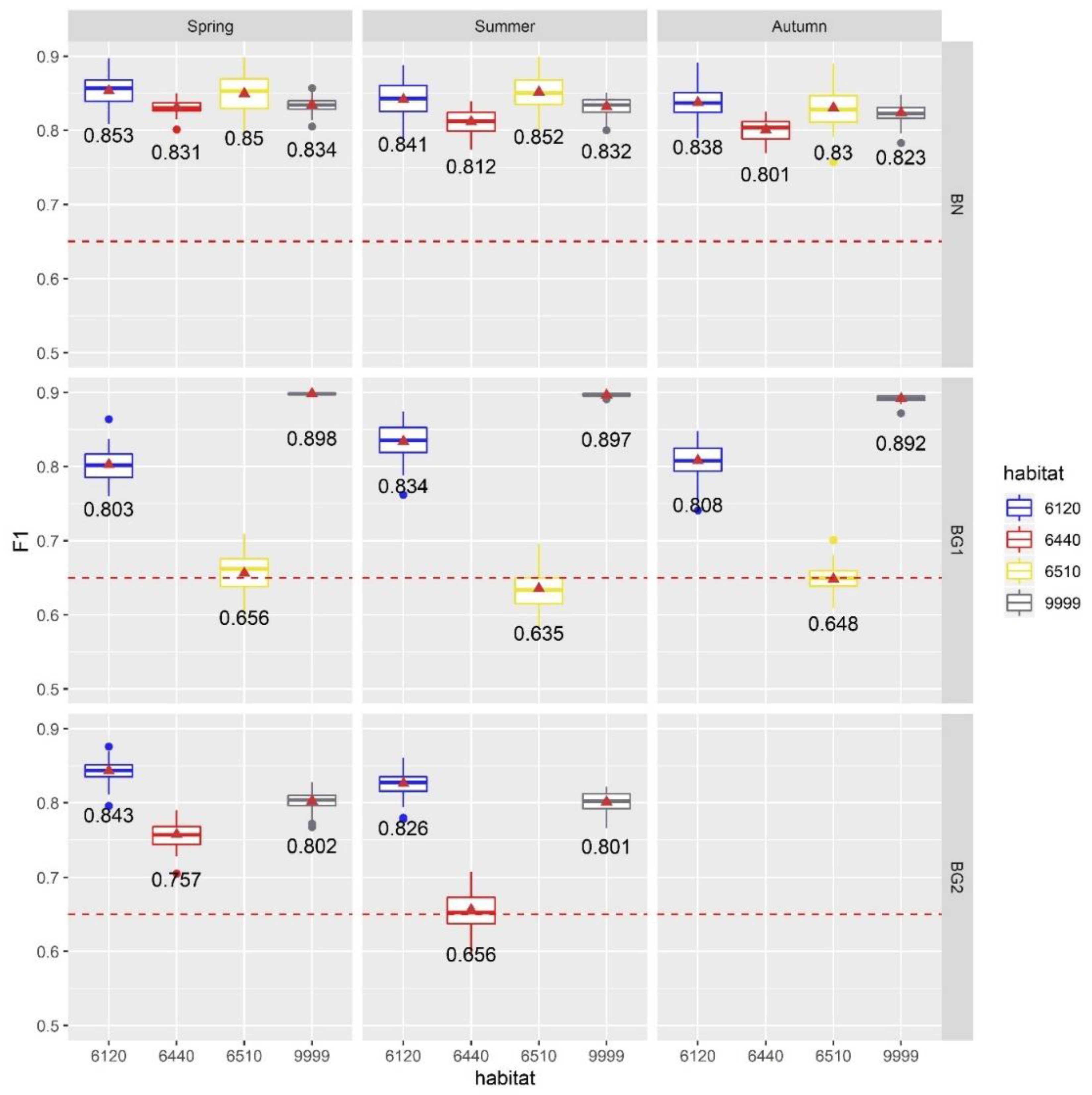
4.3. Results of Exp. 3

The results of Figure 10 were used as a supportive tool to decide which features are to be used for the next Exp. 3a (area-by-are feature selection) and Exp. 3b (selection based on all study areas together). Therefore, a list of features was produced and is presented in

Table 3. List of features selected more than 50% of times from Exp. 2 and used in Exp. 3a/3b, with corresponding explanations and references. Colors in the right columns mean that the feature was used in the corresponding experiment (3a or 3b). The different colors are associated to different feature groups, using same coloring as in Figure 10.

				Exp. 3a			Exp. 3b
				BN	BG1	BG2	ALL
LiDAR OPALS:	Category:	Input Layers:	Ref.:
ALL_Amplitude_mean	Morphology	DTM	-
DSM_sigma0	Morphology	DSM	-
DTM_sigma0	Morphology	DTM	-
LiDAR SAGA:
DiffI (Diffuse Insolation)	Light availability	DSM	[97,98]
DurI (Duration of Insolation)	Light availability	DSM	[97,98]
MRRTF (Multiresolution Index of the Ridge Top Flatness)	Morphology	DTM	[99]
MRVBF (Multiresolution Index of Valley Bottom Flatness)	Morphology	DTM	[99]
TPI (Topographic Position Index)	Morphology	DTM	[98,100]
MCA (Modified Catchment Area)	Wetness	DTM	[101]
TWI (Topographic Wetness Index)	Wetness	DTM	[101]
Spectral Indices:
5-CRI1: Carotenoid Reflectance Index 1	Leaf Pigments	510, 550	[102]
7-CAI: Cellulose Absorption Index	Dry or Senescent Carbon	2000, 2200, 2100	[103]
8-CM: Clay Minerals Ratio	Geology Indices	1550–1750, 2080–2350	[104]
12-GEMI: Global Environmental Monitoring Index	Broadband Greenness	650, 850	[105]
19-IO: Iron Oxide Ratio	Geology Indices	450–520, 630–690	[104,106]
21-MCARI: Modified Chlorophyll Absorption Ratio Index	Narrowband Greenness	550, 670, 700	[107]
22-MCARI2: Modified Chlorophyll Absorption Ratio Index Improved	Narrowband Greenness	550, 670, 800	[108]
28-MTVI: Modified Triangular Vegetation Index	Narrowband Greenness	550, 670, 800	[108]
35-NDLI: Normalized Difference Lignin Index	Dry or Senescent Carbon	1680, 1754	[109,110]
37-NDNI: Normalized Difference Nitrogen Index	Canopy Nitrogen	1510, 1680	[109,110]
43-PRI: Photochemical Reflectance Index	Light Use Efficiency	531, 570	[111,112]
51-SIPI: Structure Insensitive Pigment Index	Light Use Efficiency	445, 680, 800	[113]
53-TCARI: Transformed Chlorophyll Absorption Reflectance Index	Narrowband Greenness	550, 670, 700	[108]
55-TVI: Triangular Vegetation Index	Narrowband Greenness	550, 670, 750	[114]
60-WV-BI: WorldView Built-Up Index	Other	450, 730	[115]
62-WV-II: WorldView New Iron Index	Geology Indices	550, 600, 470	[115]
63-WVNHFD: WorldView Non-Homogeneous Feature Difference	Other	450, 730	[115]
65-WV-WI: WorldView Water Index	Other	450, 870–1040	[115]
MNF components:
MNF 1, 3, 5, 6, 7, 9	-	-	-
MNF 2, 4	-	-	-
MNF 8, 10	-	-	-
MNF 11	-	-	-
MNF 13, 15	-	-	-
MNF 16	-	-	-
Total number of used features				28	26	24	24

, with corresponding explanation of each indicator. For Exp. 3b a fixed number of 24 features are to be used, while for Exp. 3a between 24 and 28 features are to be used, depending on the study area. The main difference consists in the different SI being selected from one study area to another. In fact, only the NDNI and WVWI indices were always selected for the three study areas. Similarly, from the LiDAR products, MRRTF, MRVBF, TPI, MCA, DSM_Sigma0 are all being used for all study areas. From the MNF components, only some of them were used for all study areas, strengthening the spectral heterogeneity of the different habitats’ classes within the study areas analyzed.

In Figure 11, the Kappa values of Exp. 3a/3b for all areas and acquisitions are plotted and compared with respect to Exp. 2. The ƿ-values resulting from this comparison are also plotted. The Kappa values are very similar for most classification results and in most study areas analyzed. Apart from some exceptions in BG1 area, the ƿ-values are mostly higher than the significance level of 0.01, meaning that in general terms there are no significant differences between Exp. 2, 3a, or 3b. For the summer acquisition of the BG1 area, Exp. 2 and Exp. 3a have no significant difference, while Exp. 3b resulted in a statistically significant lower accuracy (K = 0.697 instead of K = 0.712). The opposite occurs for the autumn acquisition of the BG1 area, where Exp. 2 and Exp. 3b have no significant difference, while Exp. 3a produced a significantly lower accuracy (K = 0.661 instead of K = 0.675). On the other hand, for the spring acquisition of BG1 area, Exp. 3a and Exp. 3b generated a slightly higher mean Kappa, with a statistically significant difference in respect to Exp. 2. This is the only case in which Exp. 3 significantly outperformed Exp. 2. For the BN study area, the highest Kappa are obtained in the spring and summer acquisitions, with mean values ranging from 0.768–0.774 and 0.756–0.763, while in the autumn acquisition the values are in the range 0.716–0.721. Lowest values for the autumn acquisition are also noticed for the BG1 study area, in the range 0.661–0.675, whereas spring and summer values are in the ranges 0.679–0.688 and 0.697–0.712 respectively. For the BG2 study area, the highest values are recorded for the spring acquisition, in the range 0.697–0.706, while for the summer acquisition the mean Kappa values are in the range 0.652–0.657.

Considering that only in one case (BG1-Summer) the Exp. 3b produced significantly lower accuracies, while in all other cases no significantly reduction in classification was remarked, the final classification maps were produced with the Exp. 3b selected features (Table 3) and are plotted in Figure 12.

Figure 13 displays also the resulting F1 accuracies of these RFE-RF results, computed for each habitat and area. For the BN area, F1 values are pretty high and uniform for all the three analyzed habitat classes. The mean F1 values for the habitat 6120 are in the range 0.838–0.853. Similar values are obtained for habitat 6510, with values in range 0.830–0.852. The background class 9999 scores a bit lower with values in range 0.823–0.834. Finally, the lowest scoring class is habitat 6440, with values in the range 0.801–0.831. For BG1 area, the background class and habitat 6120 have rather high F1 accuracies for both acquisitions: 0.892–0.898 and 0.803–0.834 respectively. Whereas, the habitat 6510 produced rather low accuracies in all acquisitions ranging only between 0.635 and 0.656. In the BG2 area habitat 6120 has a similarly high level of F1 accuracies as compared to other study areas BN and BG1. Mean values in fact range between 0.826 and 0.843. Similarly, it happens for the 9999 class with values around 0.801–0.802. On the other hand, habitat 6440 produced lower F1 as compared to BN study area: for the spring acquisition the mean value is 0.757, while for the summer acquisition it is only 0.656.

5. Discussion

5.1. The Importance of Different Hyperspectral Channels and Dimensionality Reduction Techniques for Mapping Meadows and Dry Grasslands Habitats in the Selected River Valleys

The Exp. 1 was designed with the aim of identifying the most relevant hyperspectral channels, required to classify the selected meadows and dry grasslands habitats (code 6440, 650, and 6120) and to choose the most efficient dimensionality reduction technique between RFE and MNF.

Because the spectral heterogeneity of each habitat class was pretty high due to strong variability in habitats’ species composition, we decided to realize ten different training/validation selections and therefore run ten different RF classifications. In this way, results can be considered more reliable and less influenced by an individual sample selection. When applying the RFE technique on the 430 SR bands, a similar pattern of spectral bands was selected among the ten different classification scenarios realized for each study area and acquisition period. The obtained results emphasized the importance of HS information for mapping the investigated habitats, especially of the SWIR channel. Both habitats are in fact characterized by very different soil moisture conditions, therefore it is probable that the spectral information contained in the SWIR channel is a key source of information to enable distinguishing such types of grasslands habitats.

When comparing the Kappa accuracies, we found that MNF transformation is a better and more effective technique for removing the inherent noise in the hyperspectral data cube without losing the relevant spectral information required to obtain a higher level of classification accuracy. On the other hand, the RFE technique, although reducing the number of spectral bands during classification, loses part of the inherent spectral information in a way that the classification performances are reduced in a statistically significant manner: Kappa values were rather low and around 0.50-0.55 in most cases analyzed. The major drawback of MNF transformation is that the transformed bands have no physical meaning and cannot provide insights on the spectral channels of importance for the classification of the selected habitats.

Despite of the fact that RFE is not able to maintain classification accuracies as high as MNF method, the results of Exp. 1 have proved its usefulness as a tool to highlight and identify which hyperspectral channels are mostly used for the investigated habitats classification. Something that is not possible to perceive with the MNF technique alone. This is an important information to shed lights on the spectral configuration requirements for monitoring these Natura 2000 habitats, for example in view of future hyperspectral data acquisition mission planning. Nevertheless, the rather low levels of Kappa accuracies obtained even when using the MNF components alone (mostly K<0.65), suggest the need of other sources of data in order to get a higher and more satisfiable level of classification accuracy for mapping the selected habitats.

5.2. LiDAR Products and Spectral Indices Selection to Enhance Habitats Classification Performances

The Exp. 2 was designed with the aim of understanding which LiDAR and SI products are to be produced for the investigated classification problem and if these extra input features might enhance the rather low classification accuracies obtained by using the HS dataset alone (mostly with K < 0.65, Exp. 1b). In line with other studies focusing on mapping similar habitat types [50], the integration of LiDAR-derived products and SI obtained from different spectral bands has proven to be a good solution for getting higher classification accuracy. In fact, in most study areas, the Kappa values have scored a statistically significant increase, reaching a quite satisfiable result (K > 0.65). This is a great achievement, considering the very challenging task of being able to automatically distinguish different types of selected Natura 2000 habitats, characterized by a high within-class heterogeneity. These natural grasslands are in fact composed by a high variability of species, described by different spectral characteristics within the same habitat class. At the same time, they can be very similar to each other and present similar spectral characteristics with respect to other non-habitats vegetation patches (background class 9999) that are found in the studied river valleys. The combination of all these aspects, makes their automatic identification in a natural landscape a very challenging task.

5.2.1. LiDAR-Based Features of Importance

The frequency distributions of the selected features of importance revealed the great influence of the LiDAR-based products, especially computed from the SAGA software. In fact, the three morphological indicators (TPI, MRRTF, and MCA) proved to be fundamental inputs to reach a good classification level, because they are selected 100% of times. Among them, the multiresolution index of the ridge top flatness (MRRTF) is a topographic index designed to identify high-flat areas at different scales. It complements the multiresolution index of valley bottom flatness (MRVBF) that instead is designed to identify areas of deposited material in flat valley bottoms [99].

The dependence of habitats types occurrence to different topographical characteristics of the landscape, justifies the selection of these indicators as the most important selected features. In fact, the lowland hay meadows (habitat 6510) found in Biebrza and Bug river valleys, are characterized by plant communities which often arise outside the floodplain, in higher terraces where floods or inundation do not occur [80], therefore with probably higher MRRTF values. On the other hand, alluvial meadows (habitat 6440) are usually found in shallow depressions of the floodplain [5], that might be depicted by low MRVBF values. Finally, dry grasslands (habitat 6120), are associated with sandy deposits, forming extensive flat elevations both on the floodplain and on higher terrace levels, described by spatially different values of MRRTF and MRVBF. Similarly, the topographic position index (TPI), has been reported to be useful to classify the landscape into slope position (i.e., ridge top, valley bottom, etc.,) and landform category (i.e., gentle valleys, plains, open slopes, etc.) [100]; moreover, also species distribution models showed significant relationships to TPI in [116].

The modified catchment area (MCA), together with the topographic wetness index (TWI), have been developed for predicting the spatial distribution of soil moisture contents in hilly terrains [101] and have been reported to be important indicators for describing floods [117], which are a very recurrent and important phenomenon in the Biebrza and Bug river valleys investigated in this work (Section 2.1). In fact, habitats 6510, 6440, and 6120 are all strictly connected to periodic floods. Plant communities of lowland hay meadows (habitat 6510) and dry grasslands (habitat 6120) are beyond the reach of the flood and inundations [80,81], while alluvial meadows (habitat 6440) communities are able to adapt to changing moisture contents and are found in shallow depressions of the floodplain, characterized by temporary flooding [5].

It is remarkable seeing that the most important features being selected by the RFE-RF system are exactly those topographic and wetness indicators (TPI, MRRTF, MRVBF, MCA, and TWI) that better portray the characteristics of the Natura 2000 habitats found in our investigated study areas, along both the Biebrza and Bug river valleys.

5.2.2. Spectral Indices of Importance

The spectral indices (SI) computed under the ENVI software, using different HS channels, have also proven to be among the most important features to be used for classification. However, their importance and impact are less evident than the topographic-based features described above. Figure 10 clearly showed that the selection of each index is more scattered and linked to specific areas and therefore probably to local habitats conditions. In fact, by their nature, SI are meant to picture very specific vegetation conditions, that might be difficult to generalize for large and highly heterogenous plant communities, as they might be more suited to describe local-specific phenomena or only some specific habitats. Different categories of indices were selected by RFE-RF during Exp. 2 (Table 3). In this section we will discuss the most relevant and common ones.

The canopy nitrogen indices measure the nitrogen concentration in vegetation, which is an important component of chlorophyll and which is present in high concentrations in quickly growing vegetation. Among this group, the normalized difference nitrogen index (NDNI) was designed with the aim of measuring the relative estimate of nitrogen in vegetation canopies, the sensitiveness of leaves to nitrogen concentration as well as the overall foliage biomass of the canopy [109]. It is based on the 1510 nm and 1680 nm spectral bands, both in the SWIR part of the electromagnetic spectrum. The NDNI is one of the most important SI, used more than 75% times to classify our habitats among all study areas analyzed. This result is in line with the results obtained when analyzing the mostly used spectral channels of the HS dataset (Section 5.1) and highlights the importance of having the SWIR part of the electromagnetic spectrum measured.

Leaf pigments indices measure the stress-related pigments, which are present in higher concentrations in weakened vegetation. Among this group, the carotenoid reflectance index 1 (CRI1) is a measure of stressed vegetation, based on the level of carotenoid concentration, which regulate the light absorption processes in plants [102]. The CRI1, computed with 510 nm and 550 nm spectral bands, is another important feature selected by the RFE-RF system most of the times for the investigated study areas. Another important selected SI is the clay mineral ratio (CM), a band ratio working in two different regions of the SWIR spectral range, aimed at highlighting the presence of clay. Lowland hay meadows (habitat 6510) have been reported to originate in mineral soils, with high share of silt or clays [5,79], while dry grasslands (habitat 6120) have been reported to develop on sandy soils [81]. The dependence of habitats types occurrence to different soil types justifies the selection of CRI1 as an important selected feature. Moreover, the WorldView water index (WVWI), designed to highlight areas of standing water [115] and working in the NIR and blue spectral ranges, is also selected among the most important features for the selected study areas, reflecting the different moisture content of the investigated habitats [5].

A number of Narrowband Greenness indices is also selected in the different acquisitions and study areas analyzed (Table 3). They are a combination of reflectance measurements in the green, red and NIR spectral ranges aimed at measuring the overall amount and quality of photosynthetic material in vegetation, which is essential for understanding the state of vegetation [107,108]. Among these, three types of indices dedicated to the estimation of chlorophyll abundance are selected (MCARI, MCARI2, TCARI) and two types dedicated to the estimation of green leaf-area-index (TVI and MTVI).

The light use efficiency indices are highly linked to the carbon uptake, somewhat related to fractional absorption of photosynthetically active radiation (fAPAR). Among this group, the photochemical reflectance index (PRI), mainly selected for BG1 area, is used in studies of vegetation health and agricultural crops productivity and stress [111,112]. Besides, the structure insensitive pigment index (SIPI), developed to assess canopy stress [113], is selected several times for BG2 area.

The dry or senescent carbon indices provide an estimate of the amount of carbon in dry states of lignin and cellulose. Among this group, the cellulose absorption index (CAI) highlights dried plant materials, because of absorptions in the 2000–2200 nm range to cellulose [103]. Similarly, the normalized difference lignin index (NDLI), using 1680 nm and 1754 nm spectral bands, provides an estimation of the relative amounts of lignin contained in vegetation canopies [109]. Both NDLI and CAI are selected only for BG2 study area. This index might operate as an indicator of dryness, a characteristic of habitats 6120 [81]; this might explain why it was selected. Finally, two geology indices, iron oxide ratio (IO), and WorldView new iron index (WVII) are selected for BG1 and BG2 areas respectively.

The scattered selection of different spectral indices has well pictured the spectral heterogeneity nature of the investigated habitats. In fact, habitats 6120, 6440, and 6510 are both characterized by a high variability in terms of species composition as well as physiognomy [75,76], which both contributes to the selection of different SI depending on the area and habitats analyzed. However, among the selected SI, the most important ones are computed using the SWIR channels and subsequently the NIR and visible parts of the spectrum.

5.2.3. Best-to-Use HS+ALS Products for Mapping Meadows and Dry Grasslands Habitats in the Selected River Valleys

The last set of experiments (Exp. 3a and Exp. 3b) was designed with the aim of verifying the appropriateness of the optimal features selection. In the first case (Exp. 3a), the optimal features were selected area by area, while in the latter case (Exp. 3b) a common feature selection was performed considering the three study areas together. From this feature selection exercise, it was revealed that spectral indices are more dependent on the individual study areas (different SI selected for different study areas), while the LiDAR products are more uniform over the three study areas. This could be explained by the fact that the topographical microrelief variability is more homogeneous among the analyzed river valleys, while SI, depicting different vegetation characteristics and conditions (e.g.,: vegetation stress, chlorophyll/nitrogen concentrations, moisture content, etc..), have by nature a higher local spatial variability.

The classification results showed very similar outcomes in most cases analyzed (both Exp. 3a and 3b), demonstrating the effectiveness of the RFE-RF system for classification and feature selection. With a much lower number of features, 24-28 instead of 188, it was possible to reach similar performances in terms of classification accuracies, at the same time reducing processing time and data handling. Moreover, reliability of results was also increased by using 50 classification runs, based on random training/validation selections, instead of only 10.

Because of the fact that almost no significant reduction of classification accuracy was recorded when generalizing the feature selection to the three areas (Exp. 3b), the final classification results were produced using the 24 features identified by this common feature selection, in particular (Table 3):

• LiDAR (SAGA) products: DurI, MRRTF, MRVBF, TPI, MCA, TWI;
• LiDAR (OPALS) products: DSM_Sigma0, DTM_Sigma0;
• SI: CR1, CM, NDNI, WVWI;
• MNF: 1-11.

Therefore, we can claim that the optimal feature selection generalization attempt was a reliable choice. Similar classification accuracies can be produced when using the same selected features for the three study areas, without the need to calculate several other products area by area. By generalizing the feature selection, however, several other area-dependent SI are not used for classification (Table 3). This might cause, in some exceptional cases, slight reductions in Kappa values, as reported for example in BG1-summer acquisition (from K = 0.712 to K = 0.697).

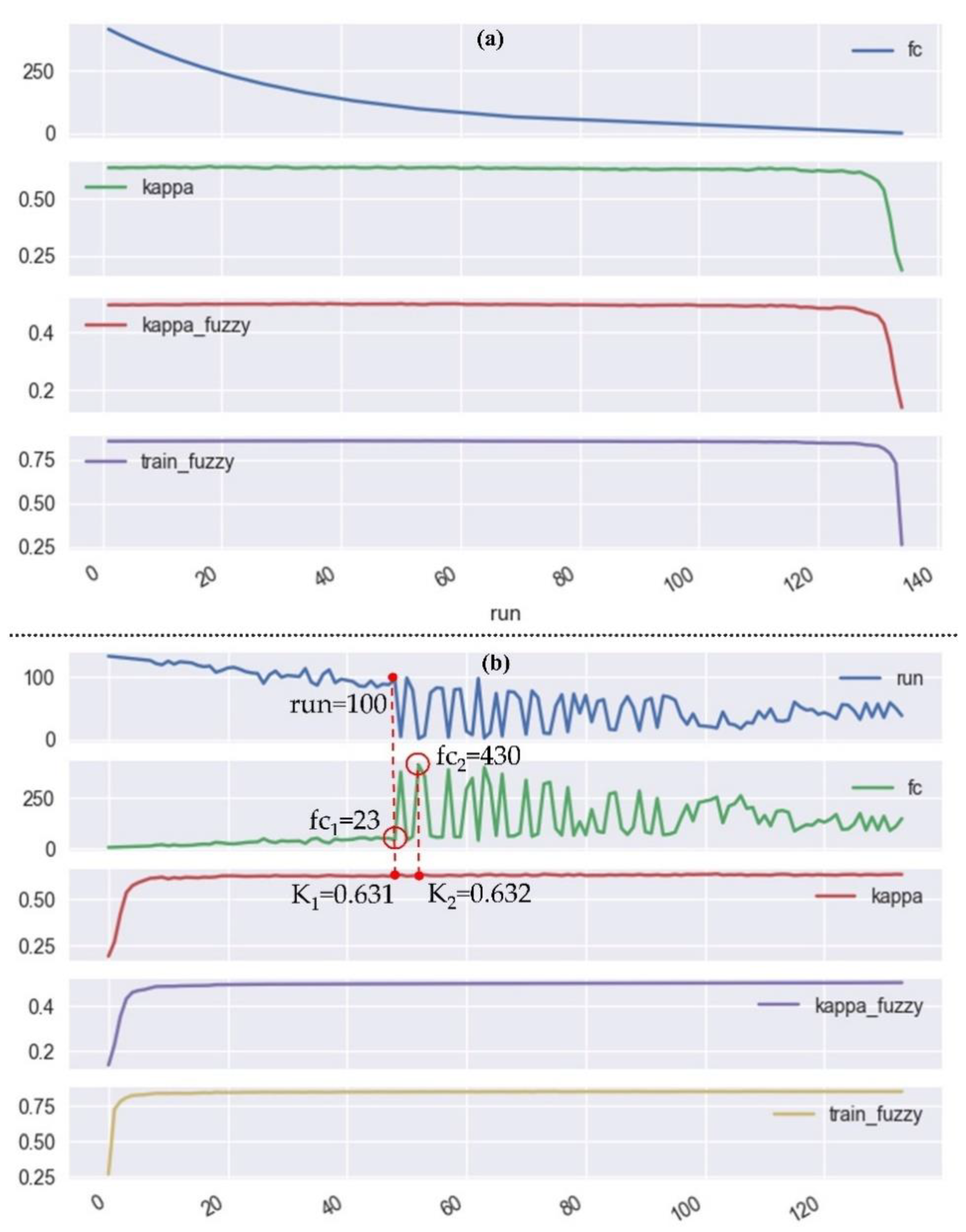
5.3. Considerations on the Computational Efficiency of the RFE-RF System

The RF-RFE system proved to be beneficial from the computational performance point of view. The only upfront cost is that over hundred models had to be learned in sequence to obtain the optimized set of features. However, this needs to be done only once per dataset, then the successive prediction phase can benefit from it. The prediction phase is the most demanding one, because it is applied on the entire pixels (and features) in the whole study areas. Therefore, every eliminated feature results in faster prediction time, since less data have to be read from disk, transferred over the network, and processed by the CPU. Typically, by using only 1/3 of the original number of features, we can expect roughly even 3x decrease of our prediction time. In our case, classification times were in the range of minutes for training and below half an hour for predicting the whole study area (on a modern, budget machine), so performance considerations were not very critical. But especially for larger and more complex datasets we consider implementing the RF-RFE procedure a win-win situation, providing considerable savings in computational effort without losing in terms of final classification accuracy.

6. Conclusions

The main objective of this study was to develop an automated system based on recursive feature elimination and random forest classification (RFE-RF), capable of complementing the potentiality of RF classification and RFE feature selection, for the mapping of selected Natura 2000 meadows and dry grasslands (habitats 6120, 6440, and 6510) along Polish river valleys by the fusion of airborne Hyperspectral and LiDAR data. For this purpose, multiple flight acquisitions were performed along Biebrza and Bug river valleys (Poland) and extensive field-botanical activities were conducted to built-up a reliable database to be used as a reference for the classification. Several experiments were performed to test the different potentialities of the RFE-RF system and to tackle several research questions. The conclusions we can draw from the results of this work are as follows:

• The MNF dimensionality reduction method outperformed RFE: part of the inherent spectral information was lost during RFE feature selection and therefore the classification accuracy significantly reduced. On the other hand, with the RFE technique, it was possible to highlight the important HS channels that are necessary for mapping the investigated habitats: VIS, NIR, and SWIR are all required spectral channels;
• By selecting and using only the original input bands, without any kind of data-transformation, the RFE-RF system proved to be a very efficient and useful setup for automated hyperspectral and LiDAR data processing, highlighting the added value of the fusion between these complementary and diverse datasets. It is therefore possible to use a common selection of 24 features (instead of 188) to distinguish the investigated habitats of this study and still obtain very similar classification accuracies among all considered study areas;
• LiDAR-based products, depicting the variable topographic micro-reliefs of the investigated river valleys, proved to be the most selected features producing also a significant enhancement in the classification accuracy. In particular: topographic position index (TPI), multiresolution index of the ridge top flatness (MRRTF), multiresolution index of valley bottom flatness (MRVBF), modified catchment area (MCA), topographic wetness index (TWI), DSM_Sigma0 and DTM_Signma0 proved to be necessary adjuncts for mapping Natura 2000 habitats 6120, 6440 and 6510;
• The meaningfulness of the selected products is strongly linked to the habitats’ characteristics. It was remarkable noticing that since habitat 6510 is mostly found in higher terraces, while habitat 6440 is usually found in low depressions of the floodplain, the MRRTF and MRVBF products were retained as the most relevant classification features. In fact, MRRTF and MRVBF have been conceived for the identification of high-flat areas and flat valley bottoms respectively [99]. Likewise, since habitats 6120, 6510, and 6440 are all connected to periodic floods in different ways, the TWI and MCA products, reported in literature to be good indicators of floods [101], have also been selected as best-to-use features;
• The common feature selection also showed the importance of using HS data with high spectral resolution covering a broad part of the spectral range, so to compute specific spectral indices (SI) which significantly contributed to enhancing the final classification accuracies. The high heterogeneity of the habitats is well pictured by the selection of different SI in different study areas. However, it was proved that using only CRI1, CM, NDNI, and WVWI, together with the other topographical products and MNF components, it was possible to obtain satisfiable classification accuracies over all investigated areas. All of them are strictly linked to the highly variable characteristics and conditions of the diverse habitats analyzed: vegetation stress and health (CRI1), presence of different soil types and minerals (CM), nitrogen concentrations (NDNI), and moisture content (WVWI). The selection of these specific indicators highlight also the importance of the SWIR, NIR and visible channels for mapping Natura 2000 habitats 6440, 6120, 6510 and confirms the selected HS channels in the first part of our analysis;
• A great time-effort needs to be envisaged to collect a high number of field-based samples (between 1000 and 1500 polygons) in order to achieve similar classification results. This is a very important step in order to embark on a classification problem of this kind.

To conclude, the present study showed the feasibility of the RFE-RF system to map Natura 2000 meadows (habitats 6440 and 6510) and dry grasslands (habitat 6120) from the fusion of airborne HS and LiDAR data, with a great level of accuracy (max K = 0.774, min K = 0.652). For future acquisition planning aimed at monitoring these Natura 2000 habitats, it is strongly recommended to select proper optical sensors with high spectral resolution (covering the SWIR, NIR and visible spectral ranges), to include LiDAR data when acquiring HS data and to implement a feature selection system similar to the RF-RFE developed here, so to process and classify efficiently such a high dimensional dataset.

References

1. Sikorska, D.; Sikorski, P.; Archiciński, P.; Chormański, J.; Hopkins, R.J. You Can’t See the Woods for the Trees: Invasive Acer negundo L. in Urban Riparian Forests Harms Biodiversity and Limits Recreation Activity. Sustainability 2019, 11, 5838. [Google Scholar] [CrossRef] [Green Version]
2. European Parliament-Council of the European Union. EC Council Directive 1992/43/EEC on the Conservation of Natural Habitats and of Wild Fauna and Flora; European Parliament-Council of the European Union: Brussel, Belgium, 1992. [Google Scholar]
3. Habel, J.C.; Dengler, J.; Janišová, M.; Török, P.; Wellstein, C.; Wiezik, M. European grassland ecosystems: Threatened hotspots of biodiversity. Biodivers. Conserv. 2013, 22, 2131–2138. [Google Scholar] [CrossRef] [Green Version]
4. Hopkins, A.; Holz, B. Grassland for agriculture and nature conservation: Production, quality and multi-functionality. Agron. Res. 2006, 4, 3–20. [Google Scholar]
5. Leuschner, C.; Ellenberg, H. Ecology of Central European Non-Forest Vegetation: Coastal to Alpine, Natural to Man-Made Habitats; Springer International Publishing: Cham, Switzerland, 2017; Volume 2. [Google Scholar]
6. Rychnovska, M. Structure and Functioning of Seminatural Meadows, Developments in Agricultural and Managed-Forest Ecology; Palacky University: Olomouc, Czech Republic, 1993; Volume 27, p. 385. [Google Scholar]
7. Czech, H.A.; Parsons, K.C. Agricultural wetlands and waterbirds: A review. Waterbirds 2002, 25, 56–65. [Google Scholar]
8. Ma, Z.; Cai, Y.; Li, B.; Chen, J. Managing Wetland Habitats for Waterbirds: An International Perspective. Wetlands 2009, 30, 15–27. [Google Scholar] [CrossRef]
9. Czochański, J.T.; Wiśniewski, P. River valleys as ecological corridors – structure, function and importance in the conservation of natural resources. Ecol. Quest. 2018, 29, 77–87. [Google Scholar] [CrossRef] [Green Version]
10. Bischoff, A.; Warthemann, G.; Klotz, S. Succession of floodplain grasslands following reduction in land use intensity: The importance of environmental conditions, management and dispersal. J. Appl. Ecol. 2009, 46, 241–249. [Google Scholar] [CrossRef]
11. Galvánek, D.; Ripka, J. Vegetation development after a large scale restoration of species-rich grasslands in a Central European floodplain. Wetl. Ecol. Manag. 2017, 26, 373–381. [Google Scholar] [CrossRef]
12. Bakker, J.P.; Berendse, F. Constraints in the restoration of ecological diversity in grassland and heathland communities. Trends Ecol. Evol. 1999, 14, 63–68. [Google Scholar] [CrossRef]
13. Pykälä, J. Mitigating Human Effects on European Biodiversity through Traditional Animal Husbandry. Conserv. Boil. 2000, 14, 705–712. [Google Scholar] [CrossRef]
14. Reidsma, P.; Tekelenburg, T.; Berg, M.V.D.; Alkemade, R. Impacts of land-use change on biodiversity: An assessment of agricultural biodiversity in the European Union. Agric. Ecosyst. Environ. 2006, 114, 86–102. [Google Scholar] [CrossRef]
15. Kotecky, P.; Prach, K. Recovery of alluvial meadows after an extreme summer flood: A case study. Ecohydrol. Hydrobiol. 2005, 5, 32–38. [Google Scholar]
16. Gerard, M.; El Kahloun, M.; Mertens, W.; Verhagen, B.; Meire, P. Impact of flooding on potential and realised grassland species richness. Vegetatio 2007, 194, 85–98. [Google Scholar] [CrossRef]
17. Kącki, Z. Comprehensive syntaxonomy of Molinion meadows in southwestern Poland. Acta Bot. Silesiaca. Monogr. 2007, 2, 134. [Google Scholar]
18. Ellwanger, G.; Runge, S.; Wagner, M.; Ackermann, W.; Neukirchen, M.; Frederking, W.; Müller, C.; Ssymank, A.; Sukopp, U. Current status of habitat monitoring in the European Union according to Article 17 of the Habitats Directive, with an emphasis on habitat structure and functions and on Germany. Nat. Conserv. 2018, 29, 57–78. [Google Scholar] [CrossRef] [Green Version]
19. Feilhauer, H.; Dahlke, C.; Doktor, D.; Lausch, A.; Schmidtlein, S.; Schulz, G.; Stenzel, S. Mapping the local variability of Natura 2000 habitats with remote sensing. Appl. Veg. Sci. 2014, 17, 765–779. [Google Scholar] [CrossRef]
20. Šmihula, D. Waves of technological innovations and the end of the information revolution. J. Econ. Int. Financ. 2010, 2, 58–67. [Google Scholar]
21. Rose, R.; Byler, D.; Eastman, J.R.; Fleishman, E.; Geller, G.; Goetz, S.J.; Guild, L.; Hamilton, H.; Hansen, M.; Headley, R.; et al. Ten ways remote sensing can contribute to conservation. Conserv. Boil. 2014, 29, 350–359. [Google Scholar] [CrossRef] [Green Version]
22. Zimmermann, N.E.; Washington-Allen, R.A.; Ramsey, R.D.; Schaepman, M.E.; Mathys, L.; Kötz, B.; Kneubühlerx, M.; Edwards, T.C. Modern Remote Sensing for Environmental Monitoring of Landscape States and Trajectories. In Landscape Series; Springer: Dordrecht, The Netherlands, 2007; Volume 8, pp. 65–91. [Google Scholar]
23. Vaz, A.S.; Alcaraz-Segura, D.; Vicente, J.R.; Honrado, J.P. The Many Roles of Remote Sensing in Invasion Science. Front. Ecol. Evol. 2019, 7, 1–5. [Google Scholar] [CrossRef] [Green Version]
24. Chi, M.; Plaza, J.; Benediktsson, J.A.; Sun, Z.; Shen, J.; Zhu, Y. Big Data for Remote Sensing: Challenges and Opportunities. Proc. IEEE 2016, 104, 2207–2219. [Google Scholar] [CrossRef]
25. Du, J.; Watts, J.D.; Jiang, L.; Lu, H.; Cheng, X.; Duguay, C.; Farina, M.; Qiu, Y.; Kim, Y.; Kimball, J.S.; et al. Remote Sensing of Environmental Changes in Cold Regions: Methods, Achievements and Challenges. Remote Sens. 2019, 11, 1952. [Google Scholar] [CrossRef] [Green Version]
26. Demarchi, L.; Bizzi, S.; Piégay, H. Regional hydromorphological characterization with continuous and automated remote sensing analysis based on VHR imagery and low-resolution LiDAR data. Earth Surf. Process. Landf. 2017, 42, 531–551. [Google Scholar] [CrossRef]
27. Corbane, C.; Lang, S.; Pipkins, K.; Alleaume, S.; Deshayes, M.; Millán, V.E.G.; Strasser, T.; Borre, J.V.; Toon, S.; Michael, F. Remote sensing for mapping natural habitats and their conservation status – New opportunities and challenges. Int. J. Appl. Earth Obs. Geoinf. 2015, 37, 7–16. [Google Scholar] [CrossRef]
28. Ichter, J.; Evans, D.; Richard, D. Terrestrial Habitat Mapping in Europe: An Overview; European Environment Agency: Copenhagen, Denmark, 2014. [Google Scholar]
29. Franke, J.; Keuck, V.; Siegert, F. Assessment of grassland use intensity by remote sensing to support conservation schemes. J. Nat. Conserv. 2012, 20, 125–134. [Google Scholar] [CrossRef]
30. Schuster, C.; Schmidt, T.; Conrad, C.; Kleinschmit, B.; Förster, M. Grassland habitat mapping by intra-annual time series analysis – Comparison of RapidEye and TerraSAR-X satellite data. Int. J. Appl. Earth Obs. Geoinf. 2015, 34, 25–34. [Google Scholar] [CrossRef]
31. Strasser, T.; Lang, S. Object-based class modelling for multi-scale riparian forest habitat mapping. Int. J. Appl. Earth Obs. Geoinf. 2015, 37, 29–37. [Google Scholar] [CrossRef]
32. Stuart, M.; Mcgonigle, A.; Willmott, J. Hyperspectral Imaging in Environmental Monitoring: A Review of Recent Developments and Technological Advances in Compact Field Deployable Systems. Sensors 2019, 19, 3071. [Google Scholar] [CrossRef] [Green Version]
33. Adão, T.; Hruška, J.; Pádua, L.; Bessa, J.; Peres, E.; Morais, R.; Sousa, J.J. Hyperspectral Imaging: A Review on UAV-Based Sensors, Data Processing and Applications for Agriculture and Forestry. Remote Sens. 2017, 9, 1110. [Google Scholar] [CrossRef] [Green Version]
34. Khan, M.J.; Khan, H.S.; Yousaf, A.; Khurshid, K.; Abbas, A. Modern Trends in Hyperspectral Image Analysis: A Review. IEEE Access 2018, 6, 14118–14129. [Google Scholar] [CrossRef]
35. Ghamisi, P.; Yokoya, N.; Li, J.; Liao, W.; Liu, S.; Plaza, J.; Rasti, B.; Plaza, J. Advances in Hyperspectral Image and Signal Processing: A Comprehensive Overview of the State of the Art. IEEE Geosci. Remote Sens. Mag. 2017, 5, 37–78. [Google Scholar] [CrossRef] [Green Version]
36. Chan, J.C.-W.; Paelinckx, D. Evaluation of Random Forest and Adaboost tree-based ensemble classification and spectral band selection for ecotope mapping using airborne hyperspectral imagery. Remote Sens. Environ. 2008, 112, 2999–3011. [Google Scholar] [CrossRef]
37. Delalieux, S.; Somers, B.; Haest, B.; Kooistra, L.; Mucher, S.; Borre, J.V. Monitoring heathland habitat status using hyperspectral image classification and unmixing. In Proceedings of the 2010 2nd Workshop on Hyperspectral Image and Signal Processing: Evolution in Remote Sensing, Reykjavik, Iceland, 14–16 June 2010; pp. 1–4. [Google Scholar] [CrossRef]
38. Delalieux, S.; Somers, B.; Haest, B.; Spanhove, T.; Borre, J.V.; Mucher, S. Heathland conservation status mapping through integration of hyperspectral mixture analysis and decision tree classifiers. Remote Sens. Environ. 2012, 126, 222–231. [Google Scholar] [CrossRef]
39. Mucher, S.; Kooistra, L.; Vermeulen, M.; Borre, J.V.; Haest, B.; Haveman, R. Quantifying structure of Natura 2000 heathland habitats using spectral mixture analysis and segmentation techniques on hyperspectral imagery. Ecol. Indic. 2013, 33, 71–81. [Google Scholar] [CrossRef]
40. Haest, B.; Thoonen, G.; Borre, J.V.; Spanhove, T.; Delalieux, S.; Bertels, L.; Kooistra, L.; Mücher, C.A.; Scheunders, P. An object-based approach to quantity and quality assessment of heathland habitats in the framework of natura 2000 using hyperspectral airborne ahs images. In Proceedings of the GEOBIA 2010 Conference, Ghent, Belgium, 29 June 2010. [Google Scholar]
41. Zlinszky, A.; Schroiff, A.; Kania, A.; Deák, B.; Mücke, W.; Vári, Á.; Székely, B.; Pfeifer, N. Categorizing Grassland Vegetation with Full-Waveform Airborne Laser Scanning: A Feasibility Study for Detecting Natura 2000 Habitat Types. Remote Sens. 2014, 6, 8056–8087. [Google Scholar] [CrossRef] [Green Version]
42. Vierling, K.T.; Vierling, L.A.; Gould, W.; Martinuzzi, S.; Clawges, R. Lidar: Shedding new light on habitat characterization and modeling. Front. Ecol. Environ. 2008, 6, 90–98. [Google Scholar] [CrossRef] [Green Version]
43. Johansen, K.; Tiede, D.; Blaschke, T.; Arroyo, L.A.; Phinn, S. Automatic Geographic Object Based Mapping of Streambed and Riparian Zone Extent from LiDAR Data in a Temperate Rural Urban Environment, Australia. Remote Sens. 2011, 3, 1139–1156. [Google Scholar] [CrossRef] [Green Version]
44. Onojeghuo, A.O.; Blackburn, G.A. Characterising Reedbeds Using LiDAR Data: Potential and Limitations. IEEE J. Sel. Top. Appl. Earth Obs. Remote Sens. 2012, 6, 935–941. [Google Scholar] [CrossRef]
45. Crespo-Peremarch, P.; Tompalski, P.; Coops, N.C.; Ruiz, L.A. Characterizing understory vegetation in Mediterranean forests using full-waveform airborne laser scanning data. Remote Sens. Environ. 2018, 217, 400–413. [Google Scholar] [CrossRef]
46. Onojeghuo, A.O.; Onojeghuo, A.R. Object-based habitat mapping using very high spatial resolution multispectral and hyperspectral imagery with LiDAR data. Int. J. Appl. Earth Obs. Geoinf. 2017, 59, 79–91. [Google Scholar] [CrossRef]
47. Onojeghuo, A.O.; Blackburn, G.A. Optimising the use of hyperspectral and LiDAR data for mapping reedbed habitats. Remote Sens. Environ. 2011, 115, 2025–2034. [Google Scholar] [CrossRef]
48. Ramdani, F. Urban Vegetation Mapping from Fused Hyperspectral Image and LiDAR Data with Application to Monitor Urban Tree Heights. J. Geogr. Inf. Syst. 2013, 5, 404–408. [Google Scholar] [CrossRef]
49. Hladik, C.; Schalles, J.; Alber, M. Salt marsh elevation and habitat mapping using hyperspectral and LIDAR data. Remote Sens. Environ. 2013, 139, 318–330. [Google Scholar] [CrossRef]
50. Marcinkowska-ochtyra, A.; Gryguc, K.; Ochtyra, A.; Kope, D.; Jaroci, A. Multitemporal Hyperspectral Data Fusion with Topographic Indices — Improving Classification of Natura 2000 Grassland Habitats. Remote Sens. 2019, 11, 2264. [Google Scholar] [CrossRef] [Green Version]
51. Sankey, T.; McVay, J.; Swetnam, T.; McClaran, M.P.; Heilman, P.; Nichols, M. UAV hyperspectral and lidar data and their fusion for arid and semi-arid land vegetation monitoring. Remote Sens. Ecol. Conserv. 2017, 4, 20–33. [Google Scholar] [CrossRef]
52. Dashti, H.; Poley, A.; Glenn, N.F.; Ilangakoon, N.T.; Spaete, L.; Roberts, D.; Enterkine, J.; Flores, A.N.; Ustin, S.L.; Mitchell, J.J. Regional Scale Dryland Vegetation Classification with an Integrated Lidar-Hyperspectral Approach. Remote Sens. 2019, 11, 2141. [Google Scholar] [CrossRef] [Green Version]
53. Bellman, R. Adaptive Control Processes; Princeton Univ. Press: Princeton, NJ, USA, 1961. [Google Scholar]
54. Bruce, L.; Koger, C.; Li, J. Dimensionality reduction of hyperspectral data using discrete wavelet transform feature extraction. IEEE Trans. Geosci. Remote Sens. 2002, 40, 2331–2338. [Google Scholar] [CrossRef]
55. Kiala, Z.; Mutanga, O.; Odindi, J.; Peerbhay, K. Feature Selection on Sentinel-2 Multispectral Imagery for Mapping a Landscape Infested by Parthenium Weed. Remote Sens. 2019, 11, 1892. [Google Scholar] [CrossRef] [Green Version]
56. Zhou, Y.; Zhang, R.; Wang, S.; Wang, F. Feature Selection Method Based on High-Resolution Remote Sensing Images and the Effect of Sensitive Features on Classification Accuracy. Sensors 2018, 18, 2013. [Google Scholar] [CrossRef] [Green Version]
57. Demarchi, L.; Canters, F.; Cariou, C.; Licciardi, G.A.; Chan, J.C.-W. Assessing the performance of two unsupervised dimensionality reduction techniques on hyperspectral APEX data for high resolution urban land-cover mapping. Isprs J. Photogramm. Remote Sens. 2014, 87, 166–179. [Google Scholar] [CrossRef]
58. Hasani, H.; Samadzadegan, F.; Reinartz, P. A metaheuristic feature-level fusion strategy in classification of urban area using hyperspectral imagery and LiDAR data. Eur. J. Remote Sens. 2017, 50, 222–236. [Google Scholar] [CrossRef] [Green Version]
59. Dalponte, M.; Bruzzone, L.; Gianelle, D. Fusion of Hyperspectral and LIDAR Remote Sensing Data for Classification of Complex Forest Areas. IEEE Trans. Geosci. Remote Sens. 2008, 46, 1416–1427. [Google Scholar] [CrossRef] [Green Version]
60. Ghamisi, P.; Mura, M.D.; Benediktsson, J.A. A Survey on Spectral–Spatial Classification Techniques Based on Attribute Profiles. IEEE Trans. Geosci. Remote Sens. 2014, 53, 2335–2353. [Google Scholar] [CrossRef]
61. Dian, Y.; Pang, Y.; Dong, Y.; Li, Z. Urban Tree Species Mapping Using Airborne LiDAR and Hyperspectral Data. J. Indian Soc. Remote Sens. 2016, 44, 595–603. [Google Scholar] [CrossRef]
62. Khodadadzadeh, M.; Li, J.; Prasad, S.; Plaza, J. Fusion of Hyperspectral and LiDAR Remote Sensing Data Using Multiple Feature Learning. IEEE J. Sel. Top. Appl. Earth Obs. Remote Sens. 2015, 8, 2971–2983. [Google Scholar] [CrossRef]
63. Liu, X.; Bo, Y. Object-Based Crop Species Classification Based on the Combination of Airborne Hyperspectral Images and LiDAR Data. Remote Sens. 2015, 7, 922–950. [Google Scholar] [CrossRef] [Green Version]
64. Pan, Z.; Glennie, C.; Fernandez-Diaz, J.C.; Shrestha, R.; Carter, B.; Hauser, D.; Singhania, A.; Sartori, M. Fusion of bathymetric LiDAR and hyperspectral imagery for shallow water bathymetry. 2016 IEEE Int. Geosci. Remote Sens. Symp. (Igarss) 2016, 2016, 3792–3795. [Google Scholar] [CrossRef]
65. Pullanagari, R.R.; Kereszturi, G.; Yule, I. Integrating Airborne Hyperspectral, Topographic, and Soil Data for Estimating Pasture Quality Using Recursive Feature Elimination with Random Forest Regression. Remote Sens. 2018, 10, 1117. [Google Scholar] [CrossRef] [Green Version]
66. Darst, B.F.; Malecki, K.; Engelman, C.D. Using recursive feature elimination in random forest to account for correlated variables in high dimensional data. Bmc Genet. 2018, 19, 65. [Google Scholar] [CrossRef] [Green Version]
67. Bahl, A.; Hellack, B.; Balas, M.; Dinischiotu, A.; Wiemann, M.; Brinkmann, J.; Luch, A.; Renard, B.Y.; Haase, A. Recursive feature elimination in random forest classification supports nanomaterial grouping. NanoImpact 2019, 15, 100179. [Google Scholar] [CrossRef]
68. Granitto, P.M.; Furlanello, C.; Biasioli, F.; Gasperi, F. Recursive feature elimination with random forest for PTR-MS analysis of agroindustrial products. Chemom. Intell. Lab. Syst. 2006, 83, 83–90. [Google Scholar] [CrossRef]
69. Frassy, F.; Via, G.D.; Maianti, P.; Marchesi, A.; Nodari, F.R.; Gianinetto, M. Minimum noise fraction transform for improving the classification of airborne hyperspectral data: Two case studies. In Proceedings of the 2013 5th Workshop on Hyperspectral Image and Signal Processing: Evolution in Remote Sensing (WHISPERS), Gainesville, FL, USA, 26–28 June 2013; pp. 1–4. [Google Scholar] [CrossRef]
70. Qian, S.-E. Dimensionality Reduction of Hyperspectral Imagery. In Optical Satellite Signal Processing and Enhancement; Society of Photo-Optical Instrumentation Engineers, SPIE eBooks: Bellingham, WA, USA, 2013. [Google Scholar] [CrossRef] [Green Version]
71. Priyadarshini, K.N.; Sivashankari, V.; Shekhar, S.; Balasubramani, K. Comparison and Evaluation of Dimensionality Reduction Techniques for Hyperspectral Data Analysis. Proceedings 2019, 24, 6. [Google Scholar] [CrossRef] [Green Version]
72. Luo, G.; Chen, G.; Tian, L.; Qin, K.; Qian, S.-E. Minimum Noise Fraction versus Principal Component Analysis as a Preprocessing Step for Hyperspectral Imagery Denoising. Can. J. Remote Sens. 2016, 42, 106–116. [Google Scholar] [CrossRef]
73. Banaszuk, H.; Micun, K. Formation and evolution of river valleys in large melt-out depressions in the North Podlasie Lowland. Pr. I Stud. Geogr. 2009, 41, 25–36. [Google Scholar]
74. Wierzbicki, G.; Ostrowski, P.; Falkowski, T.; Mazgajski, M. Geological setting control of flood dynamics in lowland rivers (Poland). Sci. Total. Environ. 2018, 636, 367–382. [Google Scholar] [CrossRef] [PubMed]
75. Kazuń, A. Alluvial meadows of Cnidion dubii Bal.-Tul. 1966 in the Middle Oder River Valley (Natura 2000 site “Łęgi Odrzańskie”, SW Poland). Steciana 2015, 18, 49–55. [Google Scholar] [CrossRef]
76. Kącki, Z.; Czarniecka, M.; Swacha, G. Statistical determination of diagnostic, constant and dominant species of the higher vegetation units of Poland. Monogr. Bot. 2014, 103, 1–267. [Google Scholar] [CrossRef]
77. Załuski, T. 6440 Łąki selernicowe (Cnidion dubii). In Sprawozdanie z prac monitoringowych w roku 2010; Cierlik, G., Makomaska-Juchiewicz, M., Mróz, W., Perzanowska, J., Król, W., Baran, P.A.Z., Eds.; Instytut Ochrony Przyrody PAN: Kraków, Poland, 2010; Volume 1, pp. 182–200. [Google Scholar]
78. Jermaczek-Sitak, M. Charakter i stan zachowania łąk selernicowych Cnidion w zachodniej Polsce a warunki wodne. Przegląd Przyr. 2011, 22, 83–90. [Google Scholar]
79. Rodríguez-Rojo, M.P.; Jiménez-Alfaro, B.; Jandt, U.; Bruelheide, H.; Rodwell, J.S.; Schamineée, J.; Perrin, P.; Kącki, Z.; Willner, W.; Fernández-González, F.; et al. Diversity of lowland hay meadows and pastures in Western and Central Europe. Appl. Veg. Sci. 2017, 20, 702–719. [Google Scholar] [CrossRef]
80. Kucharski, L. Vegetation of oat-grass meadows in Central Poland. Steciana 2015, 18, 119–125. [Google Scholar] [CrossRef]
81. Faust, C.; Süss, K.; Storm, C.; Schwabe, A. Threatened inland sand vegetation in the temperate zone under different types of abiotic and biotic disturbances during a ten-year period. Flora Morphol. Distrib. Funct. Ecol. Plants 2011, 206, 611–621. [Google Scholar] [CrossRef]
82. Willner, W.; Roleček, J.; Korolyuk, A.; Dengler, J.; Chytrý, M.; Janišová, M.; Lengyel, A.; Aćić, S.; Becker, T.; Ćuk, M.; et al. Formalized classification of semi-dry grasslands in central and eastern Europe. Preslia 2019, 91, 25–49. [Google Scholar] [CrossRef] [Green Version]
83. Marcinkowska-Ochtyra, A.; Jarocińska, A.; Bzdęga, K.; Tokarska-Guzik, B. Classification of Expansive Grassland Species in Different Growth Stages Based on Hyperspectral and LiDAR Data. Remote Sens. 2018, 10, 2019. [Google Scholar] [CrossRef] [Green Version]
84. Sławik, Ł.; Niedzielko, J.; Kania, A.; Piórkowski, H.; Kopeć, D. Multiple Flights or Single Flight Instrument Fusion of Hyperspectral and ALS Data? A Comparison of their Performance for Vegetation Mapping. Remote Sens. 2019, 11, 970. [Google Scholar] [CrossRef] [Green Version]
85. Halladin-Dąbrowska, A.; Kania, A.; Kopeć, D. The t-SNE Algorithm as a Tool to Improve the Quality of Reference Data Used in Accurate Mapping of Heterogeneous Non-Forest Vegetation. Remote Sens. 2019, 12, 39. [Google Scholar] [CrossRef] [Green Version]
86. Pelletier, C.; Valero, S.; Inglada, J.; Champion, N.; Sicre, C.M.; Dedieu, G. Effect of Training Class Label Noise on Classification Performances for Land Cover Mapping with Satellite Image Time Series. Remote Sens. 2017, 9, 173. [Google Scholar] [CrossRef] [Green Version]
87. Ge, Y.; Bai, H.; Wang, J.; Cao, F. Assessing the quality of training data in the supervised classification of remotely sensed imagery: A correlation analysis. J. Spat. Sci. 2012, 57, 135–152. [Google Scholar] [CrossRef]
88. van der Maaten, L.; Hinton, G. Visualizing Data using t-SNE. J. Mach. Learn. Res. 2008, 9, 2579–2605. [Google Scholar]
89. Schläpfer, D.; Richter, R. Geo-atmospheric processing of airborne imaging spectrometry data. Part 1: Parametric orthorectification. Int. J. Remote Sens. 2002, 23, 2609–2630. [Google Scholar] [CrossRef]
90. Richter, R.; Schläpfer, D. Geo-atmospheric processing of wide-FOV airborne imaging spectrometry data. Int. Symp. Remote Sens. 2002, 4545, 264–273. [Google Scholar] [CrossRef]
91. ITT Visual Information Solutions. ENVI User’s Guide. Available online: http://www.harrisgeospatial.com/portals/0/pdfs/envi/ENVI_User_Guide.pdf (accessed on 1 June 2020).
92. Mandlburger, G.; Otepka, J.; Karel, W.; Wagner, W.; Pfeifer, N. Orientation and processing of Airborne Laser Scanning data (OPALS)-Concept and first results of a comprehensive ALS software. In Proceedings of the Laser Scanning 2009, IAPRS, Paris, France, 1–2 September 2009. [Google Scholar]
93. Conrad, O.; Bechtel, B.; Bock, M.; Dietrich, H.; Fischer, E.; Gerlitz, L.; Wehberg, J.; Wichmann, V.; Böhner, J. System for Automated Geoscientific Analyses (SAGA) v. 2.1.4. Geosci. Model Dev. 2015, 8, 1991–2007. [Google Scholar] [CrossRef] [Green Version]
94. Kania, A.; Kopeć, D.; Niedzielko, J.; Sławik, Ł. Automated and efficient workflow for large airborne remote sensing vegetation mapping and research of Natura 2000 habitats. In Proceedings of the ICEI 2018: 10th International Conference on Ecological Informatics, Jena, Germany, 24–28 September 2018. [Google Scholar]
95. Guthrie, N.; Kotz, S.; Johnson, N.L. Breakthrough in Statistics. J. Am. Stat. Assoc. 1993, 88, 388. [Google Scholar] [CrossRef]
96. Andrade, C. The P Value and Statistical Significance: Misunderstandings, Explanations, Challenges, and Alternatives. Indianj. Psychol. Med. 2019, 41, 210–215. [Google Scholar] [CrossRef] [PubMed]
97. Boehner, J.; Antonic, O. Chapter 8: Land Surface Parameters Specific to Topo-Climatology. Dev. Soil Sci. 2009, 33, 195–226. [Google Scholar] [CrossRef]
98. Wilson, J.P.; Gallant, J.C. Terrain Analysis - Principles and Applications; John Wiley & Sons, Inc.: New York, NY, USA, 2000. [Google Scholar]
99. Gallant, J.C.; Dowling, T.I. A multiresolution index of valley bottom flatness for mapping depositional areas. Water Resour. Res. 2003, 39, 39. [Google Scholar] [CrossRef]
100. Guisan, A.; Weiss, S.B. GLM versus CCA spatial modeling of plant species distribution. Plant Ecol. 1999, 143, 107–122. [Google Scholar] [CrossRef]
101. Boehner, J.; Selige, T. Spatial prediction of soil attributes using terrain analysis and climate regionalisation. In SAGA—Analysis and Modelling Applications; Boehner, J., McCloy, K.R., Strobl, J., Eds.; Goettinger Geographische Abhandlungen: Goettingen, Germany, 2006; pp. 13–28. [Google Scholar]
102. Gitelson, A.A.; Zur, Y.; Chivkunova, O.B.; Merzlyak, M.N. Assessing Carotenoid Content in Plant Leaves with Reflectance Spectroscopy¶. Photochem. Photobiol. 2002, 75, 272. [Google Scholar] [CrossRef]
103. Daughtry, C.; Hunt, E.; McMurtrey, J. Assessing crop residue cover using shortwave infrared reflectance. Remote Sens. Environ. 2004, 90, 126–134. [Google Scholar] [CrossRef]
104. Mallick, D.I.J. A review of: “Image Interpretation in Geology ” by S. A. Drury. London: Allen & Unwin. Int. J. Remote Sens. 1987, 8, 1399–1400. [Google Scholar] [CrossRef]
105. Pinty, B.; Verstraete, M. GEMI: A non-linear index to monitor global vegetation from satellites. Vegetatio 1992, 101, 15–20. [Google Scholar] [CrossRef]
106. Segal, D. Theoretical Basis for Differentiation of Ferric-Iron Bearing Minerals, Using Landsat MSS Data. In Proceedings of the 2nd Thematic Conference on Remote Sensing for Exploratory Geology, Symposium for Remote Sensing of Environment, Fort Worth, TX, USA, 6–10 December 1982; pp. 949–951. [Google Scholar]
107. Daughtry, C. Estimating Corn Leaf Chlorophyll Concentration from Leaf and Canopy Reflectance. Remote Sens. Environ. 2000, 74, 229–239. [Google Scholar] [CrossRef]
108. Haboudane, D. Hyperspectral vegetation indices and novel algorithms for predicting green LAI of crop canopies: Modeling and validation in the context of precision agriculture. Remote Sens. Environ. 2004, 90, 337–352. [Google Scholar] [CrossRef]
109. Serrano, L.; Penuelas, J.; Ustin, S.L. Remote sensing of nitrogen and lignin in Mediterranean vegetation from AVIRIS data. Remote Sens. Environ. 2002, 81, 355–364. [Google Scholar] [CrossRef]
110. Fourty, T.; Baret, F.; Jacquemoud, S.; Schmuck, G.; Verdebout, J. Leaf optical properties with explicit description of its biochemical composition: Direct and inverse problems. Remote Sens. Environ. 1996, 56, 104–117. [Google Scholar] [CrossRef]
111. Penuelas, J.; Filella, I.; Gamon, J.A. Assessment of photosynthetic radiation-use efficiency with spectral reflectance. New Phytol. 1995, 131, 291–296. [Google Scholar] [CrossRef]
112. Gamon, J.A.; Serrano, L.; Surfus, J.S. The photochemical reflectance index: An optical indicator of photosynthetic radiation use efficiency across species, functional types, and nutrient levels. Oecologia 1997, 112, 492–501. [Google Scholar] [CrossRef] [PubMed]
113. Penuelas, J.; Baret, F.; Filella, I. Semi-Empirical Indices to Assess Carotenoids/Chlorophyll-a Ratio from Leaf Spectral Reflectance. Photosynthetica 1995, 31, 221–230. [Google Scholar]
114. Broge, N.; Leblanc, E. Comparing prediction power and stability of broadband and hyperspectral vegetation indices for estimation of green leaf area index and canopy chlorophyll density. Remote Sens. Environ. 2001, 76, 156–172. [Google Scholar] [CrossRef]
115. Wolf, A.F. Using WorldView-2 Vis-NIR multispectral imagery to support land mapping and feature extraction using normalized difference index ratios. Spie Def. Secur. Sens. 2012, 8390, 83900. [Google Scholar] [CrossRef]
116. Mokarram, M.; Roshan, G.; Negahban, S. Landform classification using topography position index (case study: Salt dome of Korsia-Darab plain, Iran). Model. Earth Syst. Environ. 2015, 1, 40. [Google Scholar] [CrossRef] [Green Version]
117. García-Rivero, A.E.; Olivera, J.; Salinas, E.; Yuli, R.A.; Bulege, W. Use of Hydrogeomorphic Indexes in SAGA-GIS for the Characterization of Flooded Areas in Madre de Dios, Peru. Int. J. Appl. Eng. Res. 2017, 12, 9078–9086. [Google Scholar]
Figure 1. The three study areas selected along different lowland alluvial rivers in Poland (BG2, BN, BG1). The spatial distribution of reference polygons is also displayed (yellow dots).
Remotesensing 12 01842 g001
Figure 2. Digital terrain models (DTM) obtained from the airborne laser scanning (ALS) acquisitions, depicting the variable microreliefs among the selected study areas BG2, BN and BG1.
Remotesensing 12 01842 g002
Figure 3. Field pictures of the analyzed Natura 2000 habitats.
Remotesensing 12 01842 g003
Figure 4. Example of t-SNE visualization, colors are assigned based on different habitat classes. Axes represent multidimensional space distances without specific units, therefore are omitted.
Remotesensing 12 01842 g004
Figure 5. Flowchart of RS data pre-processing steps, the experiments design and the corresponding addressed objectives in the paper. Meaning of colored boxes are explained by the bottom-line boxes.
Remotesensing 12 01842 g005
Figure 6. Example of a recursive feature elimination (RFE) report produced when running random forest (RF) classification on the 430 SR bands. Results are sorted by classification run sequences (a) and by Kappa values (b). The blue line (fc) shows the steady decrease in number of features (from 430 to 0 in this case) used for classification, while the green and red lines represent the produced Kappa and fuzzy Kappa respectively for each run sequence.
Remotesensing 12 01842 g006
Figure 7. Results of Exp. 1a: features selected by RFE, as a result of the ten classification runs on the 430 SR bands, for each study area and acquisition campaign. Dashed lines represent the mostly used spectral ranges.
Remotesensing 12 01842 g007
Figure 8. K accuracies obtained by classifying the 430 SR bands with RF-RFE (Exp. 1a) and the 30 minimum noise fraction (MNF) components with RF (Exp. 1b). ƿ-values resulting from the Wilcoxon test comparisons are displayed. Red triangles represent the mean K values (also written). Boxplots show the median, the lower and upper hinges corresponding to the first and third quartiles; the upper and the lower whiskers are the 1.5∙interquartile range. Red dotted lines represent a confidence level of K = 0.65.
Remotesensing 12 01842 g008
Figure 9. Comparison of K accuracies obtained by classifying the MNF components alone (Exp. 1b) and MNF plus the optimal selections of LiDAR products and SI (Exp. 2). ƿ-values resulting from the Wilcoxon test comparisons are displayed. Red triangles represent the mean K values (also written). Boxplots show the median, the lower and upper hinges corresponding to the first and third quartiles; the upper and the lower whiskers are the 1.5∙interquartile range. Red dotted lines represent a confidence level of K = 0.65.
Remotesensing 12 01842 g009
Figure 10. Frequency distribution of mostly selected input features when considering all study areas together (a) or considering area by area (b) (only features being selected more than 10% times are plotted).
Remotesensing 12 01842 g010
Figure 11. Comparison of K accuracies obtained in Exp. 2, Exp. 3a, and Exp. 3b. ƿ-values resulting from the Wilcoxon test comparisons are displayed. Red triangles represent the mean K values (also written). Boxplots show the median, the lower, and upper hinges corresponding to the first and third quartiles; the upper and the lower whiskers are the 1.5∙interquartile range. Red dotted lines represent a confidence level of K = 0.65.
Remotesensing 12 01842 g011
Figure 12. Zooming on the results of the classification maps (for the investigated BG2, BN and BG1 areas) obtained by using the optimal feature selection generalization when considering all study areas together (Exp. 3b).
Remotesensing 12 01842 g012
Figure 13. F1 accuracies of the 4 classified habitats (Exp. 3b). Red triangles represent the mean F1 values (also written). Boxplots show the median, the lower, and upper hinges corresponding to the first and third quartiles; the upper and the lower whiskers are the 1.5∙interquartile range. Red dotted lines represent a confidence level of K = 0.65.
Remotesensing 12 01842 g013