Exploring the Socioeconomic Co-benefits of Global Environment Facility Projects in Uganda Using a Quasi-Experimental Geospatial Interpolation (QGI) Approach

Abstract

Since 1992, the Global Environment Facility (GEF) has mobilized over $131 billion in funds to enable developing and transitioning countries to meet the objectives of international environmental conventions and agreements. While multiple studies and reports have sought to examine the environmental impact of these funds, relatively little work has examined the potential for socioeconomic co-benefits. Leveraging a novel database on the geographic location of GEF project interventions in Uganda, this paper explores the impact of GEF projects on household assets in Uganda. It employs a new methodological approach, Quasi-experimental Geospatial Interpolation (QGI), which seeks to overcome many of the core biases and limitations of previous implementations of causal matching studies leveraging geospatial information. Findings suggest that Sustainable Forest Management (SFM) GEF projects with initial implementation dates prior to 2009 in Uganda had a positive, statistically significant impact of approximately $184.81 on the change in total household assets between 2009 and 2011. Leveraging QGI, we identify that (1) this effect was statistically significant at distances between 2 and 7 km away from GEF projects, (2) the effect was positive but not statistically significant at distances less than 2 km, and (3) there was insufficient evidence to establish the impact of projects beyond a distance of approximately 7 km.

1. Introduction

Since the Rio Earth Summit in 1992, the Global Environment Facility (GEF) has been one of the largest actors in the environmental sector, providing approximately $24 billion in grants, and marshaling an additional $107 billion in co-financing for more than 4700 projects in 170 countries. With the explicit goal of supporting international environmental conventions and agreements, a number of these projects have been subjected to evaluation by the GEF Independent Evaluation Office (IEO) to assess their effectiveness in terms of environmental outcomes. However, relatively little research has been conducted to examine the socioeconomic co-benefits that may accrue due to environmental interventions. This is reflective of a broader shortage of impact evaluations of development projects, as the primary environmental impacts of development projects and programs are rarely assessed and quantified conclusively [1]. Recognizing this gap in the literature, and leveraging a unique spatial dataset and methodology, this paper explores the research question: What was the impact of GEF Sustainable Forest Management projects on household income in Uganda between 2009 and 2011?

To examine this question, we introduce a new method called Quasi-experimental Geospatial Interpolation (QGI). QGI is a matching-based approach to causal inference using historical, spatial data on the location of interventions of interest (i.e., a GEF project). Spatial locations at which a GEF intervention occurred are contrasted to spatial locations at which an intervention did not occur, but were otherwise as similar as possible, following increasingly common spatial propensity score matching approaches [2,3].

QGI mitigates two core shortfalls of existing spatial propensity score matching methods. First, it explicitly provides a measurement of the relationship between distance and impact effect, allowing for analyses of the distance(s) away from an intervention at which effects are no longer detectable. Second, it provides a formalized approach to identifying spatial matches that ensure key statistical principals are not violated (specifically focusing on the Stable Unit Treatment Value Assumption [SUTVA]), minimizing the chance of model selection bias through “p-score hacking” or other similar techniques.

The paper is structured as follows. First, we provide a background literature review on the use of satellite information for environmental impact assessment, and related gaps in the literature in Section 1.1. In Section 2.1 we present the data used for this analysis, and Section 2.2 introduces the Quasi-experimental Geospatial Interpolation approach. Section 3 and Section 4 provide our results and conclusions, respectively.

1.1. Literature Review

Assessing the impact of efforts to improve environmental conditions is a topic that has seen extensive research for decades [3,4,5,6,7,8,9,10]. While most work has focused explicitly on environmental outcomes, a smaller—but still very significant—body of work has examined the socioeconomic co-benefits attributable to environmental interventions [11,12,13,14,15,16,17,18,19,20]. This has recently expanded to include the use of observational control trials to identify the impacts of specific projects [1,21,22,23,24].

Taken together, this body of work has served to highlight the inconsistent nature of socioeconomic co-benefits attributable to environmental interventions [1,22,25]. This is reflective of the breadth of approaches to environmental interventions—the literature has sought to examine the benefits which accrue from projects that sought to do everything from implementing geographically defined regions of enforced conservation [12,16,19] to training farmers on improved irrigation strategies [26]. The wide range of intervention strategies—set in dramatically different political and social settings—necessarily results in the need to examine the localized impacts of intervention strategies, rather than seek to establish a single overarching relationship between “environmental interventions” and socioeconomic co-benefits.

Further complicating our understanding of the co-benefits of environmental interventions are limitations in available data on the nature of interventions and related outcomes—including the varying spatial and temporal scales at which data is collected [1,22]. Recognizing the limitations of data collected by traditional survey instruments (i.e., telephone, in person) alone, recent literature has begun to leverage satellite and other sources of spatial data to study the causal effects of environmental interventions [2,3,27,28]. These articles have illustrated how satellite sources of data can enable historic reviews of intervention impacts, which is highly valuable for contemporary planning [2]. However, recent literature has also begun to highlight many of the methodological challenges inherent with the use of satellite data [28,29]. These challenges include:

• The spatial spillover of intervention effects from recipient regions to neighboring regions [3,30,31].
• The robustness of selecting different distance bands to distinguish between areas determined to be “treated” as contrasted to “untreated” [32].
• The spatial imprecision of measurement in where interventions are implemented [28].
• The accuracy of measurements derived from satellite images [29].

Recent literature has begun to engage with some of these challenges. These efforts have included providing a solution to spatial imprecision in measurements of intervention locations [28] and experimenting with variation in distance band selection [30,32]. Other research details recent advances for overcoming errors in measurements derived from satellites [29]. While these pieces have been pathbreaking in providing solutions to many of the above enumerated challenges, researchers are still left with acute uncertainty regarding (for example) how to model the distance-decay relationship of a treatment effect.

In this piece, we engage with two gaps in the literature. First, we examine the localized impacts of GEF interventions in Uganda, providing an estimation of the degree to which GEF projects have contributed to household incomes in the region; this contribution is a small but important extension of our knowledge on the contexts in which socioeconomic co-benefits might be expected from environmental interventions. Second, we introduce a novel methodology to overcome issues associated with spatial spillover and the selection of distance bands (items 1 and 2 in the above enumerated list).

2. Data and Methods

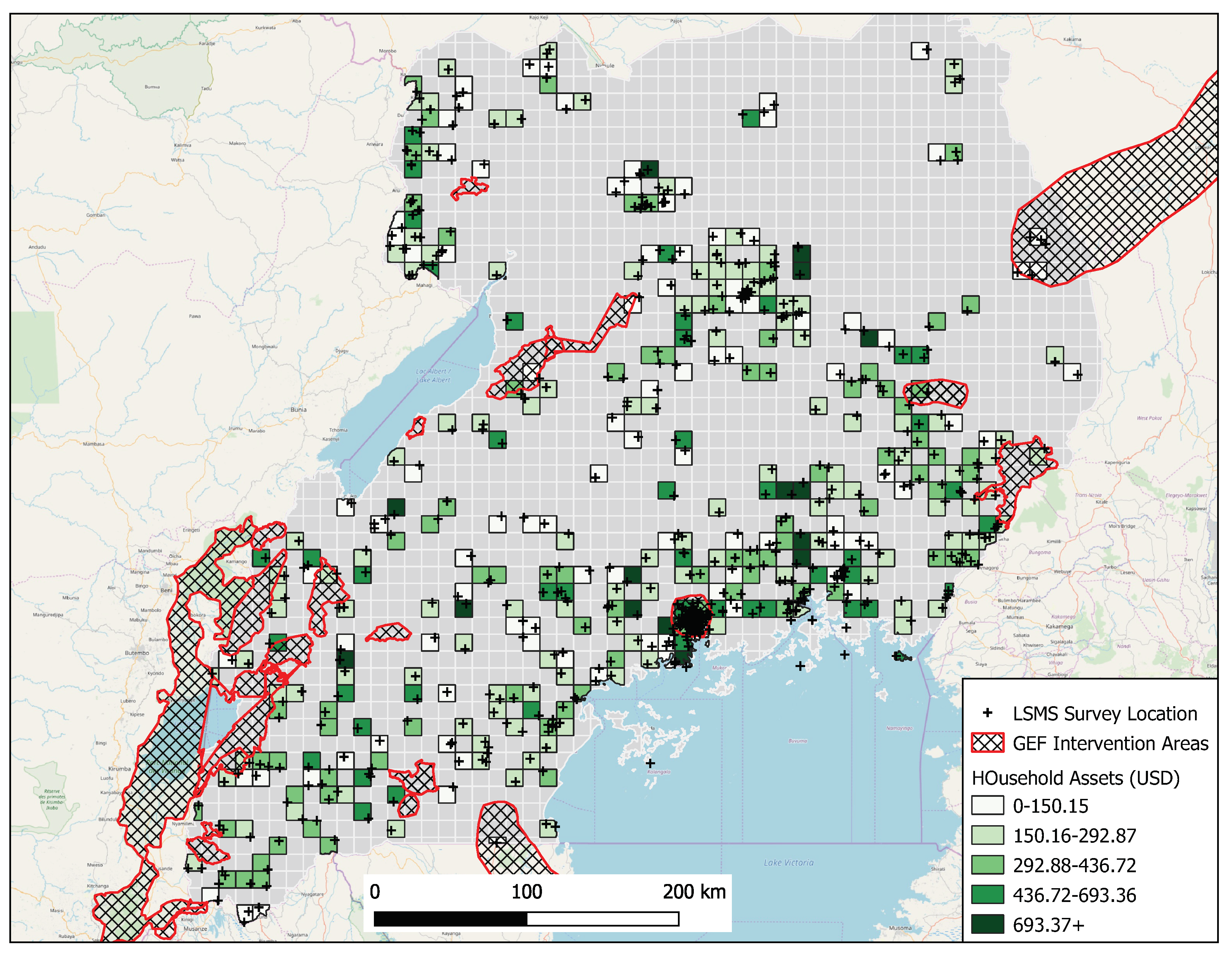
2.1. Data

This paper leverages a novel dataset of Global Environment Facility Sustainable Forest Management projects, represented by thousands of spatial boundaries defining areas of intervention. The analysis relies on a subset of 33 project locations in Uganda for which exact geographic boundaries are known, which can be seen outlined in red in Figure 1. Criteria for selection included projects which had direct implementations (i.e., activities that would impact the geographic region of intervention), intersection with Uganda, and project implementation dates before our baseline period of 2009. Projects include both small-scale projects implemented solely within Uganda, and regional-scale initiatives that were also inclusive of other projects within the region. As Figure 1 illustrates, the majority of projects analyzed here are along the border of Uganda, with a smaller number located in the interior. More generally, the GEF interventions we analyze here tend to be located in more remote areas (i.e., that do not overlap with the Living Standards Measurement Survey (LSMS) survey locations); this is likely reflective of GEF strategies which allocate aid to protected areas.

In addition to information on the geographic location of GEF SFM projects, data from the World Bank Living Standards Measurement Survey (LSMS) was used to estimate the outcome measure in this study—household assets. Collected in 2009 and 2011 within Uganda, the LSMS provides geographic latitude and longitude information on where household clusters were surveyed, accurate to within 5 km. In both surveys, an identical question was asked which is used in this analysis—“What is the total estimated value of all the assets owned by your household?”. In 2009, the LSMS surveyed 2960 households with an instrument that asked these questions; of these households, 2926 provided a response to this information along with geographic location information. In 2011, the LSMS surveyed 2497 households, of which 2316 households provided the same information. The locations of the 2009 surveys can be seen in Figure 1.

Geospatial covariates were retrieved and integrated into a standardized grid with a resolution of 10 km following the approach outlined in [33]; a full list of ancillary covariates is included in

Table 1. Ancillary data used in this analysis.

Feature	Source	Resolution
Nighttime Lights	Defense Meteorological Satellite Program (DMSP-OLS) [34]	1 km
	Visible Infrared Imaging Radiometer Suite (VIIRS) [35]	500 m
Road Networks	Global Roads Open Access Data Set (gRoads) [36]	1 km
Global Administrative Zones	geoBoundaries Administrative Zones [37]	Variable
Protected Areas	World Database of Protected Areas (WDPA) [38]	Variable
Population	Gridded Population of the World (GPW) [39]	1 km
Topography	Shuttle Radar Topography Mission (SRTM) [40]	500 m
Air Temperature	University of Delaware [41]	50 km
Precipitation	University of Delaware [41]	50 km
Land Cover	European Space Agency [42]	300 m
Land Surface Temperature	MODIS [43]	1 km
NDVI	NASA Long Term Data Record (LTDR) [44]	5 km

. This grid was used as our frame for analysis. The data collected from LSMS was aggregated to each cell to generate annual average measurements of household assets (2009 and 2011), and the distance between each cell and GEF SFM project was calculated; cells for which no household asset information existed were removed from the analysis. This resulted in the dataset used for analysis—each row being representative of a 10 square kilometer region across Uganda (as shown in Figure 1), containing measurements from the data sources in Table 1. Yearly measurements were derived where feasible, with average, max, and minimum yearly values being retrieved and saved. In temporally invariant cases such as roads, the distance to the nearest observation was calculated and assumed to be similar across the time periods surveyed (2009 and 2011).

2.2. Methods

In this section, we introduce Quasi-experimental Geospatial Interpolation (QGI). QGI is designed to mitigate two interrelated gaps in our current ability to model causal relationships with spatial data: (1) The challenge of spatial spillover, and (2) the challenge of selecting an appropriate distance band. We also briefly discuss the ways in which (3) QGI mitigates the possibility of omitted variables impacting the estimate of the treatment.

2.2.1. Key Methodological Concepts

Spillover

The challenge of spatial spillover is well summarized in [30]—specifically, the need to ensure that the units defined as “control” units (i.e., those that did not receive intervention) did not in any way benefit from the treatment. In a spatial context, this is a common challenge—i.e., if a village is a beneficiary of a sustainable farming training program, individuals from neighboring villages may travel to attend, or information from the program may naturally diffuse along social networks. This is also a challenge among treated units—i.e., a treatment effect may compound if more neighboring units are treated. The method presented here does not explicitly estimate this compounding effect, but such effects would be included in the overall treatment effect estimate (see [31] for a complete conversation of the challenges of SUTVA with spatial data).

Distance Bands

Interrelated to spillover is the challenge of selecting distance bands to distinguish between areas to be defined as “treated” or “untreated” (see, for example [30,32]). This challenge relates to the unknown nature of how interventions will diffuse over geographic space—i.e., if an animal clinic might benefit farmers within 10 or 50 km. Because this distance threshold is generally unknown, researchers are left to arbitrarily determine a threshold at which they anticipate no effect would be reasonable to expect; locations beyond this threshold are defined as “control” units. Arbitrarily choosing this distance can result in an increased likelihood of “p-score hacking”, or selecting for distances at which a desired effect is identified; varying this distance can result in bias due to the fact that a single unit can be defined as a “treated” unit in one analysis, and a “control” in another (see Figure 2 for an illustrative example of this challenge).

Omitted Variables

QGI extends a long history of research into quasi-observational research which seeks to enable causal attribution, specifically building on the “propensity score” matching approach [45,46]. This approach is intuitively described as one in which “twins” are identified, where one twin received a treatment and one did not. In such “twinned” studies, estimation for the purpose of causal attribution generally seeks to fit a model of a form similar to:

$$y_i=\beta 0+\theta \ast T_i+{\beta }_j\ast X_{i,j}$$

(1)

where $y_i$ is the outcome of interest (i.e., income), $\theta$ is the intervention (or treatment) effect on the outcome of interest for which an accurate estimate is desired, $T_i$ represents a binary indication of if unit of observation i received a given intervention, ${\beta }_j$ represent parameters we seek to fit to control for potential effects from sources other than the intervention j, and $X_{i,j}$ represents the value for unit of observation i for each control variable j. The most common approach to estimating $\theta$ is to construct a sample set in which all units that received an intervention ($T=1$) are matched one-to-one with units that did not receive an intervention ($T=0$), where matches are conducted to minimize differences along relevant dimensions (“twins”). Observations which are not a part of an optimally paired twin in the dataset are either removed (in one-to-one matching) or weighted (in many-to-one matching). This sample set is then used to estimate Equation (1). By only including twins in the analyses, the potential for omitted variable bias is reduced, as—in aggregate—it can be hypothesized that biases between twins due to unmeasured data will be similar in nature [45,46].

2.2.2. Quasi-Experiemental Geospatial Interpolation (QGI)

This paper introduces a new method for the estimation of causal impacts of an intervention using spatial data, Quasi-experimental Geospatial Interpolation (QGI). QGI provides a unique insight into the causal effect of interventions by allowing researchers to examine the spatial distance-decay of impacts (i.e., if a clinic has an effect only on the village it is located in, or also neighboring villages). QGI broadly mitigates two interrelated sources of bias: (1) The arbitrary selection of a distance threshold and (2) the possibility of spillover of interventions from treated to control locations.

Unlike other models used to examine causal impacts, QGI explicitly models the distance-decay function of the treatment estimate ($\theta$ in Equation (1)) through an iterative approach of changing the distance thresholds at which controls and treatments are demarcated (similar to the approach adopted by kriging-based spatial interpolation). It follows a three step process in which:

• Two hyperparameters are chosen:

  (a)

  The maximum distance ($\delta$) for which a treatment effect will be constructed.

  (b)

  The number of distance bands $\kappa$, with the geographic distance for each band denoted by ${\kappa }_i$.

• For each distance ${\kappa }_i$, we build a regression model following:

  (a)

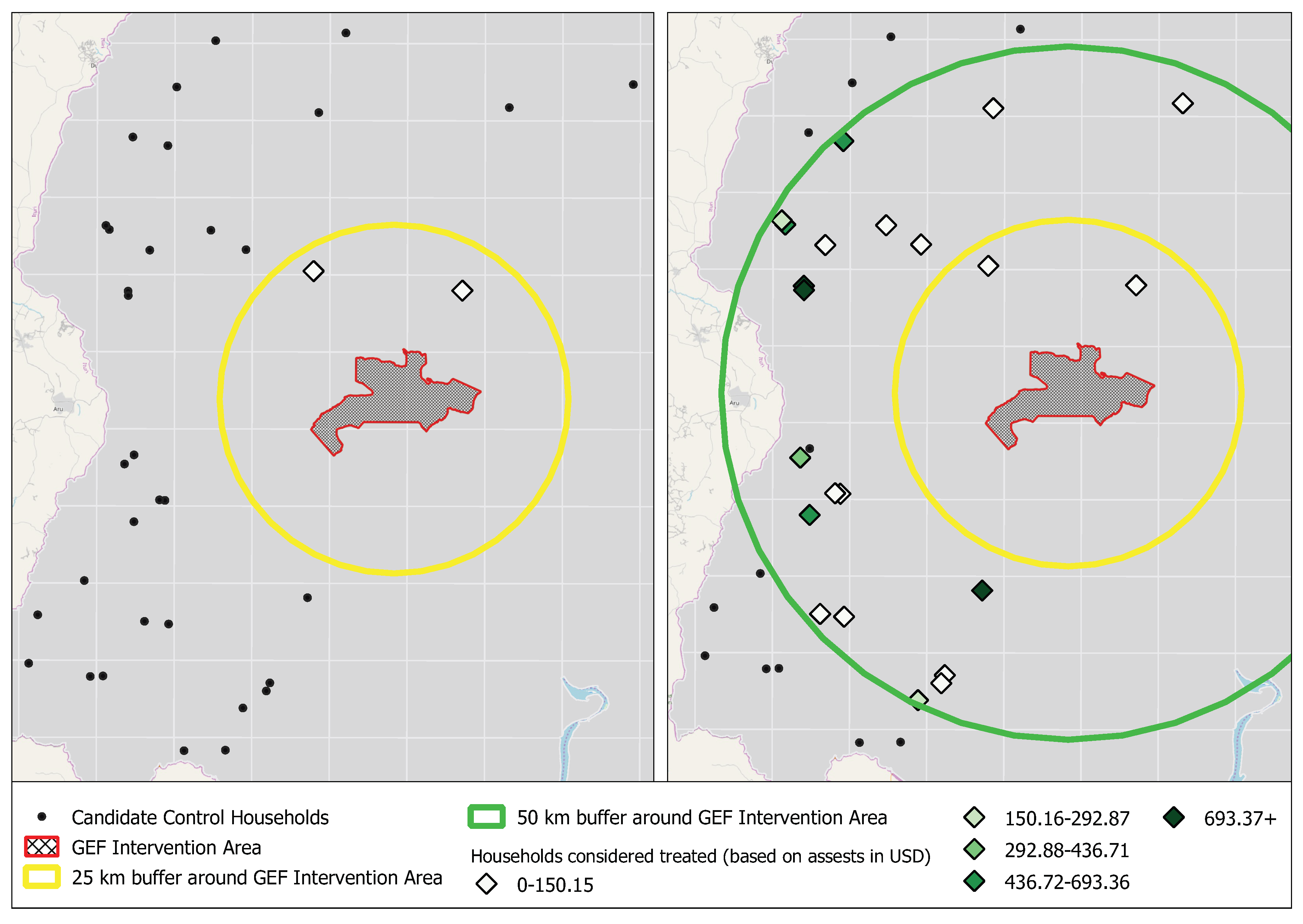
  All units of observation that are geographically closer to an intervention than the specified ${\kappa }_i$ are considered as "treated".

  (b)

  These units are matched with eligible control units that have a minimum distance away from an intervention site of $\delta$.

  (c)

  The quality of the matches (${\varphi }_i$) is calculated and recorded.

  (d)

  A regression model, similar to that in Equation (1), is estimated; both ${\theta }_i$ and the standard deviation ${\sigma }_i$ are recorded.

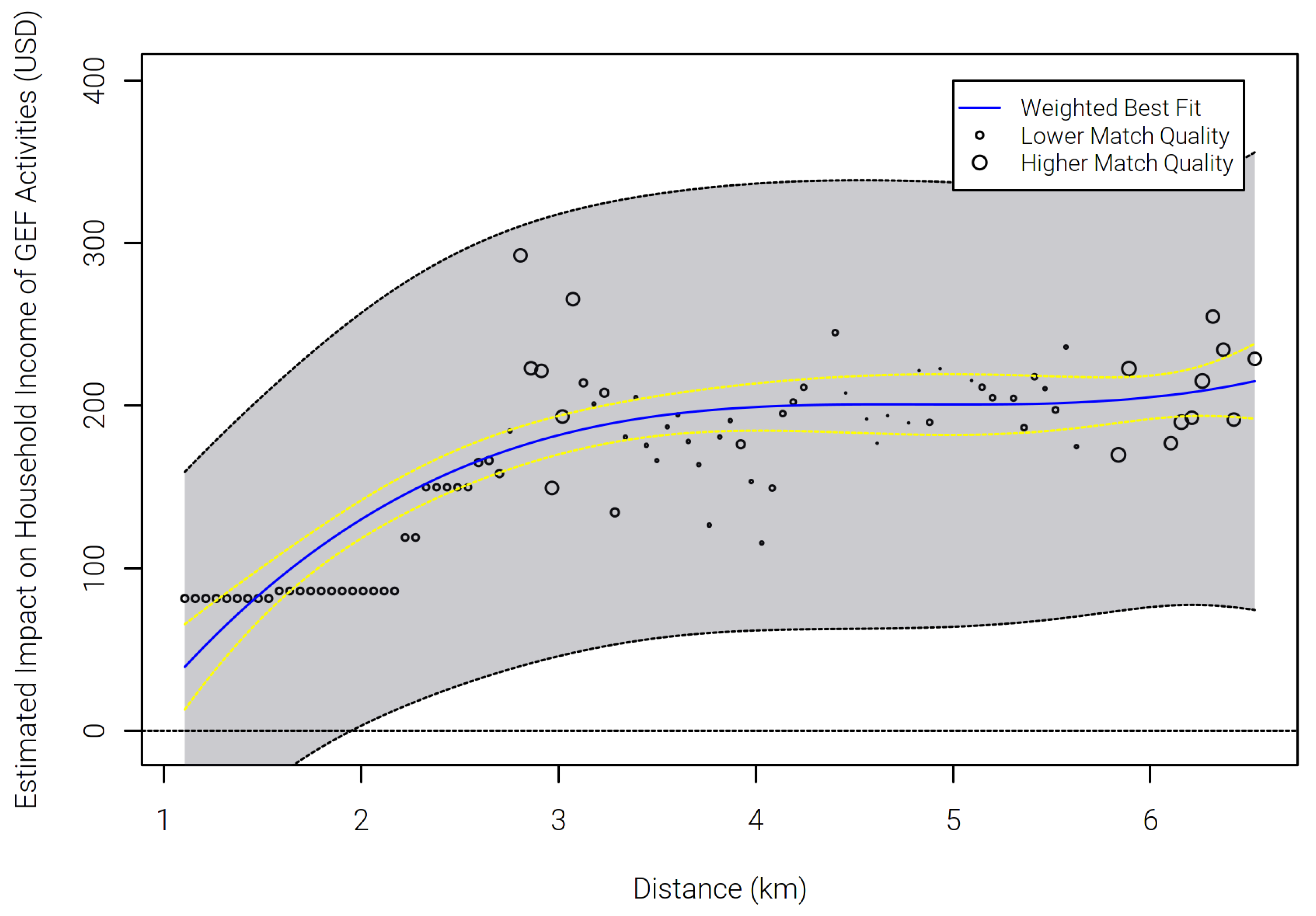
• After $\theta$ is recorded for all distance bands i, the relationship between distance and $\theta$ is estimated using a model of the users choice—i.e., spherical or polynomial, with a weighting approach in which distance bands with better match qualities (${\varphi }_i$) are given more weight. This is repeated for the standard deviation of the estimates ($\sigma$).

Following this approach, the relationship between distance, standard errors and estimated treatment effect can be visualized as illustrated in Figure 3.

2.2.3. Step 1—Hyperparameter Selection

Two hyperparameters must be selected to implement QGI—$\delta$, or the maximum distance for which an effect will be estimated, and $\kappa$, or the number of distance bands for which effects will be estimated (i.e., the resolution of the estimation). The range 0–$\delta$ is split into $\kappa$ equally-spaced distances, and represented for each distance as ${\kappa }_i$. For example, take the case of a researcher attempting to identify the impact of a training program in which a number of stakeholders were trained in a new irrigation strategy at Village A. If $\delta$ = 100 km, the implicit assumption would be that villages at least 100 km from Village A were not impacted by the training program in any way. If $\kappa$ is set to 3 in this case, a total of three distance bands would be saved: ${\kappa }_1=33.\overline{3}$, ${\kappa }_2=66.\overline{6}$, ${\kappa }_3=99.\overline{9}$. Of note, selecting a large $\delta$ value can help mitigate the probability that a study may be biased by spillover effects; however, this comes at the cost of increasing the probability quality matches cannot be found.

2.2.4. Step 2—Iterative Modeling

Step 2(a) Defining Treatment and Control for each Distance ${\kappa }_i$

For each value of $\kappa$, we define all units within distance ${\kappa }_i$ of an intervention as being “treated” (i.e., $T=1$ in Equation (1)). All units that are at least distance $\delta$ away from an intervention are identified as a control ($T=0$). This means that, for any given distance ${\kappa }_i$, we have a varying set of treated locations, and a static set of control locations they will be contrasted to.

Step 2(b) Matching “Twin” Treatment and Control Locations for each Distance ${\kappa }_i$

Our goal with the dataset constructed in step 2a is to contrast locations that were close (distance $<={\kappa }_i$) to an intervention to those that were at least distance $\delta$ away, but otherwise as similar as possible. To facilitate matching these “twin” locations, we estimate the likelihood that any unit was close to an intervention—referred to as a propensity score:

$$T_j={\beta }_0+{\beta }_k\ast X_{k,j}$$

(2)

where $T_j$ is a binary value indicating if location j is within distance ${\kappa }_i$ of an intervention site; ${\beta }_0$ is an intercept, ${\beta }_k$ is a fitted parameter value for covariate k, and $X_{k,j}$ is covariate k’s value for location j. An optimal parameterization of this model is identified through a logistic regression least squares approach, and the resultant propensity score predicted for every unit of observation j are saved as $P_j$. For every treated unit $T_j=1$, the single control unit $T_j=0$ with the most similar propensity score is identified and saved; a final dataset is then constructed that only contains these matches (unmatched cases are discarded). For more information on the mechanics of propensity score matching for causal inference we direct readers to [47].

Step 2(c) Calculating Match Quality for each Distance ${\kappa }_i$

Because matches are constructed iteratively across each distance, it is possible that some distances may have poor matches—i.e., there are not sufficient “twins”. To account for this, for each distance ${\kappa }_i$ a metric of match quality is calculated by taking the absolute value of the difference between the average propensity score (P) for treated and untreated cases:

$${\varphi }_i=\left|\left(\frac{P_j\ast T_j}{N}\right)-\left(\frac{P_j\ast \left|T_j-1\right|}{N}\right)\right|$$

(3)

This information is used in subsequent steps of QGI.

Step 2(d) Estimating θ for each Distance ${\kappa }_i$

After matching, constructing a new dataset which only includes matched cases, and recording the overall match quality $\varphi$, a linear regression model is fit:

$$y_j={\beta }_0+\theta \ast T_j+{\beta }_k\ast X_{k,j}$$

(4)

in which the ultimate goal is to estimate $\theta$ with a high degree of accuracy, using a maximum likelihood estimator. For each distance ${\kappa }_i$, the estimate of $\theta$ is saved as ${\theta }_i$, along with the standard error of the estimate ${\sigma }_i$.

2.2.5. Step 3—Estimating the Spatial Relationship between Distances ${\kappa }_i$ and Estimates ${\theta }_i$

Once all estimates of $\theta$ and $\sigma$ are constructed for each distance ${\kappa }_i$, we seek to establish the relationship between distance $\kappa$ and treatment effect $\theta$. While many methods for establishing the relationship between distance and another variable can be selected, here we implement a weighted third order polynomial. Weighting is accomplished by (a) dropping ($weight=0$) any matches that did not meet a threshold of match quality (in this case, a difference of 0.1), and (b) assigning more weight to the best relative matches using the estimation of match quality $\varphi$. Weighting is accomplished by adjusting the loss function from ordinary least squares to account for the weights provided by ${\varphi }_i$:

$$\sum {\varphi }_i\ast {(\widehat{{\theta }_i}-{\theta }_i)}^2$$

(5)

By repeating this process for the standard errors recorded in each model iteration (${\sigma }_i$), we can establish a predicted confidence interval around the polynomial trend line. By adding the model standard errors to the standard errors of the polynomial fit itself, we get a final envelope of possible errors for any given distance. In the results for the case study, Figure 3, the blue line indicates the 3rd order polynomial trend relating $\theta$ and distance; the area bracketed by yellow lines indicates the standard errors attributable to uncertainty regarding the estimate of this trend. The remainder of the grey region indicates standard errors attributable to the estimate of $\theta$ at each iteration i.

3. Results

This section introduces QGI using an illustrative case study in Uganda; the subsections here are reflective of each of the steps outlined in Section 2.2.

3.1. Step 1—Hyperparameter Selection for the Uganda Case Study

For this analysis, an upper distance bound of $\delta \approx$ 50 km was selected as a theoretical approximation of the maximum distance for which an effect could be detected (as the reader will see in later sections, the resultant estimate is—in this case—insensitive to this choice, as the maximum distance for which the data support conclusions is approximately 7 km). $\kappa$ was selected according to available computation, with 30 iterations being performed on each of 16 compute cores available (for a maximum index for $\kappa$ of 480 (${\kappa }_{480}$) (Initial exploration suggests that—for reasonably smooth surfaces—results are robust to this hyperparameter selection).

3.2. Step 2—Iterative Modeling for the Uganda Case Study

Within Uganda, we seek to contrast households surveyed by LSMS proximate to GEF projects to those that are not proximate. The goal of this contrast is to estimate the effect of GEF projects on household assets. In this iterative model fitting procedure, we contrast "close" households to "far" households, with the distance band defining "close" (${\kappa }_i$) increasing at each step until the maximum step $\delta$ is reached. A total of 480 distance thresholds tested, ranging from 0 to 50 km (see Section 3.1). The results of each of these 480 models are displayed in Figure 3, where a points place on the x-axis reflects distance threshold ${\kappa }_i$, and the y-axis position represents the estimate ${\theta }_i$. The size of each dot is representative of it’s relative match quality, ${\varphi }_i$ (see Section 2.2.4).

As an example, in the case of $i=41$, ${\kappa }_i\approx$ 5 km, and ${\theta }_{41}=209.41$. This can be interpreted as households within 5 km of GEF projects tend to have an income $209.41 higher than those at least 50 km away in Uganda, where 50 km is established by our selection of hyperparameter $\delta$ in Section 3.1.

3.3. Step 3—Distance Decay of the Observed Treatment Effects

The trend line and concomitant standard errors shown in Figure 3 represent the QGI estimate of the effect of GEF projects on household assets at distances ${\kappa }_i$. To fit this spatial model, first for each of our 480 iterations i we drop any cases that did not have sufficient matches to fit a model estimate, or did not have at least a certain threshold of match quality (in this case, a difference of 0.1). We then fit a 3rd-order polynomial trend, following the weighted model detailed in Section 2.2.4. As can be observed in Figure 3, all estimates suggest a positive impact on household assets; however, only for distances after approximately 2 km does statistically significant evidence exist. For these distances, an average effect of approximately $180 is detected.

4. Discussion and Conclusions

This paper sought to identify the relationship between the siting of GEF Sustainable Forest Management projects and changes in household assets in households proximate to those locations. By applying Quasi-experimental Geospatial Interpolation (QGI), we found robust and consistent evidence that the GEF had a positive impact on local household assets, to the order of approximately 180 USD between 2009 and 2011 (the survey years; Figure 3). While all distances estimated in this study suggested a positive impact, only distances greater than 2 km illustrated statistically significant positive impacts (see Figure 3); this is likely due to the relatively small number of cells proximate to GEF projects (making it challenge to establish a large enough N to detect significance at close distances). Insufficient evidence existed to examine impacts beyond approximately 7 km from GEF project intervention locations. We note evidence for an impact of approximately $180 is markedly consistent for distances between around 3 and 7 km from GEF projects.

A number of novel issues arose during the exploration of QGI. First, we note that previous approaches to Geospatial Impact Evaluation have relied heavily on re-using data as both control and treatment cases—i.e., as Figure 2 illustrates, by changing the distance at which you consider locations to have been effected by a treatment, you can end up classifying the same unit as “treated” in one iteration, and “control” in another. This, by it’s very nature, encourages “p-score hacking”, or searching through the data to find distance bands that support a particular finding. The proposed approach in this paper precludes this—by defining a maximum distance band, only units of observation that are beyond that distance can be included as potential counterfactual (“control”) units. This means that, no matter what distance band is chosen, the same set of controls are eligible for selection (and these same controls will never be treated as “treated” locations).

This approach has a second benefit of illustrating the impact of an intervention as a function of geographic distance. It is not reasonable to assume that an intervention that manifests spatially has no spatial pattern—i.e., a clinic implemented in one village will naturally impact neighboring villages more than those farther away. Past research—even that conducted by the authors (see [48])—has ignored this spatial decay pattern, leading to single estimates for entire regions. QGI provides researchers with an approach to overcome this shortfall.

QGI also offers the advantage of being deterministic—i.e., there is no simulation or random chance associated with the outcome. This not only promotes rapid computation (i.e., solutions can be arrived at in minutes on normal desktop hardware for reasonably sized datasets), but also promotes our ability to replicate findings.

Future Research

The use of quasi-experimental methods within the geographic literature is relatively new— little modeling has coupled, for example, the approaches discussed in this piece with more traditional spatial lag, error, or Durbin models. There are currently not approaches to solve for distance-decay patterns on a local basis—i.e., here we present a single global relationship, rather than estimating the likely decay pattern of any individual intervention. Further, there is an opportunity to integrate recent studies on spatial imprecision in measurements with QGI, or explore alternatives to propensity score matching that incorporate spatial effects. More broadly, there is limited literature on the relative accuracy of “Geospatial Impact Evaluation” as contrasted to more traditional a-spatial quasi-observational designs for causal identification; followup fieldwork could help provide such a contrast. Given the nascent nature of this subfield of study, the “sky is the limit” in terms of questions that can be asked.

Beyond the novel methodological research to be done, the substantive findings in this piece suggest that GEF SFM environmental interventions are linked to positive changes in household assets. However, significant research remains to be done on the specific nature of these linkages, and more broadly linkages between the environment and poverty. Such efforts could be implemented through qualitative surveys following a triangulation framework (see [49]) to validate findings and understand human perceptions on the ground. We further argue that replicating this study with more contemporary data could be of high value.

References

- Alpízar, F.; Ferraro, P.J. The Environmental Effects of Poverty Programs and the Poverty Effects of Environmental Programs: The Missing RCTs. World Dev. 2020, 127, 104783. [Google Scholar] [CrossRef]
- Lech, M.; Uitto, J.I.; Harten, S.; Batra, G.; Anand, A. Improving International Development Evaluation through Geospatial Data and Analysis. Int. J. Geospat. Environ. Res. 2018, 5, 13. [Google Scholar]
- Runfola, D.; Yishay, A.B.; Tanner, J.; Buchanan, G.; Nagol, J.; Leu, M.; Goodman, S.; Trichler, R.; Marty, R. A top-down approach to estimating spatially heterogeneous impacts of development aid on vegetative carbon sequestration. Sustainability 2017, 9, 409. [Google Scholar] [CrossRef]
- Buchanan, G.M.; Parks, B.C.; Donald, P.F.; O’donnell, B.F.; Runfola, D.; Swaddle, J.P.; Tracewski, L.; Butchart, S.H.M. The Local Impacts of World Bank Development Projects Near Sites of Conservation Significance. J. Environ. Dev. 2018, 27, 299–322. [Google Scholar] [CrossRef]
- Frumhoff, P. Monitoring the Environmental Impacts of USAID-Funded Activities to Conserve Biological Diversity; U. S. Agency for International Development: Washington, DC, USA, 1995. [Google Scholar]
- Christie, P. Observed and perceived environmental impacts of marine protected areas in two Southeast Asia sites. Ocean Coast. Manag. 2005, 48, 252–270. [Google Scholar] [CrossRef]
- Carpenter, R.A.; Maragos, J.E. How to Assess Environmental Impacts on Tropical Islands and Coastal Areas; Environment and Policy Institute: Honolulu, HI, USA, 1989. [Google Scholar]
- Qdais, H.A. Environmental impacts of the mega desalination project: The Red–Dead Sea conveyor. Desalination 2008, 220, 16–23. [Google Scholar] [CrossRef]
- Boocock, C.N. Environmental impacts of foreign direct investment in the mining sector in Sub-Saharan Africa. In Foreign Direct Investment and the Environment; OECD: Paris, France, 2002; p. 19. [Google Scholar]
- Ortolano, L.; Shepherd, A. Environmental impact assessment: Challenges and opportunities. Impact Assess. 1995, 13, 3–30. [Google Scholar] [CrossRef]
- Ryberg, B.T.; Dicks, M.R.; Hebert, T. Economic impacts of the conservation reserve program on rural economies. Rev. Reg. Stud. 1991, 21, 91–105. [Google Scholar]
- Bangsund, D.A.; Hodur, N.M.; Leistritz, F.L. Agricultural and recreational impacts of the conservation reserve program in rural North Dakota, USA. J. Environ. Manag. 2004, 71, 293–303. [Google Scholar] [CrossRef]
- Olatubi, W.O.; Hughes, D.W. Natural resource and environmental policy trade-offs: A CGE analysis of the regional impact of the Wetland Reserve Program. Land Use Policy 2002, 19, 231–241. [Google Scholar] [CrossRef]
- Siegel, P.B.; Johnson, T.G. Measuring the economic impacts of reducing environmentally damaging production activities. Rev. Reg. Stud. 1993, 23, 237–254. [Google Scholar]
- Henderson, D.; Tweeten, L.; Woods, M. A multicommunity approach to community impacts: The case of the conservation reserve program. Community Dev. 1992, 23, 88–102. [Google Scholar] [CrossRef]
- Hamilton, L.L.; Levins, R.A. Local Economic Impacts of Conservation Reserve Program Enrollments: A Sub-County Analysis. In Proceedings of the Sixth Joint Conference on Food, Agriculture and the Environment, Minneapolis, MN, USA, 31 August–2 September 1998. [Google Scholar]
- Cho, S.H.; Soh, M.; English, B.C.; Yu, T.E.; Boyer, C.N. Targeting payments for forest carbon sequestration given ecological and economic objectives. For. Policy Econ. 2019, 100, 214–226. [Google Scholar] [CrossRef]
- Campiche, J.; Dicks, M.; Shideler, D.; Dickson, A. Potential economic impacts of the managed haying and grazing provision of the Conservation Reserve Program. J. Agric. Resour. Econ. 2011, 36, 573–589. [Google Scholar]
- Swartzentruber, R. The Economic Consequences of Private Lands Conservation Using Conservation Easements in Colorado. Ph.D. Thesis, Colorado State University, Fort Collins, CO, USA, 2019. [Google Scholar]
- Hindery, D. Social and environmental impacts of World Bank/IMF-funded economic restructuring in Bolivia: An analysis of Enron and Shell’s hydrocarbons projects. Singap. J. Trop. Geogr. 2004, 25, 281–303. [Google Scholar] [CrossRef]
- Oldekop, J.A.; Sims, K.R.; Karna, B.K.; Whittingham, M.J.; Agrawal, A. Reductions in deforestation and poverty from decentralized forest management in Nepal. Nat. Sustain. 2019, 2, 421–428. [Google Scholar] [CrossRef]
- Naidoo, R.; Gerkey, D.; Hole, D.; Pfaff, A.; Ellis, A.M.; Golden, C.D.; Herrera, D.; Johnson, K.; Mulligan, M.; Ricketts, T.H.; et al. Evaluating the impacts of protected areas on human well-being across the developing world. Sci. Adv. 2019, 5, eaav3006. [Google Scholar] [CrossRef]
- Ferraro, P.J.; Hanauer, M.M. Quantifying causal mechanisms to determine how protected areas affect poverty through changes in ecosystem services and infrastructure. Proc. Natl. Acad. Sci. USA 2014, 111, 4332–4337. [Google Scholar] [CrossRef]
- Alix-Garcia, J.; McIntosh, C.; Sims, K.R.; Welch, J.R. The ecological footprint of poverty alleviation: Evidence from mexico’s oportunidades program. Rev. Econ. Stat. 2013, 95, 417–435. [Google Scholar] [CrossRef]
- McKinnon, M.C.; Cheng, S.H.; Dupre, S.; Edmond, J.; Garside, R.; Glew, L.; Holland, M.B.; Levine, E.; Masuda, Y.J.; Miller, D.C.; et al. What are the effects of nature conservation on human well-being? A systematic map of empirical evidence from developing countries. Environ. Evid. 2016, 5, 8. [Google Scholar] [CrossRef]
- Özerol, G.; Bressers, H.; Coenen, F. Irrigated agriculture and environmental sustainability: An alignment perspective. Environ. Sci. Policy 2012, 23, 57–67. [Google Scholar] [CrossRef]
- BenYishay, A.; Heuser, S.; Runfola, D.; Trichler, R. Indigenous land rights and deforestation: Evidence from the Brazilian Amazon. J. Environ. Econ. Manag. 2017, 86, 29–47. [Google Scholar] [CrossRef]
- Marty, R.; Goodman, S.; LeFew, M.; Dolan, C.; BenYishay, A.; Runfola, D. Assessing the causal impact of Chinese aid on vegetative land cover in Burundi and Rwanda under conditions of spatial imprecision. Dev. Eng. 2019, 4. [Google Scholar] [CrossRef]
- Jain, M. The Benefits and Pitfalls of Using Satellite Data for Causal Inference. Rev. Environ. Econ. Policy 2020, 14, 157–169. [Google Scholar] [CrossRef]
- Buchanan, G.M.; Parks, B.C.; Donald, P.F.; O’donnell, B.F.; Runfola, D.; Swaddle, J.P.; Tracewski, L.; Butchart, S.H.M. The Impacts of World Bank Development Projects on Sites of High Biodiversity Importance; Technical Report; AidData at William & Mary: Williamsburg, VA, USA, 2016. [Google Scholar]
- Corrado, L.; Fingleton, B. Where is the economics in spatial econometrics? J. Reg. Sci. 2012, 52, 210–239. [Google Scholar] [CrossRef]
- Bunte, J.; Desai, H.; Gbala, K.; Parks, B.; Runfola, D.M. Natural resource sector FDI, government policy, and economic growth: Quasi-experimental evidence from Liberia. World Dev. 2018, 107, 151–162. [Google Scholar] [CrossRef]
- Goodman, S.; BenYishay, A.; Lv, Z.; Runfola, D. GeoQuery: Integrating HPC systems and public web-based geospatial data tools. Comput. Geosci. 2019, 122, 103–112. [Google Scholar] [CrossRef]
- Hsu, F.; Baugh, K.E.; Ghosh, T.; Zhizhin, M.; Elvidge, C.D. DMSP-OLS radiance calibrated nighttime lights time series with intercalibration. Remote Sens. 2015, 7, 1855–1876. [Google Scholar] [CrossRef]
- Elvidge, C.D.; Baugh, K.; Zhizhin, M.; Hsu, F.C.; Ghosh, T. VIIRS night-time lights, 2017. Int. Remote Sens. 2017, 38, 5860–5879. [Google Scholar] [CrossRef]
- Center for International Earth Science Information Network-CIESIN-Columbia University, Information Technology Outreach Services-ITOS-University of Georgia. Global Roads Open Access Data Set, Version 1 (gROADSv1); NASA Socioeconomic Data and Applications Center (SEDAC): Palisades, NY, USA, 2013. [Google Scholar] [CrossRef]
- Runfola, D.; Anderson, A.; Baier, H.; Crittenden, M.; Dowker, E.; Fuhrig, S.; Goodman, S.; Grimsley, G.; Layko, R.; Melville, G.; et al. geoBoundaries: A Global Database of Political Administrative Boundaries. PLoS ONE 2020. [Google Scholar] [CrossRef]
- Bingham, H.C.; Bignoli, J.D.; Lewis, E.; MacSharry, B.; Burgess, N.; Visconti, P.; Deguignet, M.; Misrachi, M.; Walpole, M.; Stewart, J.; et al. Sixty years of tracking conservation progress using the World Database on Protected Areas. Nat. Ecol. Evol. 2019, 3, 737–743. [Google Scholar] [CrossRef] [PubMed]
- Balk, D.L.; Deichmann, U.; Yetman, G.; Pozzi, F.; Hay, S.I.; Nelson, A. Determining global population distribution: Methods, applications and data. Adv. Parasitol. 2006, 62, 119–156. [Google Scholar] [PubMed]
- Rodriguez, E.; Morris, C.S.; Belz, J.E. A global assessment of the SRTM performance. Photogramm. Eng. Remote Sens. 2006, 72, 249–260. [Google Scholar] [CrossRef]
- Matsuura, K.; Willmott, C.J. Terrestrial Air Temperature & Precipitation: 1900–2014 Gridded Monthly Time Series. 2015. Available online: http://climate.geog.udel.edu/~climate/html_pages/download.htm (accessed on 10 March 2020).
- Lesiv, M.; Fritz, S.; McCallum, I.; Tsendbazar, N.; Herold, M.; Pekel, J.F.; Buchhorn, M.; Smets, B.; Van De Kerchove, R. Evaluation of ESA CCI Prototype Land cover Map at 20m. 2017. Available online: http://pure.iiasa.ac.at/id/eprint/14979/ (accessed on 10 March 2020).
- Wan, Z. MODIS Land Surface Temperature Products Users’ Guide; Institute for Computational Earth System Science, University of California: Santa Barbara, CA, USA, 2006. [Google Scholar]
- Nagol, J.R.; Vermote, E.F.; Prince, S.D. Effects of atmospheric variation on AVHRR NDVI data. Remote Sens. Environ. 2009, 113, 392–397. [Google Scholar] [CrossRef]
- Ho, D.E.; Imai, K.; King, G.; Stuart, E.A. MatchIt: Nonparametric preprocessing for parametric causal inference. J. Stat. Softw. 2011. Available online: http://gking.harvard.edu/matchit (accessed on 19 March 2020). [CrossRef]
- Imbens, G.W.; Rubin, D.B. Rubin causal model. In Microeconometrics; Palgrave Macmillan: London, UK, 2010; pp. 229–241. [Google Scholar]
- Zhao, J.; Runfola, D.M.; Kemper, P. Quantifying Heterogeneous Causal Treatment Effects in World Bank Development Finance Projects. In Joint European Conference on Machine Learning and Knowledge Discovery in Databases; Technical Report; Springer: Cham, Switzerland, 2017. [Google Scholar]
- Marty, R.; Dolan, C.; Leu, M.; Runfola, D. Taking the Aid Debate to the Sub-National Level: Impact and Allocation of Foreign Health Aid in Malawi. BMJ Global Health 2017, 2, e000129. [Google Scholar] [CrossRef]
- Carugi, C. Experiences with systematic triangulation at the Global Environment Facility. Eval. Prog. Plann. 2016, 55, 55–66. [Google Scholar] [CrossRef]