Finite Element Simulation of Multi-Slip Effects on Unsteady MHD Bioconvective Micropolar Nanofluid Flow Over a Sheet with Solutal and Thermal Convective Boundary Conditions

Abstract

In this article, the intention is to explore the flow of a magneto-hydrodynamic (MHD) bioconvective micro-polar Nanofluid restraining microorganism. The numerical solution of 2-D laminar bioconvective boundary layer flow of micro-polar nanofluids are presented. The phenomena of multi-slip, convective thermal and Solutal boundary conditions have been integrated. A system of non-linear partial differential equations are transformed into the system of coupled nonlinear ordinary differential equations by applying appropriate transformations, the transformed equations are then solved by applying the variational finite element method (FEM). The fascinating features of assorted velocity parameter, microrotation, temperature, microorganism compactness, solutal and nanoparticles concentration have been inspected. The rate of heat transfer, the skin friction coefficient, couple stress and Sherwood number for microorganisms have also been discussed graphically and numerically. The investigations illustrated that increase in material parameters causes a reduction in microorganism compactness, concentration and temperature. As a result of enhancement in the unsteadiness parameter, the fluid velocity, concentration of microorganisms and the temperature are observed to be declines. Energy and microorganism compactness profile affected by the improvement in the buoyancy ratio parameter. As the improvement in results of buoyancy ratio parameter effects on improvement in the energy and the microorganism compactness profile while the velocity profile is condensed. In the end, rationalized convergence of the finite element solution has been inspected; the computations are found out via depreciating the mesh size.

1. Introduction

The transfer of heat is the basic feature of the gigantic appliance through applications. The heat transfer depends on the thermal conductivity of the functioning fluids as measures up to the aptitude of thermal appliances and the structure. Nanofluids are deferments of nanoparticles in fluids that demonstrate the momentous enrichment of their properties at retiring nanoparticle concentrations. There are numerous publications on nanofluids that concerned to understand their behavior so that it can be employed wherever the straight heat transfer enrichment is dominant as in various industrial applications, nuclear reactors, transportation, electronics as well as biomedicine and food. nanofluid has been testified, where the heat transfer can be condensed or increased. Wen [1] represents about the inadequate considerate of the construction and mechanism of nanofluids and their applications. Exploration of nanofluids has proceeded quickly since its enhanced thermal conductivity was first reported about a decade ago, though much controversy and inconsistency have been reported. Yang et al. [2] examined the viability of the new application, the stable TiO${}_2$ nanofluids constructed to examine the formaldehyde and total volatile organic compounds (TVOC) distillation as well as sterilization. They also investigated the heat recovery characteristics of nanofluids by testing the gas-liquid aerated heat transfer behavior. The learning of magnetohydrodynamics plays an imperative role as it has importance in industry and much another flow phenomenon. From the last few decades, the endeavor to explore fluid physics at the nano and micro scales has improved. The fluid flow in the micro-scale is different from that on the macroscale. Areas of biological, microcirculation, molecular machinery, atherogenesis and micro-fluidics have motivated researchers to work on micro-scale phenomena in the field of fluid mechanics. It is desirable to investigate the large scale applications of non-Newtonian fluids in different industries, such as molten plastics, imitation fibers, nuclear desecrate disposal, slurries, transpiration cooling and petroleum tanks, and their characteristic performance. The heat transfer, resolute by the thermal radiation, has huge applications in diverse scientific processes, nuclear power plants, space vehicles, gas turbines, satellites, comprising missiles and in many impulsive devices for jets. Bio-convection arrangement which is a common phenomenon, they generally take place due to up-swimming of germs (tiny living organism like as microbes, microorganisms that are observable in microscopes) that is slightly impenetrable. By up-swimming, the top portion of the liquid layers of postponement becomes too dense. Due to the assembly of microorganisms, it happens to wobbly. In the geophysical phenomenon, Thermo bio-convection plays an imperative role, resembling in the phenomenon of thermopiles in which motile microorganisms roam warm springs. Moreover in the field of oil convalescence enhances by microbial. In oil-bearing layers are further microorganisms and nutrients to systematize permeability discrepancy. Bio-convective flows with magnetohydrodynamics (MHD) have quite a lot of applications in different fields such as hyperthermia, Treatment of several arterial syndromes, the illustration of copper wires and diminution of blood in surgeries and many other fields. A Casson fluid has an inestimable thickness at zero rates of shear and has zero thickness at an inestimable rate of shear and relent stress in which no flow happens. Therefore, Casson-fluid has to be described as shear contraction fluid/pseudoplastic fluid. The flow features of blood can precisely explain by Casson fluid at small shear rates. Pradhan et al. [3] Investigation are conceded out for free convective flow of an electrically executed micropolar fluid over an absorbent able stretching sheet in the existence of porous medium. Sharada and Shankar [4] numerically investigated the consequences of Soret/Dufour, chemical reaction, thermal radiation on the fluid flow, mass and heat transfers of Casson fluid through the exponentially elongating surface. Moradikazerouni [5] scrutinized the numerical heat transfer and thermal deformation of a micro-channel heat sink with various ingress channels. Pushpalatha et al. [6] investigate that the thermos-diffusion and thermos-diffusion impact on Casson fluid over an unsteady stretching surface with thermal radiation and magnetic field. Also, it described that Casson-parameter and unsteadiness parameter contains the proclivity to disparage the velocity distribution. Vo et al. [7] represents the influences of numerous shapes of γ-AlOOH nanoadditives (i.e., cylindrical, brick, blade and platelet) on the fluid flow and the heat transfer aspects of a sinusoidal grooved channel. Also, scrutinized the impact of nanoadditive fraction and Reynolds number on the performance of nanofluid in the grooved. Ullah et al. [8] analyzed the buoyancy-driven unsteady flow of Casson nanofluid. Also, see the consequences of Brownian motion and thermophoresis on the flow fields that are deliberated in the existence of a magnetic field. Uddin et al. [9] deliberated about free convective boundary layer flow of nanofluid over a penetrable vertical plate tinplate porous medium along with thermal convective boundary conditions. Alsarraf et al. [10] represents that a two-phase mixture model is used to discuss the turbulent boehmite alumina nanofluid inside a double-pipe heat exchanger and appraise the effect of nanoparticle concentration and Reynolds number on the heat exchanger performance. Moradikazerouni [11] investigated the influence of heat sink thermal demonstration and of the environmental parameters on the heat sink’s stability against thermal stress, which are important for manufacturers’ targets. They also inspected the effects of parameters on heat the transfer rate from the surface of the heat sink. Ranjbarzadeh et al. [12] scrutinized experimentally that the improvement of thermal properties of deionized water (base fluid), stability and the thermal conductivity of the silica-water nanofluid. The thermal conductivity of the organized nanofluid has been experimentally inspected in the wide range of temperatures and solid volume fractions. Naseem et al. [13] investigated the study of MHD bio-convection non-Newtonian nanofluid flow over a stretching sheet and conclude that, the motile concentration profile compact for greater Péclet and bio-convection Lewis number. It is acknowledged that in space, the gravity effect is decreased as a result of both the thermal buoyancy consequence and solutal buoyancy consequence are also decreased. The g-jitter/lingering accelerations originate commencing the diversity of resources like crew movements, perfunctory vibrations like as propels, motors, spacecraft exercises, distinctive drag and the gradient of earth’s weightiness [14]. The movement of macroscopic convective fluid flow due to the compactness is greater than water, which is entitled bio-convection [15,16]. It is valuable in fuel cell machinery, biodiesel fuels, bio-reactors, bio-micro organisms and gas-bearing, and so forth. The advantages of summing up the motile microorganisms to nanoparticles are enhancing the mass transporting and perk up the constancy of nanofluid. Dissimilar bio-convection nanofluid sculpts were studied based on various kinds of microorganisms and in the motion system of the fluid. Kuznetsov [17] examined that a horizontal layer of nanofluid that restrain gyro tactic microorganisms, then the particles may either lift up or sadden critical Rayleigh numbers, while the microorganisms have always subverting effect. In view of oxytactic motile microorganisms, bio-convection in nanofluid drenched in porous media, he also notorious that the nanofluid constancy is stated by nanoparticles allocation, compactness stratification stimulated by a perpendicular temperature gradient, by up-swimming of oxytactic microorganisms. Reference [18] revealed that the existence of oxytactic microorganisms reduces the nanofluid postponement consistency and eradicates the oscillatory inconsistency as compare to non-oscillatory inconsistency. Recently, Rahman et al. [19] investigated that the hydro-magnetic multi slip flow of water-based nanofluid through a wedge along with convective surface in the subsistence of heat production or assimilation. Ibrahim and Shankar [20] evaluated the magneto-hydrodynamic boundary layer flow and the heat transfer of nanofluid past through penetrable stretching sheet using thermal, velocity and solutes slip boundary conditions. Ma et al. [21] scrutinized that the heat transference of alumina/water nanofluid in a square inclusion through an inclined magnetic field and also investigate the impact of Ra, Hartman number, magnetic field angle, enclosure angle, the volume fraction of nanoadditives and aspect ratio on the heat transfer. Das [22] obtained a very important numerical inquiry on the convective heat transfer recital of nanofluids over a penetrable stretching surface in the existence of thermal buoyancy, partial slip and internal heat production/fascination. Abbas et al. [23] calculated the impacts of radiation in the existence of the same magnetic field for the nanofluid on a curled stretching surface by assimilating the consequences of slip. In recent times, Makinde et al. [24] have seen numerically the radiation consequences on chemically reacting MHD nanofluid manipulated by the heat source/sink and also illustrated the radiation effects in collective heat and mass relocating investigation for mixed convection flow in excess of the perpendicular plane with radiation and chemical reaction. Aziz et al. [25] using the Buongiorno model [26] deliberated the boundary layer flow through a porous medium crammed with nanofluid and gyrotactic microorganism. They give a correspondence solution and illustrated that the influences of the dimensionless parameters on the behavior of motile microbes. Several experimental consequences have given the verifications to support the slip condition [27]. In recent publications [28,29,30,31,32,33] investigated the significant significance of nanofluids in distinctive types of microsystems. The fluid motion of macroscopic convective flow caused by density, which is vaguely higher than water called bio-convection. It is valuable in fuel cell equipment, bio-micro systems, bio-reactors, bio-diesel fuels and gas-bearing sedimentary, and so forth. The reimbursement of accumulation motile microorganisms to nanoparticles is to improve the mass transfer and get better the stability of nanofluid. Different bio-convection nanofluid models were deliberated on the basis of different categories of microorganisms and the directional motion system of the fluid.

Inspired by the above literature, and in the applications of numerous areas that have been discussed, an investigation of the impact of multi-slip and solutal boundary conditions on MHD unsteady bioconvective micropolar nanofluid restraining gyrotactic microorganism, heat and mass transfer effect over a stretching/shrinking sheet (which have not been discussed before) was carried out. The main intent of contemporary study is the analysis of the radiative MHD Micropolar nanofluid having micro-organisms. Furthermore, the article is made more fascinating by the usage of solutal and thermal boundary conditions with radiative heat flux in the unsteady Micropolar nanofluid fluid flow over the stretching sheet. The deportment of existing parameters is demonstrated graphically through an appropriate discussion. After that, suitable similarities have been used for transformation; the governing non-linear partial differential equations are composed in a non-linear system of ordinary differential equations (ODEs). The resulting system of non-linear ODEs has been solved numerically with a proficient and authenticated variational finite element method (FEM) along with the boundary conditions. The influences of various parameters are studied graphically. Furthermore, the graphical narration of Nusselt number and microorganism flux is accessible and the skin friction behavior and also the impact of different parameters of the flow is numerically inspected. After that, the numerical comparison of the existing results has been presented and discussed with graphs. In view of this study, transient flow with slip effects with the existence of mixed convection and chemical reaction on the sheet/disk can be observed.

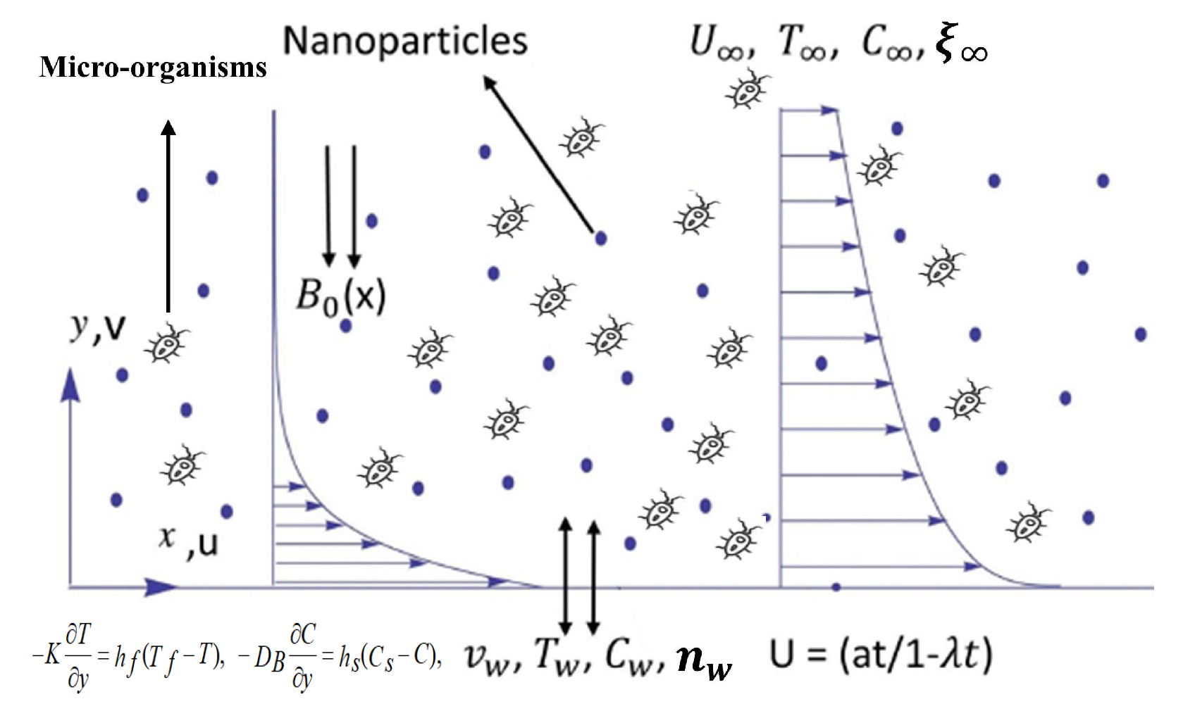
2. Problem Description

Consider the 2-D unsteady boundary layer MHD bioconvective flow of an incompressible fluid and micropolar nanofluid viscous flow over an electrically conducted stretching/shrinking sheet has been considering for exploration. The solutal and slip impacts have also been integrated. We made a decision with the Cartesian system with the purpose that the measurement of the sheet would be taken with x-axis, y-axis, and the x-axis would be chosen beside the stretching sheet, the vertical axis would be perpendicular to the surface as given in Figure 1. $U(x,t)=ax/(1-\lambda t)$ is the non-uniform velocity of sheet, since a is the stretching rate along x-axis but $\lambda t$ is positively constant as by condition $\lambda t<1$. The uniform magnetic field is supposed to be a function of distance from the origin, where $B_0$ is the potency of the magnetic field and is applied along the direction of the positive y-axis. The magnetic Reynolds numeral is very small as compared to the induced magnetic field. The free stream temperature is supposed to be $T_{\infty }$, the free mass concentration is as $C_{\infty }$ and the concentration of microorganisms is $n_{\infty }$. The governing equations for flow can be expressed (Ullah et al. [8]).

$$\frac{\partial u}{\partial x}+\frac{\partial v}{\partial y}=0,$$

(1)

$$\frac{\partial u}{\partial t}+u\frac{\partial u}{\partial x}+v\frac{\partial u}{\partial y}=({\nu }_f+\frac{k_f}{{\rho }_f})\frac{{\partial }^{2}u}{\partial y^2}+\frac{k_f}{{\rho }_f}\frac{\partial N}{\partial y}-\frac{\sigma B_0^{2}u}{{\rho }_f}$$

$$+\frac{1}{{\rho }_f}[(1-C_{\infty })(T-T_{\infty }){\rho }_f{\beta }_g-({\rho }_p-{\rho }_f)(C-C_f)g-(n-n_{\infty })({\rho }_m-{\rho }_f){\gamma }^{*}g]$$

(2)

$$\rho j(\frac{\partial N}{\partial t}+u\frac{\partial N}{\partial x}+v\frac{\partial N}{\partial y})={\gamma }_f(\frac{{\partial }^{2}N}{\partial y^2})-{\kappa }_f(2N+\frac{\partial u}{\partial y})$$

(3)

$$\frac{\partial T}{\partial t}+u\frac{\partial T}{\partial x}+v\frac{\partial T}{\partial y}=\alpha (1+\frac{16T_{\infty }^3{\sigma }^{*}}{3k^{*}\kappa })\frac{{\partial }^{2}T}{\partial y^2}+\tau D_B\frac{\partial C}{\partial y}\frac{\partial T}{\partial y}+\tau \frac{D_T}{T_{\infty }}{(\frac{\partial T}{\partial y})}^2+\frac{\sigma B_0^{2}u}{{(\rho c_p)}_f}$$

(4)

$$\frac{\partial C}{\partial t}+u\frac{\partial C}{\partial x}+v\frac{\partial C}{\partial y}=D_B\frac{{\partial }^{2}C}{\partial y^2}+\frac{D_T}{T_{\infty }}\frac{{\partial }^{2}T}{\partial y^2}$$

(5)

$$\frac{\partial n}{\partial t}+u\frac{\partial n}{\partial x}+v\frac{\partial n}{\partial y}+b{W}_c\frac{\partial }{\partial y}(\frac{n}{\mathsf{\Delta }c}\frac{\partial C}{\partial y})=D_m\frac{{\partial }^{2}n}{\partial y^2},$$

(6)

where x and y are the co-ordinates with the x and y-axis, u is the velocity components along the x-axis and v with the y-axis and $\alpha$, $\nu$, $\sigma$, are the thermal diffusivity, kinetic viscosity, and electrical conductivity, respectively. And symbolizes that ${\rho }_f$ is nanofluid density, ${\rho }_p$ is nanoparticle density, ${\rho }_m$ is microorganism density and g is the gravity. The temperature is T, C is the solutal concentration; n is the concentration of microorganisms and $T_0$, $C_0$ and $n_0$ represents the reference temperature, reference concentration of nanoparticles and reference concentration of the microorganisms, respectively. $T_w$, $C_w$, $n_w$ and $T_{\infty }$, $C_{\infty }$, $n_{\infty }$ symbolizes the surface temperature, the concentration of nanoparticles, the concentration of the microorganisms, free stream temperature, compactness of nanoparticles and the concentration of microorganisms, respectively, and N represents the angular velocity. $D_M$ is the molecular diffusivity; $D_T$ is the thermal diffusivity, $D_B$ is the Brownian diffusivity, in Equation (3), viscosity ${\gamma }_f$, expressed as (${\mu }_f+\frac{{\kappa }_f}{2})j$ where ${\kappa }_f$ is the eddy viscosity and Rosseland eradicative heat flux is $q_r$, which is delineated by $q_r=-(\frac{4{\sigma }^{*}}{3{\kappa }^{*}}\frac{\partial T^4}{\partial y})j$ wherever ${\sigma }^{*}$ is Stefan-Boltzmann numeral and ${\kappa }^{*}$ is the mean assimilation coefficients. And in Equation (6), n is the compactness of microorganisms, the chemotaxis invariable is b, $W_c$ is velocity cell swimming. The boundary conditions for the mathematical model are followed as (see [8]):

$$\begin{array}{c}u=U(x,t)+U_{slip},v=v_w,-\kappa \frac{\partial T}{\partial y}=h_f(T_f-T),-D_B\frac{\partial C}{\partial y}=h_s(C_s-C),\end{array}$$

$$\begin{array}{c}n=n_w(x,t)+n_{slip},N=-m\frac{\partial u}{\partial y}asy=0\end{array}$$

(7)

$$\begin{array}{c}uandN\to 0,T\to T_{\infty },C\to C_{\infty },n\to n_{\infty },asy\to \infty ,\end{array}$$

(8)

wherever the injection/suction velocity is $v_w=v_0/\sqrt{x}$, $T_w(x,t)$ is the temperature of the sheet and $C_w(x,t)$, $E_w(x,t)$ are concentrations at surface of the below form [34]:

$$T_w(x,t)=T_{\infty }+T_0\left(\frac{ax}{2\nu {(1-\lambda t)}^2}\right)$$

$$C_w(x,t)=C_{\infty }+C_0\left(\frac{ax}{2\nu {(1-\lambda t)}^2}\right)$$

$$n_w(x,t)=n_{\infty }+n_0\left(\frac{ax}{2\nu {(1-\lambda t)}^2}\right),$$

where $T_0$, $C_0$ and $n_0$ are the reference temperature, solutal concentration and bio-convection concentration respectively, such that $0\le T_0\le T_w$, $0\le C_0\le C_w$ and $0\le n_0\le n_w$, with this above phrases are legitimate if $(1-\lambda t)>0$.

Generally, the stream function $\mathsf{\Psi }$ is defined as $u=\frac{\partial \mathsf{\Psi }}{\partial y}$ and $v=-\frac{\partial \mathsf{\Psi }}{\partial x}$ which satisfies the equation of continuity automatically. Following are the similarity transformations to solve the above Equations (see [34,35,36]):

$$\eta =\sqrt{\frac{a}{\nu (1-\lambda t)}}y,\psi =\sqrt{\frac{a\nu }{(1-\lambda t)}}xf(\eta ),N=\sqrt{\frac{a^3}{\nu {(1-\lambda t)}^3}}xg(\eta ),\theta (\eta )=\frac{T-T_{\infty }}{T_w-T_{\infty }},$$

$$\varphi (\eta )=\frac{C-C_{\infty }}{C_w-C_{\infty }}\xi (\eta )=\frac{n-n_{\infty }}{n_w-n_{\infty }}.$$

(9)

In view of above similarity transformations Equation (9), PDEs from (1)–(6) transform into the following system of nonlinear ordinary differential equations (ODEs):

$$(1+K)\frac{d^{3}f}{d{\eta }^3}-{(\frac{df}{d\eta })}^2+f\frac{d^{2}f}{d{\eta }^2}+K\frac{dg}{d\eta }-M\frac{df}{d\eta }+\lambda (\theta -N_r\varphi -R_b\xi )-\sigma (\frac{\eta }{2}\frac{d^{2}f}{d{\eta }^2}+\frac{df}{d\eta })=0,$$

(10)

$$(1+\frac{K}{2})\frac{d^{2}g}{d{\eta }^2}+f\frac{dg}{d\eta }-g\frac{df}{d\eta }-K(2g+\frac{d^{2}f}{d{\eta }^2})-\sigma (\frac{\eta }{2}\frac{dg}{d\eta }+\frac{3}{2}g)=0$$

(11)

$$(1+\frac{4}{3}{R}_d)\frac{1}{P_r}\frac{d^2\theta }{d{\eta }^2}+f\frac{d\theta }{d\eta }-\theta \frac{df}{d\eta }+M{E}_c{(\frac{df}{d\eta })}^2+Nb\frac{d\varphi }{d\eta }\frac{d\theta }{d\eta }+Nt{(\frac{d\theta }{d\eta })}^2-\sigma (\frac{\eta }{2}\frac{d\theta }{d\eta }+2\theta )=0$$

(12)

$$\frac{d^2\varphi }{d{\eta }^2}-S_c(\frac{df}{d\eta }\varphi -f\frac{d\varphi }{d\eta })+\frac{N_t}{N_b}\frac{d^2\theta }{d{\eta }^2}-\sigma (\frac{\eta }{2}\frac{d\varphi }{d\eta }-2\varphi )S_c=0$$

(13)

$$\frac{d^2\xi }{d{\eta }^2}-Lb(\frac{df}{d\eta }\xi -f\frac{d\xi }{d\eta })-Pe[\frac{d^2\xi }{d{\eta }^2}(\xi +\mathsf{\Omega })+\frac{d\xi }{d\eta }\frac{d\varphi }{d\eta }]-\sigma (\frac{\eta }{2}\frac{d\xi }{d\eta }+2\xi )Lb=0,$$

(14)

for the above problem, the transformed boundary conditions are:

$$f(0)=f_w,\frac{df(0)}{d\eta }=1+S_f\frac{d^{2}f(0)}{d{\eta }^2},g(0)=-m\frac{d^{2}f(0)}{d{\eta }^2},\frac{d\theta (0)}{d\eta }=-N_c[1-\theta (0)],$$

$$\frac{d\varphi (0)}{d\eta }=-N_d[1-\frac{d\varphi (0)}{d\eta }],\xi (0)=1+S_g\frac{d\xi (0)}{d\eta },at\eta =0.$$

(15)

$$\frac{df(\infty )}{d\eta }\to 0,g\to 0,\theta (\infty )=\varphi (\infty )\to 0,\xi (\infty )\to 0,at\eta \to 0.$$

(16)

The primes show the differentiation with respect to $\eta$. The using parameters in Equations (10)–(14) are defined as:

$$M=\frac{\sigma (1-\lambda t)}{a{\rho }_f}{(B_0)}^2,P_r=\frac{{\nu }_f}{\alpha },Lb=\frac{\nu }{D_m},Nb=\frac{{(\rho C_p)}_f{\nu }_f}{{(\rho C_p)}_p{D}_B(C_w-C_{\infty })},N_t=\frac{{(\rho C_p)}_p{D}_T(T_w-T_{\infty })}{{(\rho C_p)}_f{T}_{\infty }{\nu }_f},\kappa =\frac{{\kappa }_f}{{\mu }_f},P_e=\frac{b{W}_c}{D_m},$$

$$Sc=\frac{\nu }{D_B},R_d=\frac{4{\sigma }^{*}{T}_{\infty }^3}{3k^{*}K},\sigma =\frac{\lambda }{a},R_b=\frac{{\gamma }^{*}({\rho }_m-{\rho }_f)(n_w-n_0)}{\beta {\rho }_f(1-C_{\infty })(T_w-T_0)},N_r=\frac{({\rho }_p-{\rho }_f)(C_w-C_0)}{\beta {\rho }_f(1-C_{\infty })(T_w-T_0)},\lambda =\frac{G_r}{R_{e_x}^2},R_{ex}=\frac{a{x}^2}{{\nu }_f},$$

$$(1+\frac{K}{2})=\frac{\gamma }{aj},\mathsf{\Omega }=\frac{n_{\infty }}{n_0},G_r=\frac{{\beta }_g(1-C_f)T_0{x}^2}{2a{\nu }_f^2},E_c=\frac{{(ax)}^2{\rho }_f}{{(\rho C_p)}_f(T_w-T_{\infty })2\nu (1-\lambda t)},$$

where unsteadiness parameter $\sigma =\lambda /a$, M is the magnetic field parameter, $Pr$ is the Prandtl number, $Nb$ is the Brownian motion parameter, $Nt$ is the thermo-phoresis parameter, $\beta$ is the Deborah number, $Sc$ is the Schmidt numeral, also $P_e$, $\lambda$, $G_r$, $R_{ex}$, K, $E_c$, $L_b$, $R_d$, $R_b$ are bioconvection Peclet numeral, buoyancy parameter, Grashof numeral, Reynolds numeral, micro-polar constant, Eckert numeral, Lewis parameter, radiation parameter, Rayleigh number and $\mathsf{\Omega }$ the microorganism concentration difference.

The corporal measurements of the most significant are the skin friction coefficient, Sherwood number, Nusselt number and the compactness of the motile microorganisms. The explanation of these dimensionless corporal measurements is given as:

$$C_f=\frac{\mu }{\rho {(U_w)}^2}{(\frac{\partial u}{\partial y})}_{y=0}$$

(17)

$$N_u=\frac{x}{k(T-T_{\infty })}[k{(\frac{\partial T}{\partial y})}_{y=0}-\frac{4\sigma *}{3k*}{(\frac{\partial T^4}{\partial y})}_{y=0}]$$

(18)

$$Sh=-\frac{x}{(C-C_{\infty })}{(\frac{C}{\partial y})}_{y=0}$$

(19)

$$N{n}_x=-\frac{x}{(n_w-n_0)}{(\frac{\partial \xi }{\partial y})}_{y=0},$$

(20)

when Equation (7) substituted in Equations (17)–(19) as a result final dimensionless form is obtained; $C_{fr}={(R{e}_x)}^{1/2}{C}_f=f^{″}(0)$, $N_{ur}=N_u/{(R{e}_x)}^{1/2}=-(1+R){\theta }^{\prime }(0)$, $Shr=Sh/{(R{e}_x)}^{1/2}=-{\varphi }^{\prime }(0)$, $N{n}_x=Nn/{(R{e}_x)}^{1/2}=-{\xi }^{\prime }(0)$, where the reduced skin friction is $Cfr$, reduced nusselt number is $Nur$, density number of the motile microorganisms is $N{n}_x$ and the reduced sherwood number is $Shr$.

3. Implementation of Method

The finite element method has been implemented to acquire the numerical solution of the system of non-linear boundary value problem that is given in (10)–(14) subjected with the boundary conditions (15)–(16). The finite element method is more proficient and more consistent than other numerical methods such as ADM, HPM, FDM and so on. FEM is very capable and has been applied to learning the different problems in fluid mechanics and computational fluid dynamics, solid mechanics, mass transfer and heat transfer in several other fields [35,37]. The general detail of the finite element method (FEM) is explained in Reddy [38], providing the general aspects of the variational finite element method and furthermore found that the finite element method (FEM) is employed in commercial software like MATLAB, ANSYS, ADINA and ABAQUS. Swapna et al. and Rana et al. [39,40,41] elucidate that the variational finite element method solves the boundary value problem very proficiently and correctly. To solve the non-linear system of Equations (10)–(14) by using the finite element method (FEM), along with boundary conditions (15)–(16), first we have to consider:

$$\begin{array}{c}\frac{df}{d\eta }=h\end{array}$$

(21)

The Equations (10)–(14) takes the form

$$\begin{array}{c}(1+K)\frac{d^{2}h}{d{\eta }^2}-h^2+f\frac{dh}{d\eta }+K\frac{dg}{d\eta }-Mh+\lambda (\theta -N_r\varphi -R_b\xi )-\sigma (\frac{\eta }{2}\frac{dh}{d\eta }+h)=0,\end{array}$$

(22)

$$\begin{array}{c}(1+\frac{K}{2})\frac{d^{2}g}{d{\eta }^2}+f\frac{dg}{d\eta }-hg-K(2g+\frac{dh}{d\eta })-\sigma (\frac{\eta }{2}\frac{dg}{d\eta }+\frac{3}{2}g)=0,\end{array}$$

(23)

$$\begin{array}{c}(1+\frac{4}{3}R)\frac{1}{Pr}\frac{d^2\theta }{d{\eta }^2}-h\theta +f\frac{d\theta }{d\eta }+M{E}_c{h}^2+Nb\frac{d\varphi }{d\eta }\frac{d\theta }{d\eta }+Nt{(\frac{d\theta }{d\eta })}^2-\sigma \left(\frac{\eta }{2}\frac{d\theta }{d\eta }+2\theta \right)=0\end{array}$$

(24)

$$\begin{array}{c}\frac{d^2\varphi }{d{\eta }^2}+Sc(f\frac{d\varphi }{d\eta }-h\varphi )+\frac{Nt}{Nb}\frac{d^2\theta }{d{\eta }^2}-\sigma \left(\frac{\eta }{2}\frac{d\varphi }{d\eta }-2\varphi \right)Sc=0\end{array}$$

(25)

$$\begin{array}{c}\frac{d^2\xi }{d{\eta }^2}-Lb(h\xi -f\frac{d\xi }{d\eta })-Pe(\frac{d^2\varphi }{d{\eta }^2}(\xi +\mathsf{\Omega })+\frac{d\xi }{d\eta }\frac{d\varphi }{d\eta })-\sigma (\frac{\eta }{2}\frac{d\xi }{d\eta }+2\xi )=0.\end{array}$$

(26)

The corresponding boundary conditions reduce to following form:

$$\begin{array}{c}f(\eta )=f_w,g(\eta )=1+S_f\frac{dg(\eta )}{d\eta },\theta (\eta )=1+S_{\theta }\frac{d\theta (\eta )}{d\eta },\varphi (\eta )=1+S_{\varphi }\frac{d\varphi (\eta )}{d\eta },\end{array}$$

$$\begin{array}{c}\xi (\eta )=1+S_g\frac{d\xi (\eta )}{d\eta },at\eta =0.\end{array}$$

(27)

$$\begin{array}{c}h(\infty )\to 0,\theta (\infty )\to 0,\varphi (\infty )\to 0,\xi (\infty )\to 0,at\eta \to 0.\end{array}$$

(28)

3.1. Variational Formulations

The variational structure of the Equations (21)–(26) over a distinctive two-nodded domain $({\eta }_c,{\eta }_{c+1})$ is given as

$$\begin{array}{c}{\int }_{{\eta }_c}^{{\eta }_{c+1}}{w}_1\{\frac{df}{d\eta }-h\}d\eta =0,\end{array}$$

(29)

$$\begin{array}{c}{\int }_{{\eta }_c}^{{\eta }_{c+1}}{w}_2\{(1+K)\frac{d^{2}h}{d{\eta }^2}-h^2+f\frac{dh}{d\eta }+K\frac{dg}{d\eta }-Mh+\lambda (\theta -N_r\varphi -R_b\xi )-\sigma (\frac{\eta }{2}\frac{dh}{d\eta }+h)\}d\eta =0,\end{array}$$

(30)

$$\begin{array}{c}{\int }_{{\eta }_c}^{{\eta }_{c+1}}{w}_3\{(1+\frac{K}{2})\frac{d^{2}g}{d{\eta }^2}+f\frac{dg}{d\eta }-hg-K(2g+\frac{dh}{d\eta })-\sigma (\frac{\eta }{2}\frac{dg}{d\eta }+\frac{3}{2}g)\}d\eta =0,\end{array}$$

(31)

$$\begin{array}{c}{\int }_{{\eta }_c}^{{\eta }_{c+1}}{w}_4\{(1+\frac{4}{3}R)\frac{1}{Pr}\frac{d^2\theta }{d{\eta }^2}-h\theta +f\frac{d\theta }{d\eta }+M{E}_c{h}^2+Nb\frac{d\varphi }{d\eta }\frac{d\theta }{d\eta }+Nt{(\frac{d\theta }{d\eta })}^2-\sigma \left(\frac{\eta }{2}\frac{d\theta }{d\eta }+2\theta \right)\}d\eta =0,\end{array}$$

(32)

$$\begin{array}{c}{\int }_{{\eta }_c}^{{\eta }_{c+1}}{w}_5\{\frac{d^2\varphi }{d{\eta }^2}+Sc(f\frac{d\varphi }{d\eta }-h\varphi )+\frac{Nt}{Nb}\frac{d^2\theta }{d{\eta }^2}-\sigma \left(\frac{\eta }{2}\frac{d\varphi }{d\eta }-2\varphi \right)Sc\}d\eta =0,\end{array}$$

(33)

$$\begin{array}{c}{\int }_{{\eta }_c}^{{\eta }_{c+1}}{w}_6\{\frac{d^2\xi }{d{\eta }^2}-Lb(h\xi -f\frac{d\xi }{d\eta })-Pe(\frac{d^2\varphi }{d{\eta }^2}(\xi +\mathsf{\Omega })+\frac{d\xi }{d\eta }\frac{d\varphi }{d\eta })-\sigma (\frac{\eta }{2}\frac{d\xi }{d\eta }+2\xi )\}d\eta =0,\end{array}$$

(34)

where $w_1,w_2,w_3,w_4$, $w_5$ and $w_6$ are weight functions and are viewed as variations in f, h, g, $\theta$, $\varphi$, $\xi$ respectively.

3.2. Finite Element Formulations

The equation of finite element model that is attained from the Equations (29) to (34) by exchanging the FEM approximation as the following:

$$\begin{array}{c}\hfill \overline{f}=\sum _{j=1}^3{\overline{f}}_j^e{\psi }_j^e,\overline{h}=\sum _{j=1}^3{\overline{h}}_j^e{\psi }_j^e,{\overline{\theta }}^{\prime }=\sum _{j=1}^3{\overline{\theta }}_j^{\prime e}{\psi }_j^e,{\overline{\varphi }}^{\prime }=\sum _{j=1}^3{\overline{\varphi }}_j^{\prime e}{\psi }_j^e\end{array}$$

(35)

with $w_1=w_2=w_3=w_4=w_5=w_6={\psi }_i^e(i=1,2,3)$, where the shape function ${\psi }_i^e$ are the functions for the element $({\eta }_c,{\eta }_c+1)$ that are taken as

$${\psi }_1^e=\frac{({\eta }_{c+1}-{\eta }_c-2\eta )({\eta }_{c+1}-\eta )}{{({\eta }_{c+1}-{\eta }_c)}^2},{\psi }_2^e=\frac{4(\eta -{\eta }_c)({\eta }_{c+1}-\eta )}{{({\eta }_{c+1}-{\eta }_c)}^2},$$

$${\psi }_3^e=-\frac{({\eta }_{c+1}-{\eta }_c-2\eta )(\eta -{\eta }_c)}{{({\eta }_{c+1}-{\eta }_c)}^2},{\eta }_c\le \eta \le {\eta }_{c+1}$$

(36)

Therefore, the finite element model equations are, given as

$$\left[\begin{array}{cccccc}[W^{11}]& [W^{12}]& [W^{13}]& [W^{14}]& [W^{15}]& [W^{16}]\\ W^{21}]& [W^{22}]& [W^{23}]& [W^{24}]& [W^{25}]& [W^{26}]\\ W^{31}]& [W^{32}]& [W^{33}]& [W^{34}]& [W^{35}]& [W^{36}]\\ W^{41}]& [W^{42}]& [W^{43}]& [W^{44}]& [W^{45}]& [W^{46}]\\ W^{51}]& [W^{52}]& [W^{53}]& [W^{54}]& [W^{55}]& [W^{56}]\\ W^{61}]& [W^{62}]& [W^{63}]& [W^{64}]& [W^{65}]& [W^{66}]\end{array}\right]\left[\begin{array}{c}\{f\}\\ \{h\}\\ \{g\}\\ \{\theta \}\\ \{\varphi \}\\ \{\xi \}\end{array}\right]=\left[\begin{array}{c}\{b_1\}\\ \{b_2\}\\ \{b_3\}\\ \{b_4\}\\ \{b_5\}\\ \{b_6\}\end{array}\right]$$

(37)

where $[W^{mn}]$ and $b^m$ (m, n = 1,2,3,4,5,6) are the matrices and are given by:

$$\begin{array}{cc}[W_{ij}^{11}]\hfill & ={\int }_{{\eta }_c}^{{\eta }_{c+1}}{\psi }_i^e\frac{d{\psi }_j^e}{d\eta }d\eta ,W_{ij}^{12}=-{\int }_{{\eta }_c}^{{\eta }_{c+1}}{\psi }_i^e{\psi }_j^{e}d\eta ,[W_{ij}^{13}]=[W_{ij}^{14}]=[W_{ij}^{15}]=[W_{ij}^{16}]=[W_{ij}^{21}]=[W_{ij}^{23}]=0,\hfill \\ [W_{ij}^{22}]\hfill & =-(1+K){\int }_{{\eta }_c}^{{\eta }_{c+1}}\frac{d{\psi }_i^e}{d\eta }\frac{d{\psi }_j^e}{d\eta }d\eta +{\int }_{{\eta }_c}^{{\eta }_{c+1}}\overline{f}{\psi }_i^e\frac{d{\psi }_j^e}{d\eta }d\eta -{\int }_{{\eta }_c}^{{\eta }_{c+1}}\overline{g}{\psi }_i^e{\psi }_j^{e}d\eta -\sigma \frac{\eta }{2}{\int }_{{\eta }_c}^{{\eta }_{c+1}}{\psi }_i^e\frac{d{\psi }_j^e}{d\eta }d\eta \hfill \\ & -{\int }_{{\eta }_c}^{{\eta }_{c+1}}\overline{g}{\psi }_i^e{\psi }_j^{e}d\eta -\sigma {\int }_{{\eta }_c}^{{\eta }_{c+1}}{\psi }_i^e{\psi }_j^{e}d\eta -M{\int }_{{\eta }_c}^{{\eta }_{c+1}}{\psi }_i^e{\psi }_j^{e}d\eta \hfill \\ [W_{ij}^{24}]\hfill & =\lambda {\int }_{{\eta }_c}^{{\eta }_{c+1}}{\psi }_i^e{\psi }_j^{e}d\eta ,W_{ij}^{25}=\lambda N_r{\int }_{{\eta }_c}^{{\eta }_{c+1}}{\psi }_i^e{\psi }_j^{e}d\eta ,W_{ij}^{26}=\lambda R_b{\int }_{{\eta }_c}^{{\eta }_{c+1}}{\psi }_i^e{\psi }_j^{e}d\eta ,\hfill \end{array}$$

$$\begin{array}{ccc}\hfill [W_{ij}^{31}]& =& 0,[W_{ij}^{34}]=[W_{ij}^{35}]=[W_{ij}^{36}]=0,[W_{ij}^{32}]=-K{\int }_{{\eta }_c}^{{\eta }_{c+1}}{\psi }_i^e\frac{d{\psi }_j^e}{d\eta }d\eta ,\hfill \end{array}$$

$$[W_{ij}^{33}]=-(1+\frac{K}{2}){\int }_{{\eta }_c}^{{\eta }_{c+1}}\frac{d{\psi }_i^e}{d\eta }\frac{d{\psi }_j^e}{d\eta }d\eta -{\int }_{{\eta }_c}^{{\eta }_{c+1}}\overline{h}{\psi }_i^e{\psi }_j^{e}d\eta +{\int }_{{\eta }_c}^{{\eta }_{c+1}}\overline{f}{\psi }_i^e\frac{d{\psi }_j^e}{d\eta }d\eta -2K{\int }_{{\eta }_c}^{{\eta }_{c+1}}{\psi }_i^e{\psi }_j^{e}d\eta .$$

$$\begin{array}{c}\hfill [W_{ij}^{41}]=[W_{ij}^{43}]=[W_{ij}^{45}]=[W_{ij}^{46}]=0,[W_{ij}^{42}]=-MEc{\int }_{{\eta }_c}^{{\eta }_{c+1}}\overline{f}{\psi }_i^e{\psi }_j^{e}d\eta ,\end{array}$$

$$[W_{ij}^{44}]=-\frac{1}{Sc}{\int }_{{\eta }_c}^{{\eta }_{c+1}}\frac{d{\psi }_i^e}{d\eta }\frac{d{\psi }_j^e}{d\eta }d\eta +{\int }_{{\eta }_c}^{{\eta }_{c+1}}\overline{f}{\psi }_i^e\frac{d{\psi }_j^e}{d\eta }d\eta -{\int }_{{\eta }_c}^{{\eta }_{c+1}}\overline{g}{\psi }_i^e{\psi }_j^{e}d\eta d\eta -\sigma \frac{\eta }{2}{\int }_{{\eta }_c}^{{\eta }_{c+1}}{\psi }_i^e\frac{d{\psi }_j^e}{d\eta }d\eta -2\sigma {\int }_{{\eta }_c}^{{\eta }_{c+1}}{\psi }_i^e{\psi }_j^{e}d\eta ,$$

$$[W_{ij}^{51}]=[W_{ij}^{52}]=[W_{ij}^{53}]=[W_{ij}^{56}]=0,[W_{ij}^{54}]=-\frac{Nt}{Nb}{\int }_{{\eta }_c}^{{\eta }_{c+1}}\frac{d{\psi }_i^e}{d\eta }\frac{d{\psi }_j^e}{d\eta }d\eta$$

$$\begin{array}{c}\hfill [W_{ij}^{55}]=-\frac{1}{Sc}{\int }_{{\eta }_c}^{{\eta }_{c+1}}\frac{d{\psi }_i^e}{d\eta }\frac{d{\psi }_j^e}{d\eta }d\eta +{\int }_{{\eta }_c}^{{\eta }_{c+1}}\overline{f}{\psi }_i^e\frac{d{\psi }_j^e}{d\eta }d\eta -{\int }_{{\eta }_c}^{{\eta }_{c+1}}\overline{h}{\psi }_i^e{\psi }_j^{e}d\eta d\eta -\sigma \frac{\eta }{2}{\int }_{{\eta }_c}^{{\eta }_{c+1}}{\psi }_i^e\frac{d{\psi }_j^e}{d\eta }d\eta -2\sigma {\int }_{{\eta }_c}^{{\eta }_{c+1}}{\psi }_i^e{\psi }_j^{e}d\eta \end{array}$$

$$[W_{ij}^{61}]=[W_{ij}^{62}]=[W_{ij}^{63}]=[W_{ij}^{64}]=0,[W_{ij}^{65}]=-Pe\mathsf{\Omega }{\int }_{{\eta }_c}^{{\eta }_{c+1}}\frac{d{\psi }_i^e}{d\eta }\frac{d{\psi }_j^e}{d\eta }d\eta$$

$$\begin{array}{cc}[W_{ij}^{66}]\hfill & =-{\int }_{{\eta }_c}^{{\eta }_{c+1}}\frac{d{\psi }_i^e}{d\eta }\frac{d{\psi }_j^e}{d\eta }d\eta +Lb{\int }_{{\eta }_c}^{{\eta }_{c+1}}\overline{f}{\psi }_i^e\frac{d{\psi }_j^e}{d\eta }d\eta -Lb{\int }_{{\eta }_c}^{{\eta }_{c+1}}\overline{h}{\psi }_i^e{\psi }_j^{e}d\eta d\eta -Lb\sigma \frac{\eta }{2}{\int }_{{\eta }_c}^{{\eta }_{c+1}}{\psi }_i^e\frac{d{\psi }_j^e}{d\eta }d\eta ,\hfill \\ & -2Lb\sigma {\int }_{{\eta }_c}^{{\eta }_{c+1}}{\psi }_i^e{\psi }_j^{e}d\eta -Pe{\int }_{{\eta }_c}^{{\eta }_{c+1}}{\varphi }^{\prime }{\psi }_i^e\frac{d{\psi }_j^e}{d\eta }d\eta -Pe{\int }_{{\eta }_c}^{{\eta }_{c+1}}{\varphi }^{″}{\psi }_i^e\frac{d{\psi }_j^e}{d\eta }d\eta \hfill \end{array}$$

and

$$\begin{array}{ccc}\hfill b_i^1& =& 0,b_i^2=-(1+K){(\psi \frac{dh}{d\eta })}_{{\eta }_c}^{{\eta }_c+1},b_i^3=-(1+\frac{K}{2}){(\psi \frac{dg}{d\eta })}_{{\eta }_c}^{{\eta }_c+1},\hfill \\ \hfill b_i^4& =& -(\frac{4}{3}Rd)\frac{1}{Pr}{(\psi \frac{d\theta }{d\eta })}_{{\eta }_c}^{{\eta }_c+1},b_i^5=-{(\psi \frac{d\xi }{d\eta })}_{{\eta }_c}^{{\eta }_c+1}-\frac{Nt}{Nb}{(\psi \frac{d\theta }{d\eta })}_{{\eta }_c}^{{\eta }_c+1},b_i^6=-{(\varphi \frac{d\xi }{d\eta })}_{{\eta }_c}^{{\eta }_c+1},\hfill \end{array}$$

where $\overline{f}={\sum }_{j=1}^3{\overline{f}}_j{\psi }_j^e,\overline{h}={\sum }_{j=1}^3{\overline{h}}_j{\psi }_j^e,{\overline{\theta }}^{\prime }={\sum }_{j=1}^3{\overline{\theta }}_j^{\prime }{\psi }_j^e$ and ${\overline{\varphi }}^{\prime }={\sum }_{j=1}^3{\overline{\varphi }}_j^{\prime }{\psi }_j^e$ are assumed to be known. After the grouping of element equations, a resulting system of non-linear equations is acquired; after this, it necessitates an iterative method to solve it for a proficient solution. The computation of f, g, $\theta$, $\varphi$ and $\xi$ are then approved out for a higher level and continued it until the required $0.00005$ is not obtained. From the outcomes that in

Table 1. Convergence results of FEM, When $Pr=1$, $K=1$, $Rd=M=0.5$, $\sigma =0.2$, $Nt=\mathsf{\Omega }=\beta =0.1$, $\lambda =Nr=Rb=Nc=0.2$, $E_c=0.05$, $Nb=0.2$, $Pe=Sc=2$, $Lb=3$, $S_g=0.3$, $S_f=f_w=0.5$.

Number of Elements	$\mathit{f}(3)$	$\mathit{g}(3)$	$\mathit{\theta }(3)$	$\mathit{\varphi }(3)$	$\mathit{\xi }(3)$
100	1.0538751	0.0107318	0.0424082	0.0316355	0.008040
180	1.0539216	0.0107317	0.0424057	0.0316342	0.008034
280	1.0539340	0.0107317	0.0424055	0.0316338	0.008031
450	1.0539371	0.0107315	0.0424047	0.0316337	0.008029
600	1.0539410	0.0107314	0.0424046	0.0316336	0.008028
850	1.0539415	0.0107314	0.0424046	0.0316336	0.008028

illustrates the convergences, as we calculated for the escalating number of elements, $n=100,180,280,450,600,850$. From the outputs, it is shown that as the number of elements ascending more, than there is no significant difference in the values of f, g, $\theta$, $\varphi$ and $\xi$ can be seen as the number of elements increases beyond 850, so the results at $n=850$ elements are reported.

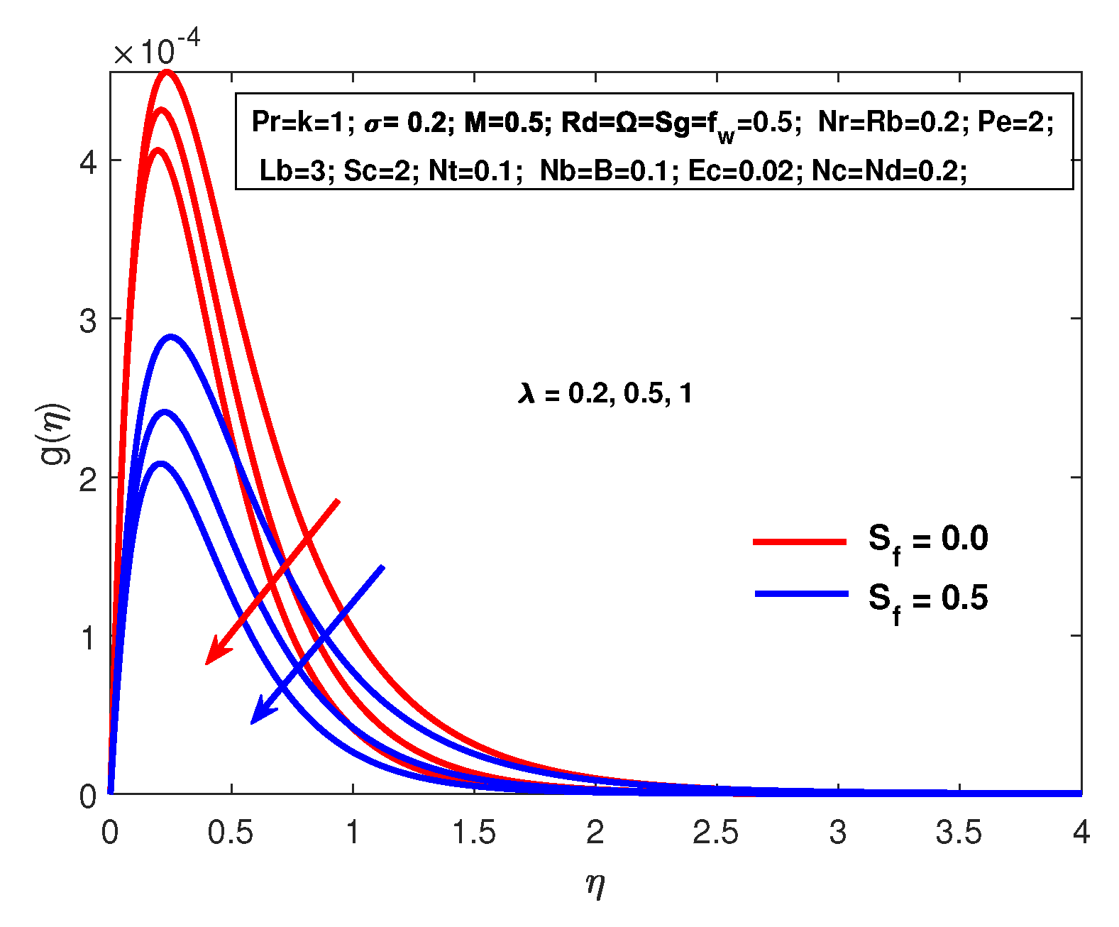
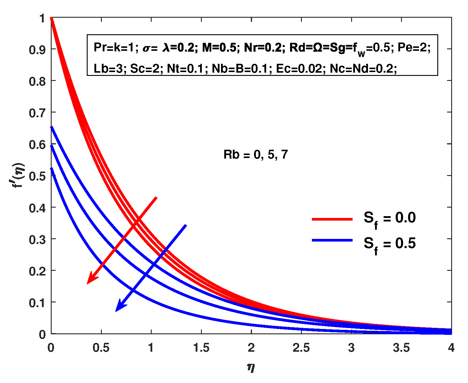
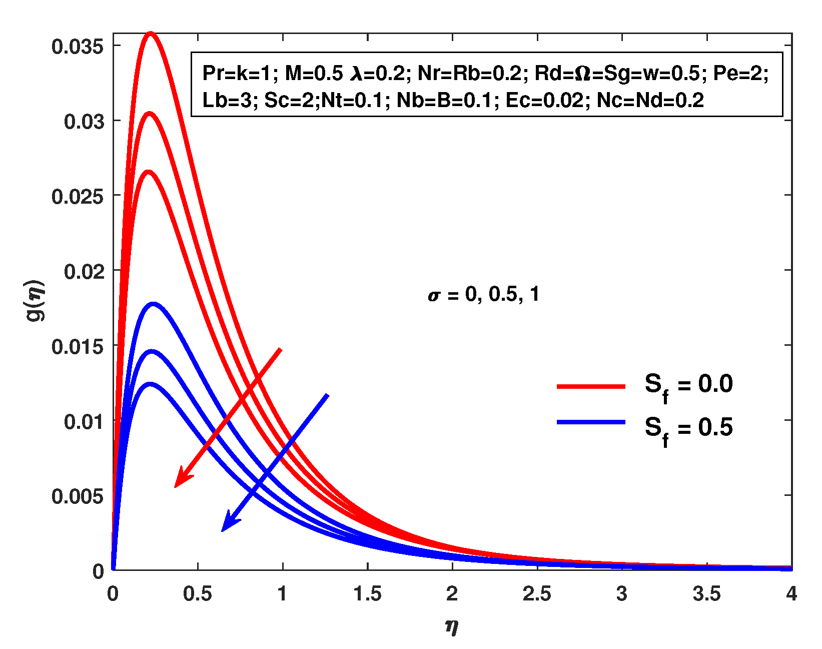
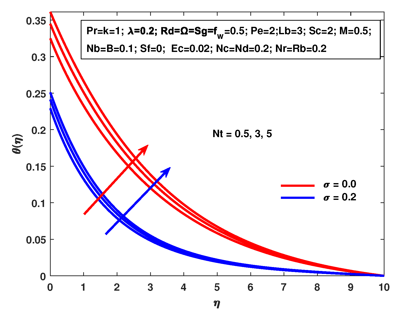
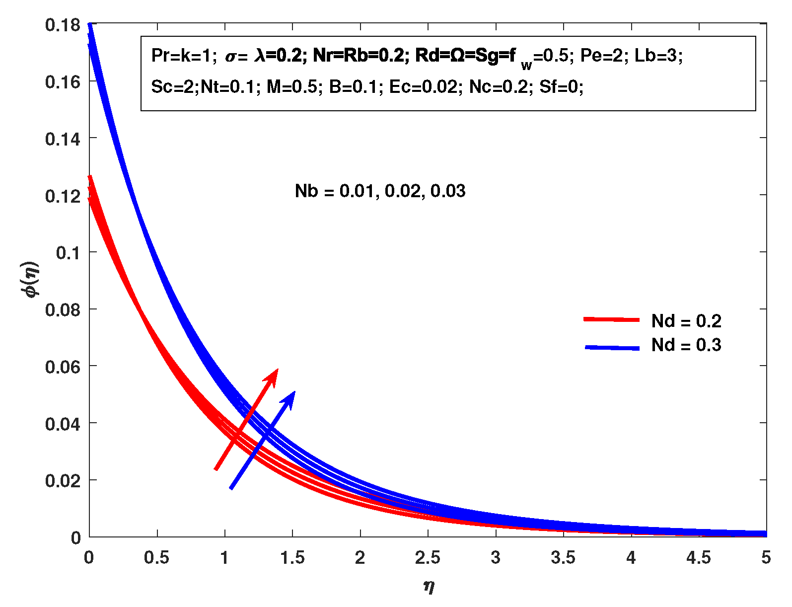
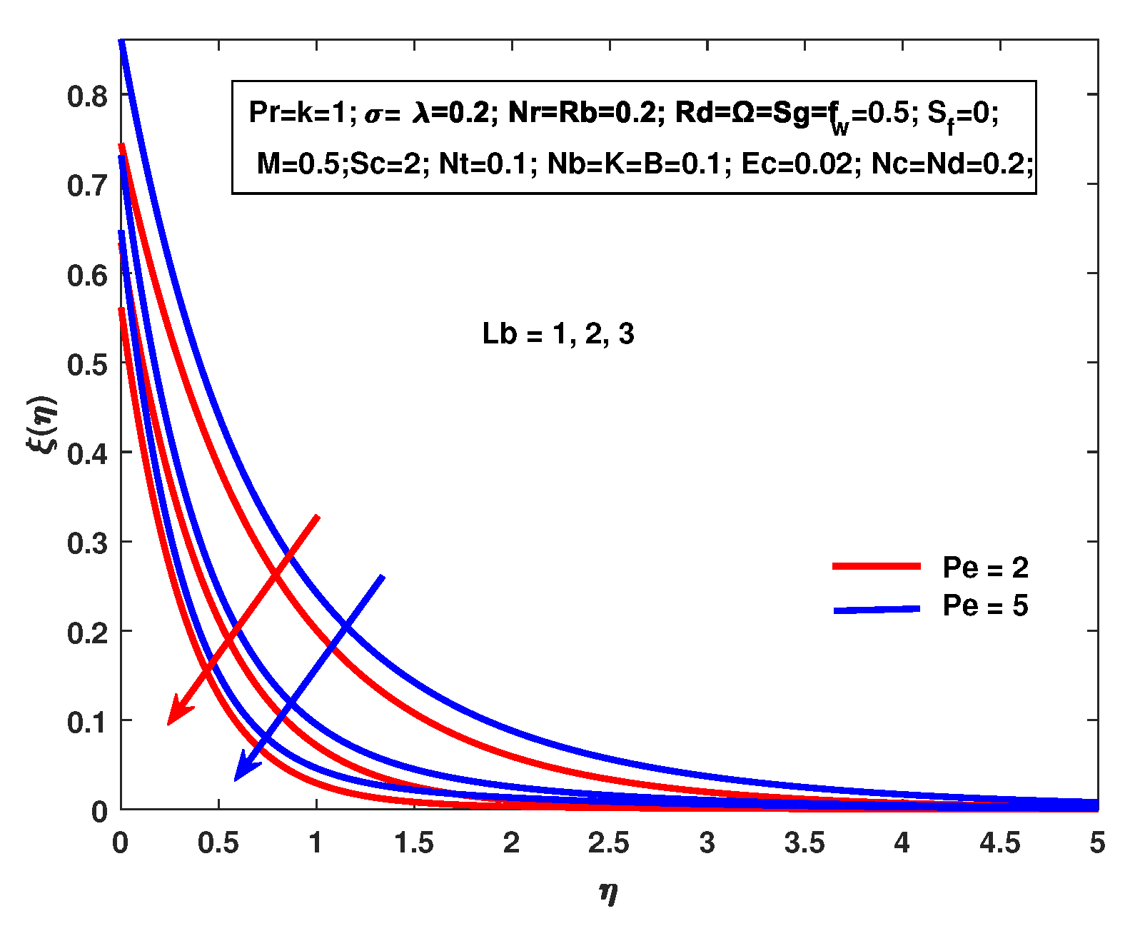
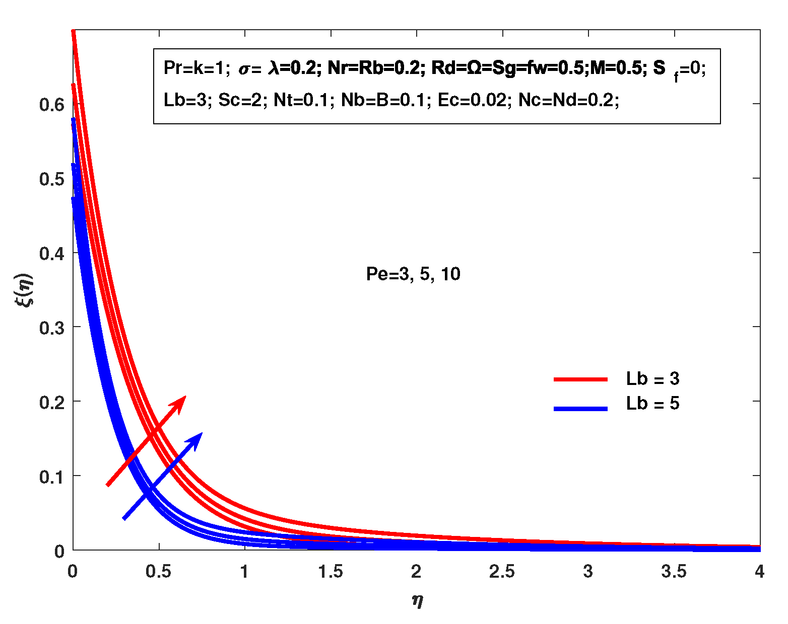
4. Results and Discussion

The numerical computations were executed for the temperature, velocity, solutal and micropolar nanofluid volume fraction functions for a different evaluations of physical parameters, as Prandtl number $Pr$, magnetic parameter M, Unsteadiness $\sigma$, $Nr$ the buoyancy ratio parameter, Brownian motion $Nb$, Rayleigh number $Rb$, thermophoresis $Nt$, Schmidt number $Sc$, $Pe$ Peclet number, $\lambda$ are the buoyancy parameter, $G_r$ the Grashof number, Reynolds number $R_{ex}$, K the micropolar constant, $E_c$ the Eckert number, $L_b$ the bioconvection Lewis parameter, the heat generation coefficient, $R_b$ the Rayleigh numeral, $\mathsf{\Omega }$ the microorganism concentration difference parameter, buoyancy parameter $\lambda$, $f_w$ is Suction/Injection. The detail of the present results and the appraisal of flow velocity is made with the exact solution which consents the validity of the finite element method. It can be seen clearly in

Table 2. Assessment of skin friction coefficient for various values of M and $\sigma$.

M	Mabood and Das	Fazle and Stanford	FEM	$\mathit{\sigma }$	Chamkha et al.	Fazle and Stanford	FEM
	[37]	[34]	(Our Results)		[42]	[34]	(Our Results)
0	−1.000008	−1.0000084	−1.0000082	0.2	–	–	1.068024
1	1.4142135	1.41421356	1.41421353	0.4	–	–	1.134681
5	2.4494897	2.44948974	2.44948963	0.6	–	–	1.199115
10	3.3166247	3.31662479	3.31662463	0.8	1.261512	1.261042	1.261038
50	7.1414284	7.14142843	7.14142839	1.0	–	–	1.320516
100	10.049875	10.0498756	10.0498751	1.2	1.378052	1.377724	1.377718
500	22.383029	22.3830293	22.3830283	1.4	–	–	1.432829
1000	31.638584	31.6385840	31.6385833	1.6	–	–	1.486033

,

Table 3. Assessment of $-{\theta }^{\prime }(0)$ for various values of $Pr$.

$\mathit{Pr}$	Ali [43]	Fazle and Stanford [34]	Ishak et al. [44]	Dulal Pal. [45]	Haile et al. [46]	Ishak et al. [44] (a) Exact Solution	FEM (b) Our Results	Error in % $|(\frac{\mathit{b}-\mathit{a}}{\mathit{a}})|\times 100$
0.72	0.8058	0.8088	–	–	–	0.8086313498	0.8086339302	0.0003
1.00	0.9691	1.0000	1.0000	1.0000	1.0004	1.000000000	1.0000080217	0.0008
3.00	1.9144	1.9237	1.9237	1.9236	1.9234	1.923682594	1.9236777225	0.0003
10.0	3.7006	3.7207	3.7207	3.7207	3.7205	3.720673901	3.7206681690	0.0002
100	–	–	12.2941	12.2940	12.2962	12.294083260	12.294051665	0.0003

and

Table 4. Comparison of $-f^{″}(0)$, and $g^{\prime }(0)$ with recently calculated values when all the other parameters are zero.

M	K	−f″(0)	−f″(0) [48]	Our Results	g′(0)	g′(0) [48]	Our Results
0.0	0.2	0.9098	0.90976	0.909698	0.0950	0.09500	0.094995
0.5	–	1.1148	1.11437	1.114368	0.1051	0.10509	0.105085
1.0	–	1.2871	1.28711	1.287147	0.1121	0.11212	0.112058
–	0.0	1.4142	1.41423	1.414208	0.0000	0.00000	0.000000
–	0.5	1.1408	1.14073	1.140781	0.2112	0.21116	0.211157
–	2.0	0.7697	0.76958	0.769749	0.3586	0.35855	0.358659

. To ensure the accuracy of presented numerical results, the results obtained by finite element method for skin friction co-efficient for the steady and unsteady flow have been compared with the numerical results that have been previously reported in existing studies in Table 2, and regarding our results, there is admirable conformity among our outcomes and previously available research articles that approve the cogency and the accuracy of the current results that are obtained by the finite element method (FEM). Table 2 describes the results of the heat transfer rate that is acquired by the finite element method which is compared with the results of earlier studies and with the accurate solution of references [34,37,42]. We found that our results are in absolute accord and the grid invariance test was executed to sustain accuracy for 5-decimal points.

Table 3 represents the results of the heat transfer rate acquired by FEM that are estimated with the results of earlier studies and the exact result of Ishak et al. [44] in the particular case $(Nt=Nb=0)$. It has been observed that the attained numerical results are in complete accord and a grid invariance test has been performed to preserve four decimal points of correctness.Of all the calculations according to this critique, $\xi (\eta )$ have been elected as ${10}^{-6}$. For more consistency and justifications of the results, the consequences of $-f^{″}(0)$ and $g^{\prime }(0)$ that have been detailed by Hsiao [48] and Eldabe [47] are effectively replicated and shown in Table 4. Figure 2 is evidence for the effect of M on the velocity function with and without hydro-dynamic slip. The results show that in each case the velocity component decreases with increasing value of M. Actually, the magnetic parameter M generated Lorentz force reminiscent of a drag force; that is why there is deceleration of motion of the fluid. Figure 2 also shows that in both conditions the suction $f_w$ deceases the momentum boundary layer thickness that can be controlled with $f_w$.

To observe the consequences of the buoyancy parameter $\lambda$ on the velocity profile with non-existence and the existence of hydrodynamic slip Figure 3 is presented. In this case, we have to perceive that the momentum boundary layer declines with the escalating values of the buoyancy parameter. As to see the effects of the buoyancy ratio parameters on the velocity profile with and without hydro-dynamic slip, as shown in Figure 4. The dimensionless velocity profile $f^{\prime }(\eta )$ is decreasing while the opposite is the case for $Nr$ in the absence of slip and the velocity slip thickness is decreasing with the existence of slip. In Figure 5 it is noted that, due to the disparity in the velocity profile with and without hydro-dynamic slip there is an increase in the bio-convection Rayleigh number $Rb$. In order to increase $Rb$, the buoyancy force is increased, due to which the velocity of the fluid is decelerated. A similar flow prototype was observed by reference [49] in their work.

The impact of $\sigma$ on velocity profile for $S_f=0$ and $S_f=0.5$ is revealed in Figure 6. It is observed that escalating values of $\sigma$ decrease the fluid velocity in the locality of the stretching sheet. Actually, this illustrates that fluid velocity contiguous to the sheet is less than the velocity of the stretching sheet while slither takes place. Escalating $\sigma$ adequately means more fluid slides over the sheet and the flow slump is close to the sheet more rapidly. Furthermore, it shows that the fluid velocity close to the sheet will not remain the same as the sheet stretching velocity as the slide transpire, for that reason; there is indeed velocity. An analogous tendency was inspected by reference [36] in their work. With the increasing values of $Nc$ and $Rd$, Figure 7 illustrates that both the temperature and gyrotactic microorganism concentration increases with an increase in the value of M. The main rationale of this exploit is that temperature and concentration gradients decline as existing transitory through moving fluids and as a result, ascend in thermal and concentration boundary layer thickness. Figure 8 shows the effect of the $Nb$ on temperature $\theta (\eta )$ which reveals that an enrichment in $Nb$ causes an increase in $\theta (\eta )$ at different values of Eckert number $Ec$. A greater thermal boundary layer width is created with high $Nb$ values while higher concentration boundary layer thickness is achieved with lesser $Nb$ values. Both the thermal profile and the associated boundary layer thickness are elevated for the increasing assessments of $Nb$. Figure 9 is shown to envisage the inconsistency in temperature $\theta (\eta )$ due to the thermophoresis parameter $Nt$. Also, it was proved that temperature was enhanced as the thermal boundary layer grows to be thicker for both the steady and unsteady cases.

Figure 10 demonstrates the influence of $Nb$ on $\varphi (\eta )$. The decline in value of $Nb$ is related to an increase in the value of $\varphi (\eta )$. Actually, $Nb$ exacerbates the particles of the fluid regimes; for that reason, an increment is observed in the concentration profile. Figure 11 demonstrates the influence of the magnetic parameter M on $\varphi (\eta )$ for both $Sc=1$ and $Sc=2$. An acclivity in M causes an increase in the value of $\varphi (\eta )$. These curves show an increase in the values of M and enrichment in the concentration profile. Figure 12 shows the motile compactness profile $\xi (\eta )$ for the escalating values of the magnetic numeral M with and without hydro-dynamic slip. These curves revealed that an increase in values of M gives an enrichment in the motile compactness profile $\varphi (\eta )$. The density profile $\xi (\eta )$ is a declining function of Lewis number $Lb$ for $P_e=2$ and $P_e=5$ as exposed in Figure 13. The elevated values of the $Lb$ mean a decrease in the diffusivity of microorganisms, so as a result, $\xi (\eta )$ is reduced.

Figure 14 illustrates the impacts of $Pe$ on the microorganism profile. It illustrates that the microorganism profile is enhanced while escalating the bio-convection Peclet number $Pe$. While $Pe$ contains interrelation by means of maximum cell swimming movement, chemotaxis is constant and the opposite relation in the diffusivity of the microorganism. As a result, for higher values of $Pe$, the microorganisms profile will be enlarged. In Figure 15 it is indomitable that the motile concentration profile $\xi (\eta )$ for unsteady parameter $\sigma$ is enhanced. Furthermore, a decrease in associated boundary layer thicknesses with and without hydro-dynamic slip is also eminent. The discrepancy in motile concentration profile $\xi (\eta )$ due to attachment of assorted parameters and the effect of the material parameter K on the motile concentration profile $\xi (\eta )$, is demonstrated in Figure 16. An enhancement in the value K causes the motile concentration profile $\xi (\eta )$ to decline.

Figure 17 illustrates the impact of M, $Sf$ and $\sigma$ on the skin friction coefficient. It is comprehensible from Figure 17 that the skin friction coefficient declines with the ascending value of the slip parameter, magnetic and unsteadiness parameter and Figure 18 shows the influence of M, $\sigma$ and $S_f$ on $g^{\prime }(0)$. Figure 19 allows the investigation of the effect of M and $\sigma$ on Nusselt number with $S_f=0$ and $f_w=0.5$. It can be observed that the mass transfer ratio enhances as M and $\sigma$ increases. It is also resolute that in the case of nanofluid the mass transfer ratio is larger in disparity by viscous fluid. Lastly, Figure 20 divulged the discrepancy of local Sherwood number for escalating values of magnetic parameter M the bio-convection Lewis parameter $Lb$ and bio-convection Peclet number $Pe$. Intriguingly, the mass transfer rate is seen as an increasing function of $Lb$ and $Pe$. While escalating values of M decreases the mass transfer rate. Thus, it can exemplified that the mass transfer rate decreases as M enhance. All these interpretations are consistent with the consequences that are shown in

Table 5. Different mathematical values of physical constraints M, $\lambda ,Nr,Rb,\sigma ,Pr$ when $Rd=0.5=f_w$, $S_c=8$, $S_f=S_t=S_p=0.3=S_g$, $N_b=N_t=0.1$, $K=0.1$.

M	$\mathit{\lambda }$	$\mathit{Nr}$	$\mathit{Rb}$	$\mathit{\sigma }$	$\mathit{Pr}$	${\mathit{g}}^{\prime }(0)$	$-{\mathit{f}}^{″}(0)$	$-{\mathit{\theta }}^{\prime }(0)$	$-{\mathit{\xi }}^{\prime }(0)$
0.0	0.2	0.2	0.2	0.2	1	0.0273443	0.559615	0.168901	1.417108
0.5	–	–	–	–	–	0.0283705	0.636141	0.167315	1.398302
1.0	–	–	–	–	–	0.0287677	0.695106	0.166101	1.383229
0.5	0.2	0.2	0.2	0.2	1	0.0283702	0.636141	0.167315	1.398302
–	0.4	–	–	–	–	0.0283024	0.632248	0.167371	1.399311
–	0.7	–	–	–	–	0.0282043	0.626489	0.167452	1.400790
0.5	0.2	0.2	0.2	0.2	1	0.0283702	0.636141	0.167315	1.398302
–	–	0.4	–	–	–	0.0283844	0.636741	0.167206	1.398143
–	–	0.7	–	–	–	0.0284058	0.636744	0.167292	1.397903
0.5	0.2	0.2	0.2	0.2	1	0.0283702	0.636141	0.167315	1.398302
–	–	–	0.4	–	–	0.0283531	0.638059	0.167298	1.397888
–	–	–	0.7	–	–	0.0283275	0.640943	0.167273	1.397264
0.5	0.2	0.2	0.2	0.2	1	0.0283702	0.636141	0.167315	1.398302
–	–	–	–	0.6	–	0.0244409	0.673190	0.173017	1.516147
–	–	–	–	1.0	–	0.0220812	0.706038	0.176332	1.609329
0.5	0.2	0.2	0.2	0.2	1	0.0283702	0.636141	0.167315	1.398302
–	–	–	–	–	4	0.0284366	0.641055	0.185297	1.411401
–	–	–	–	–	6	0.0284335	0.641570	0.188534	1.420791

. In Table 5 we analyze the variation of physical parameters M, $\lambda ,N_r,Rb,\sigma ,P_r,L_e$ on skin friction co-efficient velocity $g^{\prime }(0)$, $-f^{″}(0)$, Nusselt number $-{\theta }^{\prime }(0)$, Sherwood number $-{\xi }^{\prime }(0)$.

The following results are concluded from Table 5:

(1)

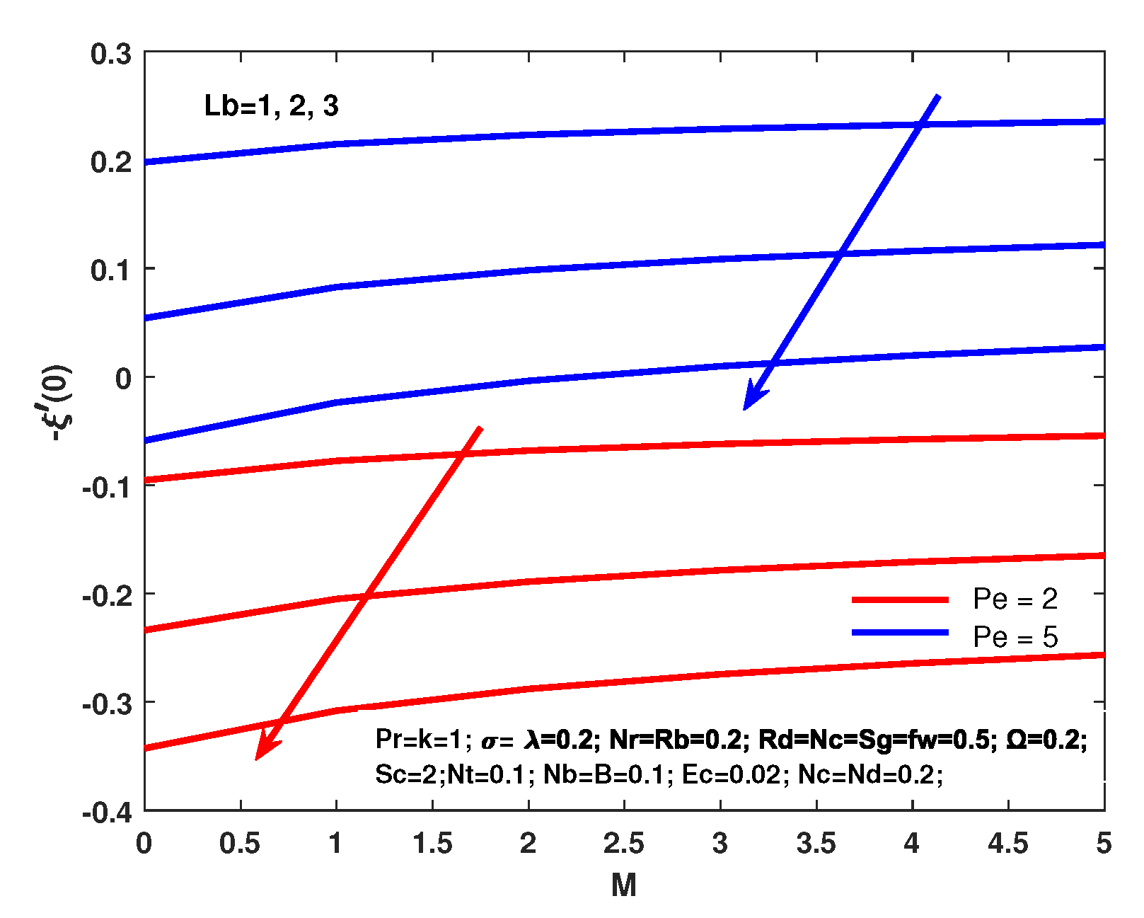
The Skin-friction coefficient and velocity are increasing while reducing the local Nusselt and density number through improvement in the Magnetic parameter.

(2)

The increment in thermal buoyancy parameters $\lambda$, cause decreasing the Skin-friction coefficient and velocity while increasing the local Nusselt number and density number.

(3)

With the increasing unsteadiness parameter $\sigma$ The Skin-friction coefficient, local Nusselt and density numbers are also increasing.

(4)

The Skin-friction coefficient is increasing with the increment in Prandtl number, also increasing the local Nusselt number and velocity.

(5)

The Skin-friction coefficient is increasing with the increasing Rayleigh number and also increment in the local Nusselt number, velocity and density number.

5. Conclusions

An unsteady the flow of magneto-hydrodynamic (MHD) bioconvective micropolar nanofluid containing gyrotactic microorganism has been inspected numerically. The study was performed to analyze the solution of a 2-D laminar bioconvective boundary layer flow of water-based micropolar nanofluids over a stretching sheet. The mathematical sculpt was rehabilitated into the set of coupled ordinary differential equations by applying suitable transformations; the resulting system of ordinary differential equations was evaluated numerically with a proficient and validated finite element method (FEM). FEM is a numerical scheme for the estimation of a parameter-dependent problem that is used to find tht the accuracy of the approximations depreciates as the parameter tends to a limiting value. For the given problem, the present results in Table 3 shows the accuracy, up to four decimal places, of the fast convergence for all values of the parameter. Furthermore, for a particular case, the comparison of the current results with previous studies of the presented model has been discussed. A parametric study has been performed to investigate the influence of various parameters on the velocity, temperature, micro-rotation, gyrotactic microorganism volume fraction and the motile microorganism’s profile. Moreover, local skin friction, heat transfer rate and the motile microorganism’s thickness rate are scrutinized graphically. A few motivating elucidations from the present work are affirmed as,

• The fluid velocity, temperature and gyrotactic microorganism concentration are found to have declined with enhancement in the unsteadiness parameter.
• The Skin-friction coefficient decreases with the increasing value of slip parameters, magnetic and unsteadiness parameter but the effect is the opposite for escalating values of thermal buoyancy, suction parameter and solutal buoyancy.
• The temperature declines, whereas the gyrotactic microorganism concentration decreases with enhancement in values of magnetic parameter M, Brownian motion parameter $Nb$, thermophoresis parameter $Nt$.
• Due to an enhancement in the material parameter K, unsteady parameter as $\sigma$, bio-convection parameter $\lambda$ and bioconvection Lewis parameter $Lb$, the motile concentration profile $\xi (\eta )$ is declined.
• Mass transfer rate increases as Brownian motion parameter $Nb$ increases whereas decreases with enhancement in thermophoresis parameter $Nt$.
• Due to an enhancement in the magnetic parameter M, Peclet number as $Pe$ and bioconvection Lewis parameter $Lb$, the motile concentration profile $\xi (\eta )$ increases.

References

1. Wen, D.; Lin, G.; Vafaei, S.; Zhang, K. Review of nanofluids for heat transfer applications. Particuology 2009, 7, 141–150. [Google Scholar] [CrossRef]
2. Yang, L.; Huang, J.N.; Ji, W.; Mao, M. Investigations of a new combined application of nanofluids in heat recovery and air purification. Powder Technol. 2019. [Google Scholar] [CrossRef]
3. Pradhan, S.; Baag, S.; Mishra, S.; Acharya, M. Free convective MHD micropolar fluid flow with thermal radiation and radiation absorption: A numerical study. Heat Transf. Asian Res. 2019, 48, 2613–2628. [Google Scholar] [CrossRef]
4. Sharada, K.; Shankar, B. MHD mixed convection flow of a Casson fluid over an exponentially stretching surface with the effects of Soret, Dufour, thermal radiation and chemical reaction. World J. Mech. 2015, 5, 165. [Google Scholar] [CrossRef] [Green Version]
5. Moradikazerouni, A.; Afrand, M.; Alsarraf, J.; Mahian, O.; Wongwises, S.; Tran, M.D. Comparison of the effect of five different entrance channel shapes of a micro-channel heat sink in forced convection with application to cooling a supercomputer circuit board. Appl. Therm. Eng. 2019, 150, 1078–1089. [Google Scholar] [CrossRef]
6. Pushpalatha, K.; Reddy, J.R.; Sugunamma, V.; Sandeep, N. Numerical study of chemically reacting unsteady Casson fluid flow past a stretching surface with cross diffusion and thermal radiation. Open Eng. 2017, 7, 69–76. [Google Scholar] [CrossRef]
7. Vo, D.D.; Alsarraf, J.; Moradikazerouni, A.; Afrand, M.; Salehipour, H.; Qi, C. Numerical investigation of γ-AlOOH nanofluid convection performance in a wavy channel considering various shapes of nanoadditives. Powder Technol. 2019, 345, 649–657. [Google Scholar] [CrossRef]
8. Ullah, I.; Nisar, K.S.; Shafie, S.; Khan, I.; Qasim, M.; Khan, A. Unsteady free convection flow of casson nanofluid over a nonlinear stretching sheet. IEEE Access 2019, 7, 93076–93087. [Google Scholar] [CrossRef]
9. Uddin, M.J.; Khan, W.; Ismail, A.M. Free convection boundary layer flow from a heated upward facing horizontal flat plate embedded in a porous medium filled by a nanofluid with convective boundary condition. Transp. Porous Media 2012, 92, 867–881. [Google Scholar] [CrossRef]
10. Alsarraf, J.; Moradikazerouni, A.; Shahsavar, A.; Afrand, M.; Salehipour, H.; Tran, M.D. Hydrothermal analysis of turbulent boehmite alumina nanofluid flow with different nanoparticle shapes in a minichannel heat exchanger using two-phase mixture model. Phys. A Stat. Mech. Appl. 2019, 520, 275–288. [Google Scholar] [CrossRef]
11. Moradikazerouni, A.; Afrand, M.; Alsarraf, J.; Wongwises, S.; Asadi, A.; Nguyen, T.K. Investigation of a computer CPU heat sink under laminar forced convection using a structural stability method. Int. J. Heat Mass Transf. 2019, 134, 1218–1226. [Google Scholar] [CrossRef]
12. Ranjbarzadeh, R.; Moradikazerouni, A.; Bakhtiari, R.; Asadi, A.; Afrand, M. An experimental study on stability and thermal conductivity of water/silica nanofluid: Eco-friendly production of nanoparticles. J. Clean. Prod. 2019, 206, 1089–1100. [Google Scholar] [CrossRef]
13. Naseem, F.; Shafiq, A.; Zhao, L.; Naseem, A. MHD biconvective flow of Powell Eyringnanofluid over stretched surface. AIP Adv. 2017, 7, 065013. [Google Scholar] [CrossRef] [Green Version]
14. Lee, T.; Parikh, P.; Acrivos, A.; Bershader, D. Natural convection in a vertical channel with opposing buoyancy forces. Int. J. Heat Mass Transf. 1982, 25, 499–511. [Google Scholar] [CrossRef]
15. Das, K.; Duari, P.; Kundu, P.K. Nanofluidbioconvection in presence of gyrotactic microorganisms and chemical reaction in a porous medium. J. Mech. Sci. Technol. 2015, 29, 4841–4849. [Google Scholar] [CrossRef]
16. Khan, U.; Ahmed, N.; Mohyud-Din, S.T. Influence of viscous dissipation and Joule heating on MHD bio-convection flow over a porous wedge in the presence of nanoparticles and gyrotactic microorganisms. SpringerPlus 2016, 5, 2043. [Google Scholar] [CrossRef] [Green Version]
17. Kuznetsov, A.V. Nanofluidbioconvection in porous media: oxytactic microorganisms. J. Porous Media 2012, 15, 233–248. [Google Scholar] [CrossRef]
18. Khan, W.; Makinde, O.; Khan, Z. MHD boundary layer flow of a nanofluid containing gyrotactic microorganisms past a vertical plate with Navier slip. Int. J. Heat Mass Transf. 2014, 74, 285–291. [Google Scholar] [CrossRef]
19. Rahman, M.; Al-Lawatia, M.; Eltayeb, I.; Al-Salti, N. Hydromagnetic slip flow of water based nanofluids past a wedge with convective surface in the presence of heat generation (or) absorption. Int. J. Therm. Sci. 2012, 57, 172–182. [Google Scholar] [CrossRef]
20. Ibrahim, W.; Shankar, B. MHD boundary layer flow and heat transfer of a nanofluid past a permeable stretching sheet with velocity, thermal and solutal slip boundary conditions. Comput. Fluids 2013, 75, 1–10. [Google Scholar] [CrossRef]
21. Ma, Y.; Shahsavar, A.; Moradi, I.; Rostami, S.; Moradikazerouni, A.; Yarmand, H.; Zulkifli, N.W.B.M. Using finite volume method for simulating the natural convective heat transfer of nanofluid flow inside an inclined enclosure with conductive walls in the presence of a constant temperature heat source. Phys. A Stat. Mech. Appl. 2019. [Google Scholar] [CrossRef]
22. Das, K. Slip flow and convective heat transfer of nanofluids over a permeable stretching surface. Comput. Fluids 2012, 64, 34–42. [Google Scholar] [CrossRef]
23. Abbas, Z.; Wang, Y.; Hayat, T.; Oberlack, M. Slip effects and heat transfer analysis in a viscous fluid over an oscillatory stretching surface. Int. J. Numer. Methods Fluids 2009, 59, 443–458. [Google Scholar] [CrossRef]
24. Makinde, O.D.; Mabood, F.; Ibrahim, M.S. Chemically reacting on MHD boundary-layer flow of nanofluids over a non-linear stretching sheet with heat source/sink and thermal radiation. Therm. Sci. 2018, 22, 495–506. [Google Scholar] [CrossRef]
25. Aziz, A.; Khan, W.; Pop, I. Free convection boundary layer flow past a horizontal flat plate embedded in porous medium filled by nanofluid containing gyrotactic microorganisms. Int. J. Therm. Sci. 2012, 56, 48–57. [Google Scholar] [CrossRef]
26. Buongiorno, J. Convective transport in nanofluids. J. Heat Transf. 2006, 128, 240–250. [Google Scholar] [CrossRef]
27. Pit, R.; Hervet, H.; Leger, L. Direct experimental evidence of slip in hexadecane: Solid interfaces. Phys. Rev. Lett. 2000, 85, 980. [Google Scholar] [CrossRef]
28. Wu, X.; Wu, H.; Cheng, P. Pressure drop and heat transfer of Al2O3-H2O nanofluids through silicon microchannels. J. Micromech. Microeng. 2009, 19, 105020. [Google Scholar] [CrossRef]
29. Xu, H.; Pop, I. Fully developed mixed convection flow in a horizontal channel filled by a nanofluid containing both nanoparticles and gyrotactic microorganisms. Eur. J. Mech. B/Fluids 2014, 46, 37–45. [Google Scholar] [CrossRef]
30. Siddiqa, S.; Begum, N.; Saleem, S.; Hossain, M.A.; Gorla, R.S.R. Numerical solutions of nanofluid bioconvection due to gyrotactic microorganisms along a vertical wavy cone. Int. J. Heat Mass Transf. 2016, 101, 608–613. [Google Scholar] [CrossRef]
31. Bin-Mohsin, B.; Ahmed, N.; Khan, U.; Mohyud-Din, S.T. A bioconvection model for a squeezing flow of nanofluid between parallel plates in the presence of gyrotactic microorganisms. Eur. Phys. J. Plus 2017, 132, 187. [Google Scholar] [CrossRef]
32. Li, Z.; Sheikholeslami, M.; Chamkha, A.J.; Raizah, Z.; Saleem, S. Control volume finite element method for nanofluid MHD natural convective flow inside a sinusoidal annulus under the impact of thermal radiation. Comput. Methods Appl. Mech. Eng. 2018, 338, 618–633. [Google Scholar] [CrossRef]
33. Mahian, O.; Kolsi, L.; Amani, M.; Estellé, P.; Ahmadi, G.; Kleinstreuer, C.; Marshall, J.S.; Siavashi, M.; Taylor, R.A.; Niazmand, H.; et al. Recent advances in modeling and simulation of nanofluid flows—Part I: Fundamental and theory. Phys. Rep. 2018, 790, 1–48. [Google Scholar] [CrossRef]
34. Mabood, F.; Shateyi, S. Multiple slip effects on MHD unsteady flow heat and mass transfer impinging on permeable stretching sheet with radiation. Model. Simul. Eng. 2019, 2019, 3052790. [Google Scholar] [CrossRef] [Green Version]
35. Malarselvi, A.; Bhuvaneswari, M.; Sivasankaran, S.; Ganga, B.; Hakeem, A.A. Effect of slip and convective heating on unsteady MHD chemically reacting flow over a porous surface with suction. In Applied Mathematics and Scientific Computing; Springer: Berlin/Heidelberg, Germany, 2019; pp. 357–365. [Google Scholar]
36. Ali, B.; Nie, Y.; Khan, S.A.; Sadiq, M.T.; Tariq, M. Finite element simulation of multiple slip effects on MHD unsteady maxwell nanofluid flow over a permeable stretching sheet with radiation and thermo-diffusion in the presence of chemical reaction. Processes 2019, 7, 628. [Google Scholar] [CrossRef] [Green Version]
37. Mabood, F.; Das, K. Melting heat transfer on hydromagnetic flow of a nanofluid over a stretching sheet with radiation and second-order slip. Eur. Phys. J. Plus 2016, 131, 3. [Google Scholar] [CrossRef]
38. Reddy, J.N. An Introduction to the Finite Element Method; McGraw-Hill Education: New York, NY, USA, 1993. [Google Scholar]
39. Swapna, G.; Kumar, L.; Rana, P.; Singh, B. Finite element modeling of a double-diffusive mixed convection flow of a chemically-reacting magneto-micropolar fluid with convective boundary condition. J. Taiwan Inst. Chem. Eng. 2015, 47, 18–27. [Google Scholar] [CrossRef]
40. Gupta, D.; Kumar, L.; Beg, O.A.; Singh, B. Finite-element analysis of transient heat and mass transfer in microstructural boundary layer flow from a porous stretching sheet. Comput. Therm. Sci. Int. J. 2014, 6, 155–169. [Google Scholar] [CrossRef]
41. Uddin, M.; Rana, P.; Bég, O.A.; Ismail, A.M. Finite element simulation of magnetohydrodynamic convective nanofluid slip flow in porous media with nonlinear radiation. Alex. Eng. J. 2016, 55, 1305–1319. [Google Scholar] [CrossRef]
42. Chamkha, A.; Aly, A.; Mansour, M. Similarity solution for unsteady heat and mass transfer from a stretching surface embedded in a porous medium with suction/injection and chemical reaction effects. Chem. Eng. Commun. 2010, 197, 846–858. [Google Scholar] [CrossRef]
43. Ali, M.E. Heat transfer characteristics of a continuous stretching surface. Wärme-und Stoffübertragung 1994, 29, 227–234. [Google Scholar] [CrossRef]
44. Ishak, A.; Nazar, R.; Pop, I. Boundary layer flow and heat transfer over an unsteady stretching vertical surface. Meccanica 2009, 44, 369–375. [Google Scholar] [CrossRef]
45. Pal, D. Combined effects of non-uniform heat source/sink and thermal radiation on heat transfer over an unsteady stretching permeable surface. Commun. Nonlinear Sci. Numer. Simul. 2011, 16, 1890–1904. [Google Scholar] [CrossRef]
46. Haile, E.; Shankar, B. Heat and mass transfer in the boundary layer of unsteady viscous nanofluid along a vertical stretching sheet. J. Comput. Eng. 2014, 2014, 345153. [Google Scholar] [CrossRef] [Green Version]
47. Eldabe, N.T.; Ouaf, M.E. Chebyshev finite difference method for heat and mass transfer in a hydromagnetic flow of a micropolar fluid past a stretching surface with Ohmic heating and viscous dissipation. Appl. Math. Comput. 2006, 177, 561–571. [Google Scholar] [CrossRef]
48. Hsiao, K.L. Micropolar nanofluid flow with MHD and viscous dissipation effects towards a stretching sheet with multimedia feature. Int. J. Heat Mass Transf. 2017, 112, 983–990. [Google Scholar] [CrossRef]
49. Atif, S.; Hussain, S.; Sagheer, M. Magnetohydrodynamic stratified bioconvective flow of micropolar nanofluid due to gyrotactic microorganisms. AIP Adv. 2019, 9, 025208. [Google Scholar] [CrossRef] [Green Version]
Figure 1. Physically sketch with x y -coordinates.
Coatings 09 00842 g001
Figure 2. Effects of M and S f on f .
Coatings 09 00842 g002
Figure 3. Effects of λ and S f on g.
Coatings 09 00842 g003
Figure 4. Effects of N r and S f on f .
Coatings 09 00842 g004
Figure 5. Effects of R b , and S f on f .
Coatings 09 00842 g005
Figure 6. Effects of σ and S f on g.
Coatings 09 00842 g006
Figure 7. Effects of M, N c and R d on θ .
Coatings 09 00842 g007
Figure 8. Effects of N b and E c on θ .
Coatings 09 00842 g008
Figure 9. Effects of N t and σ on θ .
Coatings 09 00842 g009
Figure 10. Effects of N b and N d on ϕ .
Coatings 09 00842 g010
Figure 11. Effects of M and S c on ϕ .
Coatings 09 00842 g011
Figure 12. Effects of M and S g on ξ .
Coatings 09 00842 g012
Figure 13. Effects of L b and P e on ξ .
Coatings 09 00842 g013
Figure 14. Effects of P e and L b on ξ .
Coatings 09 00842 g014
Figure 15. Effects of σ and S g on ξ .
Coatings 09 00842 g015
Figure 16. Effects of K and f w on ξ .
Coatings 09 00842 g016
Figure 17. Effect of different values of M, σ and S f on Skin friction number.
Coatings 09 00842 g017
Figure 18. Effect of different values of M, σ and S f on g ( 0 ) .
Coatings 09 00842 g018
Figure 19. Effect of different values of M, σ and S f on reduced Nusselt number.
Coatings 09 00842 g019
Figure 20. Effect of different values of M, L b and P e on reduced Microorganism number.
Coatings 09 00842 g020