Article

Dynamic Optimization of Fuel and Logistics Costs as a Tool in Pursuing Economic Sustainability of a Farm

1
School of Economics and Management, Harbin Engineering University, Harbin 150001, China
2
Faculty of Economics, RUDN University, Moscow 117198, Russia
*
Author to whom correspondence should be addressed.
Sustainability 2019, 11(19), 5463; https://doi.org/10.3390/su11195463
Submission received: 26 August 2019 / Revised: 29 September 2019 / Accepted: 30 September 2019 / Published: 2 October 2019

Abstract

:
Improving the performance and economic sustainability of agricultural producers requires the integration of many dimensions, one of which is logistics. Establishing efficient and cost-effective transportation is a key element of establishing sustainable linkages along food supply chains between farmers, storage and transport companies, and consumers. In this regard, infrastructural constraints to sustainability in agricultural production exacerbate transportation costs and risks, and thus result in lower performance of agricultural producers. As fuel consumption is, first, the most significant cost in agricultural logistics and, second, particularly sensitive to disruptions of transport, loading, and storage infrastructure, management of fuel costs is crucial to assure profit margin of an agricultural enterprise. By transforming the standard economic order quantity (EOQ) model, the authors attempt to build an approach to the optimization of fuel costs. The analysis made in the cases of twelve large crop farms in three territories of Southern Russia allowed the consideration of: (1) fragmentation in storage infrastructure; (2) variations in fuel consumption depending on the vehicle load ratio; (3) the use of their own fleet of vehicles against the outsourcing of transport operations. The authors find that the tactics of optimization of fuel costs vary depending on the location of a farm in relation to grain storage facilities. Particularly, the farms located in areas of high concentration of storage facilities benefit from using their own fleet of vehicles, while those experiencing longer distances of transportation should outsource the performance of logistics operations to third parties. To overcome a site-specific nature, the transformed EOQ model should accommodate country-specific requirements, specifically, the level of fragmentation of transport and storage infrastructure, average distance of transportation from a farm to receival site, and average fuel consumption rates depending on the types of trucks commonly used by farmers. The key recommendation is that sustainability-aimed management of logistics costs should consider combining the operation of trucks by a farm with the outsourcing of transportation operations to address the fragmentation of transport and storage infrastructure.

1. Introduction

Logistics costs often represent a large portion of total supply chain costs [1], which is why cost reduction has always been one of the major performance objectives in logistics management [2,3,4]. Total logistic costs reveal much about the locational dynamics of logistics activities, particularly distribution centers, since they indicate the weight of the most important factors [5].
The methods for determining logistics costs vary depending on many parameters, including the type of industry, main components of logistics activities, and cost-accounting or macro context [6,7]. There have been several levels suggested on which the components of logistics costs can be broken down. Sople [8] identified three cost components, transportation, storage, and inventories, while Rushton et al. [9] added administration costs to those three. Ayers [10] identified five components of logistics costs: purchased materials and the associated labor, transportation, warehousing, inventories, and packaging. Lambert et al. [11] and Zeng and Rossetti [12] ended up with another set of five key logistics cost elements: transportation, warehousing, order processing/customer service, administration, and inventory holding.
One of the most common ways to systemize logistics costs is to place them along the dimensions of direct, indirect, overhead, and function-related costs (Table 1).
In the majority of the studies, transportation costs remained the dominant consideration, as they account for about half of the logistic costs internationally [14]. In common costing terminology in transport, direct costs are those directly attributed to a vehicle (fuel, insurance, road license), while indirect ones are general costs that result from running a business, referred to as overhead, administrative, or establishment costs, and are spread equally amongst the vehicles in use [9]. Alongside this common breakout, transport costs are broken down into three types: standing, running, and overhead (the first two classified as direct costs, the latter one borne by the whole fleet of vehicles) (Table 2).
Transportation has one of the most critical impacts on the performance efficiency of an organization [15], since the availability of road infrastructure and transport services increases mobility and encourages production [16]. El Bouzekri et al. [17] recognized transportation as an irreplaceable part of the supply chain, through which economic development was possible. Rantasila and Ojala [13] and Gonzalez et al. [18] also identified transportation costs as one of the major drivers affecting the competitiveness of a firm. While the development of transport systems affects production and logistics in a positive way, it also introduces additional challenges to many sectors because it increases the load on transport networks, reliability problems, and the capacity of existing transport infrastructure to accommodate higher flow rates and translate them to the reduced per unit costs. The management of logistics costs is particularly relevant in agriculture, where distribution infrastructure is not well developed and often partial [19]. High logistics cost is one of the major factors that hinders agricultural producers, particularly small and medium ones, from being competitive in the market [20]. Bosona [21] indicated that transportation and other costs, such as inventory, warehousing, and administration costs, could significantly constrain the competitiveness of food producers. In rural areas, high transportation costs and risks are exacerbated by poor local level roads and inefficient transport infrastructure network and services, which, taken together, result in a low level of coordination between agricultural producers and market failures [22].
The cost of fuel is normally the largest of all the transportation costs [9,23]. Fuel is a particularly significant cost in agriculture due to two major reasons. First, the fuel consumption of specialized agricultural machinery and transport vehicles is higher compared to average commercial vehicles. Second, agricultural enterprises have to establish and keep substantial reserves of fuel during winter due to seasonality in agricultural activities. Third, fuel costs are more vulnerable compared to other types of costs because of the constant rise in energy costs due to the shortages in the season of high demand (spring–autumn) [24]. Reduction of fuel costs contributes the most to the increase in the profit margin of agricultural enterprises [25], reduction of per unit costs of commodities with high fixed costs [26], enlargement of the market areas [27], and thus allows for a larger number of agricultural producers to specialize and localize. The concentration of farms, food industries, and wholesalers into a smaller number with large sizes is the main characteristic describing the current trend in the agricultural sector in many countries [21,28]. Even in land-abundant countries, large farms are emerging, in part, as a response to the market and infrastructural, including logistics, deficiencies faced by agricultural producers [29]. For instance, in Russia, the concentration of agricultural producers and greater specialization in output across districts have been common features of agricultural recovery during the 2000–2010s [30]. There are 76,000 growers in Russia producing over 107 mmt of crops annually, but the majority of them are in the southern and central parts of the country. Large-scale farms account for 75% of production [31]. Over recent years, Russia has restructured its key infrastructural bottlenecks, but still experiences logistics problems [32]. On-farm storage capacity is only 45–50% of an average harvest. Crop producers, therefore, use off-farm storage facilities, many of which are outdated, of low storage capacity, and unevenly distributed across the country. Logistics costs thus escalate due to the long distances of transportation and underdeveloped transport and storage infrastructure. Both size and vertical integration help agricultural producers to respond to market and infrastructural imperfections [33], but in the situation of fragmented distribution, the share of the transportation cost per unit of the product have increased.
The management of fuel costs in food supply chains has received more and more attention due to many reasons, including increasing transportation between production facilities, the roles and the types of operations performed in facilities, capacities allocated to each facility, markets that facilities will serve and sources that will feed facilities [34], traceability of food quality and the potential market for local food producers [35], and the increasing consumption of fuel and the associated environmental impact [21]. There is, however, a major challenge most frequently mentioned in the results of the existing studies in the field of fuel costs management in agriculture: the research methods are not unified are fuel cost components are not sufficiently standardized, thus the results are not comparable. Additional challenges include difficulties related to collecting transparent information about the complexity of logistics activities and calculating the costs with due account to a variety of fuel consumption rates of different types of machinery involved in the transportation. The existing methodologies for evaluating logistics costs in agriculture are sparse due to the variety of cost items involved and the complexity of relationships within the logistics system. As more agricultural organizations are outsourcing their transportation activities to specialized companies, it becomes increasingly critical to understand and evaluate logistics costs associated with transportation and fuel in order to assure the profit margin. In view of the lack of inventory in previously conducted studies on logistics costs in agriculture, the purpose of this paper is to develop a reliable method of optimization of total logistics costs by means of fuel costs and thus provide an approach for evaluating and monitoring the logistics performance of an agricultural organization and establish its economic sustainability.

2. Materials and Methods

In the optimization of fuel costs, the variability of the fuel–logistics costs model is preconditioned by three factors: (1) the volatility of fuel prices; (2) dynamic changes in the cost of logistics outsourcing (transportation from supplier to agricultural enterprise); (3) fuel consumption by agricultural enterprises in different stages of the production cycle [36]. In many studies, the complexity of interrelations between the dynamic factors has been addressed by the adoption of the economic order quantity (EOQ) model for the assessment of fuel and logistics costs. One of the first attempts to consider a tradeoff between fixed ordering cost and inventory carrying cost was made by Harris [37], whose deterministic inventory planning model laid the foundation for various kinds of extensions of mathematical modeling to guide managers in making business decisions [38]. Harris’ model was further generalized by Wilson [39], who derived the formula to obtain the economic order quantity. The standard EOQ model assumes that demand is constant, and that inventory is depleted at a fixed rate until it reaches zero [40] (Equation (1)):
V   =   2 × C c × C f C s ,
where V = volume of fuel required for continuing operation of a farm, L; Cc = consignment cost/fuel, $; Cf = fuel consumption of a farm, L; Cs = storage cost/fuel, $.
The model is considered an appropriate tool for calculating the reorder point and the optimal reorder quantity to ensure the instantaneous replenishment of inventory with no shortages [40]. Khan et al. [41], Rao and Bahari-Kashani [42], Huang et al. [43], and Pentico and Drake [44] regarded the EOQ model as a valuable tool for managers who make decisions about how much inventory to keep on hand to incur the lowest possible costs.
Based on the initial assumptions made by Harris [37], further research on the EOQ has evolved in three major directions: logistics, lot-sizing rules, and extensions.
Substantiating the application of the EOQ model in transportation and logistics, Ghasemi and Nadjafi [45] determined the optimum total costs, economic ordering quantity, and related optimum quantity to the ordering cycle length. Keskin et al. [46] used the EOQ model to optimize total logistics costs, including transportation, inventory replenishment, and storage costs. In agricultural logistics, employment of the model allows a decision to be made on the gross volume of fuel Cf required for continuing agricultural production and operation of a farm (Equation (2)):
C f   =   D × F C R 100 × N × T ,
where Cf = fuel consumption in a farm, L; D = total distance per vehicle, km; FCR = fuel consumption rate, L per 100 km; N = cargo vehicles operated by a farm during a year, number of vehicles; T = trips per vehicle, number of trips.
A series of studies investigated the performance of the EOQ model against the quantity of an item ordered for delivery, or lot size. Evan [47] was among the first who demonstrated a significant relationship between lot size and the quality of a product, while Melnyk and Piper [48] examined the effects of lead time errors on logistics performance and efficiency.
The variety of extensions of the EOQ model includes, among others, the development of cost elements of the standard EOQ model by detaching the capital cost as a determinant factor [49], application to retail cycle stock inventories [50], inclusion of storage size considerations [42], and the integration of product pricing and order sizing decisions [51]. A number of studies have explored the extension of the EOQ model in agriculture. Commonly, in agricultural logistics, the rationale of employing the EOQ model is that it provides a good indication of whether or not the parameters of the agricultural logistics chain are reasonable, even if varied dynamic factors do not hold exactly. Hu et al. [52] complemented the EOQ model by multiple cycles’ theory to address decreasing characteristics of agricultural products. Arskiy [36,53] explored the efficiency of the use of the EOQ model in logistical costs calculations in small farms. Chen et al. [54] provided a method to determine the optimal replenishment policy of integrated agricultural supply chains with stochastic demand based on the EOQ and EPQ (Economic Production Quantity) models. Most of the studies above, however, resulted in a finding that the use of the standard model in multiunit and multimodal supply chains encountered challenges and difficulties. Since the standard EOQ model deals with gross consumption of fuel per particular distance of transportation, it thus does not allow the consideration of the variations between the modes of transportation (loaded or empty trip) or the modes of storage (trips between enterprise’s storage facilities, outsourcer’s warehouse, fuel and grain hubs). Depending on who executes the storage, Cs may be calculated in different ways. In the case of an agricultural organization storing the fuel on its premises, Cs is the maintenance cost, which includes the operation and repair of fuel tanks, depreciation charges, property tax, insurance premium, electricity, and water. In a case where the storage is outsourced, Cs simplifies to the cost of the warehouse lease or custody contract [53]. Similar to Cs, consignment cost Cc is determined in various manners depending on the organization which performs transportation. When performed by an agricultural organization itself, the delivery of the agricultural product or fuel is associated with the cost of operation and maintenance of trucks, their depreciation, cost of fuel consumed during transportation, transport tax, and insurance, among other expenditures. When delivery is outsourced, Cc is a price an agricultural organization pays to its contractor [55].
Irrespective of the particular mode of storage and delivery, fuel consumption rate is a major parameter which affects both storage and consignment costs [56]. Notably, despite the clear practical importance of the influence of fuel consumption on management decisions in agricultural logistics, this parameter has been rarely adopted by the EOQ models in the previous literature. Therefore, the authors seek to bridge this gap by finding an appropriate value of Cf crucial for the optimization of logistics costs of both the storage of a particular volume (required marginal reserve) of fuel and cost efficiency of available financial resources. Chen et al. [54] and Tebekin [57] reported the implementation of the EOQ model as promising in large agricultural enterprises where logistics planning was based on the system analysis of external and internal environments and the application of corrections in accordance with the influence of dynamic factors. Accordingly, this study involved twelve large agricultural enterprises located in three territories of Southern Russia, namely, Stavropol, Krasnodar, and Rostov. Rada et al. [30] reported the southern district of Russia as the leading region of Russia’s agricultural revival, where producers appeared to have exploited climatic, infrastructural, and institutional comparative advantages over other districts. The rationale of the choice is that, first, southern parts of Russia are the major producers of agricultural commodities (the three regions taken together provide 16.6% of the gross domestic agricultural production of the country, including 22.0% of the overall national production of crops [58]), second, the agricultural sector is dominated by large enterprises (over 20,000 hectares in size), many of which descended from giant ex-Soviet collective farms [59]. The study included agricultural enterprises specialized in crop production, particularly winter wheat, sunflower, and corn as major crops produced in the South of Russia. The rationale of focusing on crop farms is that they do not commonly establish their own storage facilities to keep agricultural crops but use large grain elevators instead. In the meantime, in the South of Russia, agricultural logistics infrastructure is underdeveloped and fragmented, many of the grain storage facilities are outdated and of low capacity. Therefore, large crop farms are bound to use transportation intensively to maintain regular traffic between fields, temporary storage facilities, grain elevators, and distribution hubs.
To reflect the country-specific fragmentation of transport and storage infrastructure, in this study, the standard EOQ model accommodated the following transformations:
Transformation 1. Many authors, including Saha et al. [60], Lin and Chung [61], and Gerami and Shidlovskiy [62], formulated the EOQ model by considering two facilities (particularly warehouses): the one owned by the organization and the other one rented. Eksler et al. [63] introduced a dependency factor to reflect a correlation between two products transported, stored, and distributed by a firm simultaneously. Drezner et al. [64] presented the model with two substitute products and found that only partial substitution or no substitution might be optimal due to the non-linearity of the decision variables in the total cost expression. Differentiation between delivery points, however, has been less considered. The authors’ transformation of the standard EOQ model thus accommodated the differentiation between transportation to/from farm’s field storage facilities and/or outside warehouse, contractor’s storage, and intermediate fuel or grain hubs to reflect the variations in the distribution of costs depending on who performs storage and transportation.
Transformation 2. Few extensions of the standard model have addressed a differentiation between loaded and empty trips. Ben-Chaim et al. [65] proposed a model in which vehicle fuel consumption was separated into cruising at constant speed and acceleration, but did not take into account fuel consumption during idle mode. Ramirez et al. [66] analyzed fuel consumption behavior with several options of performance metrics, including gross weight of transportation and empty vehicle weight, but did not validate the variability of loads. To reflect the variations in fuel consumption depending on the vehicle load ratio, the authors’ variant of the model estimated differentiations between (1) distances between the farm, receival site, and fuel distribution point and (2) fuel consumption rates in loaded and empty trips (Equation (3)):
C f   =   ( D 1 × F C R l 100 + D 2 × F C R e 100 ) × N × T + R ,
where Cf = fuel consumption in a farm, L; D1 = distance between farm and receival site, km; D2 = distance between receival site, fuel distribution point, and farm, km; FCRl = fuel consumption rate/loaded trip, L per 100 km; FCRe = fuel consumption rate/empty trip, L per 100 km; N = cargo vehicles operated by a farm during a year, number of vehicles; T = trips per vehicle, number of trips; R = fuel reserve, L.
Transformation 3. In earlier studies, Zoldy and Zsombok [67], Nkakini et al. [68], Zhou and Jin [69], and Huertas et al. [70] attempted to incorporate various external and internal parameters, including vehicle driven, road related, usage related, and ambient parameters, that could have predictive effect on fuel consumption and refueling of the vehicle. To the best of the authors’ knowledge, none of the studies have employed the EOQ model to measure the variations in fuel consumption, while the models which were used in the abovementioned studies cannot provide satisfactory predictions for vehicles operating under the conditions of underdeveloped and disrupted logistics chains. To respond to irregular logistics risks (fuel overrun, increase in consumption rate due to heavy road traffic, etc.), the authors complemented the standard EOQ model with fuel reserve provisioning.
Standard (Equation (4)) and transformed (Equation (5)) models were applied consecutively to agricultural enterprises under study to reveal the deviation of the actual volume of fuel reserve maintained in 2013–2017 (Vs) from the optimal one (Vt):
V s   =   2 × C c × D × F C R 100 × N × T C s ,
where Vs = volume of fuel required for continuous operation of a farm/standard approach, L; Cc = consignment cost/fuel, $; D = total distance per vehicle, km; FCR = fuel consumption rate, L per 100 km; N = cargo vehicles operated by a farm during a year, number of vehicles; T = trips per vehicle, number of trips; Cs = storage cost/fuel, $.
V t   =   2 × C c × ( D 1 × F C R l 100 + D 2 × F C R e 100 ) × N × T + R C s ,
where Vt = volume of fuel required for continuous operation of a farm/authors’ approach, L; Cc = consignment cost/fuel, $; D1 = distance between farm and receival site, km; D2 = distance between receival site, fuel distribution point, and farm, km; FCRl = fuel consumption rate/loaded trip, L per 100 km; FCRe = fuel consumption rate/empty trip, L per 100 km; N = cargo vehicles operated by a farm during a year, number of vehicles; T = trips per vehicle, number of trips; R = fuel reserve, L; Cs = storage cost/fuel, $.
Taking into account the difficulty of obtaining the data from large agricultural enterprises in Russia, data collection was performed by one of the co-authors, A.A., during his in-person visits to each of the twelve sites. The visits were pre-agreed with and supervised by local administrations (ministries of agriculture, agriculture development divisions) in Krasnodar, Rostov, and Stavropol regions. During March–April 2019, A.A. interviewed the heads of the farms and logistics managers to learn about (1) the type of transportation operation (own or outsourced fleet), (2) geography of trips (between farm premises, receival cites, and fuel distribution points), (3) the types of cargo vehicles used, (4) number of trips per vehicle, (5) fuel reserve volumes, and (6) storage costs. To make Vt estimations comparable between the farms and territories, average parameters of FCRl and FCRe were used (32.0 L per 100 km and 27.4 L per 100 km, respectively) as those pertaining to a common type of trucks (KAMAZ 65115) used for transportation of grain and bulked cargo in Russia. Based on the earlier findings of Arskiy [36,56], R was taken as 15% of the total volume of fuel consumption. In each of the three territories, grain storage facilities located within the distance of 60 km from the farms were identified, as 30–60 km is the average distance from farm to receival site reported for Russia by Australian Export Grains Innovation Centre [31].

3. Results

Krasnodar region (Figure 1) is the one with the most developed agricultural infrastructure in Russia, including grain elevators. This study demonstrated that three out of four enterprises (Labinsky, Novokubanskoe, and Niva Kubani) normally transport grain within an area of 20–30 km to large-capacity elevators located in Labinsk, Armavir, and Bryukhovetskay. Labinsky and Novokubanskoe farms use their own transport vehicles while Niva Kubani outsources transportation. The Primorskoe farm stores grain at the elevators located in the districts other than Temryuksky within a range of 70–100 km (hubs in Slavyansk-na-Kubani, Krymsk, and Temryuk) and outsources transportation.
In the Rostov region, grain storage infrastructure is more fragmented compared to Krasnodar, as the majority of grain elevators are concentrated in the south around the main distribution and transport hubs of Rostov-on-Don and Aksay (Figure 2). Fragmentation provides competitive advantages to agricultural enterprises located in Aksaysky (Donskoy farm) and Egorlyksky (Zarya farm) districts in the forms of a shorter distance of transportation and more destination alternatives.
Agricultural commodities from Victoria farm are delivered to the district’s only elevator in Millerovo. The closest multipurpose terminal elevator of large capacity is located in Kamensk-Shakhtinsky (approximately, 90 km from Victoria farm’s internal storage facilities). The farm uses their own fleet of vehicles and thus has the biggest volume of fuel required for continuous operation among the enterprises under study.
Among the four enterprises of the Rostov region under study, the Voskhod farm has one of the longest delivery distances (83.1 km in 2013–2017) and outsources the major part of its cargo to transport companies. Within the area of 60 km, there is only one grain storage terminal in Volgodonsk whose capacity is insufficient to serve crop producers in the eastern part of the territory (Dubovsky, Zimovnikovsky, and Zavetinsky districts).
In the Stavropol region, large-scale crop production prevails in the north-western districts of Novoaleksandrovsk and Krasnogvardeysk, where the region’s biggest agricultural enterprises are located (Rodina and Pobeda, respectively) (Figure 3). Storage infrastructure is not well-developed. Within the 30–60 km area around the four farms under study, there is a limited choice of grain elevators of low capacity. In addition to using local storage facilities, Rodina, Pobeda, and Voroshilova dispatch grain to the elevators in the neighboring Krasnodar region (cities of Armavir and Labinsk), which increases the distance of transportation to 80–100 km.
For the farms located in the territories where storage facilities are concentrated (Labinsky, Novokubanskoye, and Niva Kubani in the Krasnodar region; Zarya and Donskoy in the Rostov region; Rus in the Stavropol region) the average actual expenditures of fuel are lower compared to those enterprises which dispatch crops for storage out of the average 30–60 km area (Primorskoye farm in the Krasnodar region; Victoria and Voskhod farms in the Rostov region; Pobeda and Rodina farms in the Stavropol region) (Table 3).
In all cases, the employment of a transformed approach makes it possible to decrease the volume of fuel required for continuous operation of a farm and thus optimize logistics expenditures. However, this is a very vague and relatively expected finding: the longer the distance of transportation the bigger the potential to save fuel by introducing dynamic optimization practices. Worthy of separate attention are the variations between Vs and Vt. The estimations vary substantially, from only 1.96% (Novokubanskoe farm) to almost 28.41% (Zarya farm) depending on the combination of two factors: (1) proximity to grain storage facilities of sufficient capacity (D1); (2) use of own fleet of vehicles or outsourced transportation. The latter parameter directly affects the distance between the receival site, fuel distribution point, and the farm: the D1D2 difference is lower in those farms which outsource transportation. In longer distances, the difference results in bigger cost-saving potential.
The study discovers that VsVt gain is higher in the farms located farther from the elevators, provided, however, that they outsource storage and transportation operations to third parties (Table 4).
Conversely, the farms located in the areas of high concentration of storage facilities and thus enjoy a shorter D1 as a competitive advantage may benefit from using their own fleet of vehicles and saving fuel by optimizing transportation routes, number and workload of vehicles, and fuel reserve.

4. Discussion

In many previous studies, transportation has often been ignored as a source of competitive advantage [71]. In agriculture, where development is traditionally based on the exploitation of land resources, transportation has never been the major way to improve productivity or increase performance [72]. Recently, however, development of agriculture has been recognized as sensitive to the development of transport infrastructure and logistics networks. The findings of this study actually contribute to the mainstreaming of agricultural logistics in support of Platteau [73], Jacoby [74], Fan et al. [75], Mu and Van de Walle [76], and Gebresenbet and Bosona [19]. In all the territories under study, transportation and crop storage infrastructure is disintegrated, which supports earlier findings by Brewer et al. [77] and Saltmarsh and Wakeman [78] of the high fragmentation of distribution in food systems. Substantial parts of intra- and inter-field roads, particularly in the Stavropol region, are earthen, which means they can handle limited volume and loads. Using the existing road network for the transportation of heavy and bulky agricultural commodities (primarily wheat, sunflower, and corn) increases fuel consumption and thus neglects the cost optimization efforts of local agricultural producers. This finding correlates with Chakwizira et al. [22], who reported poor road infrastructure as the major threat to the successful implementation of development strategies in rural areas.
In this study, road infrastructure itself was not considered among the factors affecting fuel costs, but the overview of existing grain storage infrastructure nevertheless demonstrates that agricultural producers should minimize using their own vehicles when transporting crops longer distances. In furtherance of Ji et al. [79] and Lv et al. [80], we found that the rationale of outsourcing is delegating the risks of using the obsolete road, loading, and storage infrastructure to third parties and thus avoiding the expenditures which originate from the infrastructural inadequacy (higher fuel consumption, depreciation of fleet, repair, standby time). Parkhi et al. [25] agree that outsourcing makes an intermediary bear all the risks of poor infrastructure, vehicle breakdown, and road accidents.
The longer the distance of transportation the higher the risk probability and related expenditures, particularly when crop supply networks are underdeveloped and fragmented. An investigation of logistics processes based on the network management method made by Arskiy [3,24,53] demonstrated that due to inadequate infrastructure and consecutive loading and unloading operations, standby time might reach 50% of a vehicle operating time, thus increasing fuel losses. Gebresenbet and Ljungberg [81] also mentioned that during grain-related transport routes, unnecessary/unjustified motor idling was found to be more than 30% of stoppage time. Our results confirm both findings: higher losses of fuel are registered in those farms which transport crops outside of the 60 km zone by their own vehicles. Pursuing this practice, Victoria farm increased its fuel costs by 19.92%, and Pobeda farm by 16.94%. On the contrary, Primorskoe, Voskhod, and Rodina farms succeeded in reducing their fuel costs down to optimal values by outsourcing their transportation operations, which supports the conclusion of Picazo-Tadeo and Reig-Martinez [82] on the positive relationship between outsourcing and technique efficiency in agriculture.
Another rationale of outsourcing is the high seasonality of agricultural production. Farmers typically harvest and dispatch most of their crops in the three months from July to raise cash for the new season, repay loans, and avoid storage fees. Seasonality has a great effect on vehicle utilization efficiency in terms of the depreciation–output criteria. The intensity of delivery at the harvest season causes capacity problems for vehicle resources, along with the increased load on transport, loading, and storage infrastructure [19]. In the low season, on the contrary, about half of the vehicle capacity is unutilized, particularly in the farms which mostly run their own vehicles [83]. By outsourcing transportation and storage operations, farmers attempt to reduce non-manufacturing costs, which correlates with Parkhi et al. [25], who find that by means of outsourcing, agricultural enterprises optimize and depreciate capital costs.
In shorter distances, however, the effect of outsourcing is adverse: the inclusion of an intermediary to a supply chain increases fuel costs radically. Among the outsourcers, in Zarya, fuel costs deviated from the optimized level by 28.41%, in Rus by 18.54%, and in Niva Kubani by 17.44%. This result contradicts the findings of many authors, including Zhang et al. [84], Azadi et al. [85], and Zhang [86], who all made no allowance for the distance of transportation when advocating agricultural outsourcing. Instead of contracting with third parties, the farms where D1 < 60 km should operate their own cargo vehicles and thus manage their fuel costs. Being located close to grain storage facilities, such farms avoid the disadvantage of fragmented storage networks. At the same time, shorter distances allow an increase in the utilization rate of a vehicle, reducing turnaround time, and thus neglecting the adverse effects of poor road infrastructure on fuel consumption and vehicle depreciation.
According to Picazo-Tadeo and Reig-Martinez [82], outsourcing in agriculture has traditionally been seen as a managerial strategy of smaller farms to achieve higher levels of efficiency. Igata et al. [87] also concluded that contracting is used significantly more by smaller farms, while larger enterprises can maintain modern machinery to perform their transport operations. This study, however, demonstrates that outsourcing transportation allows agricultural producers to achieve efficiency regardless of their size. Large farms do not necessarily hold a fleet of vehicles to serve transportation but reduce the use of farms’ own transport in their attainment of logistics efficiency. Such reduction leads towards the coordination and logistics networks integration and thus has a positive impact on agricultural producers by managing the number of vehicles to be deployed for crop transportation, thus optimizing the fuel and logistics expenditures of a farmer.

5. Conclusions

As efficient logistics emerges as a prerequisite for agricultural enterprises competing in today’s market, understanding the cost-effectiveness of transportation has been drawing interest. In terms of reducing logistics costs, increasing the performance of crop producers, and improving access for agricultural outputs, the development of transport networks and improvement of transportation activities along food supply chains are essential.
This paper relied on a case study of twelve large agricultural enterprises in Russia as a basis to derive an evaluation framework for assessing the effectiveness of their logistics operations in the conditions of fragmented grain storage infrastructure. The authors extended the standard EOQ approach to measuring the annual fuel consumption of a farm and presented a way to optimize fuel costs based on the differentiation between loaded and empty trips, distances of transportation, and modes of transport use. After these differences were considered, the approach involved revealing the deviation of the actual volume of fuel reserve maintained by a farm from the optimized one.
Depending on the location of an agricultural enterprise in relation to grain storage facilities, two possible tactics to optimize fuel costs were identified. First, if there is an elevator of sufficient capacity within the distance of 0–60 km from a farm, that farm should use their own fleet of vehicles. In the cases of Group 2 farms, higher deviations of Vs from optimized Vt were observed compared to Group 1. It recorded a lower efficiency of outsourcing in shorter distances. Second, if a farm dispatches grain to an elevator located out of the 0–60 km area, it is reasonable to outsource transportation operations to a specialized agent. In Group 4 enterprises, Vs values were very close to optimized levels of fuel costs, while Group 3 farms experienced higher fuel expenditures when using their own fleet of vehicles for longer distances.
In this paper, the authors attempted to demonstrate a comparison-based pathway using dynamic optimization tools that an agricultural enterprise can use to reduce logistics costs by optimizing fuel expenditures and utilizing the fleet of vehicles properly, depending on the location of a farm in relation to the existing storage and transport infrastructure. The study, however, has certain limitations since various cost factors were not considered in their interrelationship. Particularly, for those farms which employ own fleet of vehicles, a combination of fuel costs management with proper scheduling and routing optimization may make it posssible to reduce logistics costs more effectively. For the farms which tend to outsource transport operations, a more thorough study of the relationship between transport infrastructure and services development, from one side, and transport costs, from the other, is required. Ideally, transport services’ development leads to an increase in transport volume and decrease in fares, but this occurs only when there is a competition among transport providers. In practice, in many countries, governments subsidize fuel expenditures at least partly, as well as practice various regulations in transportation services and thus distort the competitive environment. This, in turn, increases indirect expenses, keeps transport prices high, and does not stimulate the parties to optimize fuel consumption. Also, this study was site-specific, and its findings mainly reflect the situation of the transportation of crops by large agricultural enterprises in Russia. In other territories, the studies may require adjustments for some of the parameters, particularly FCRl and FCRe, as well as the average distance of transportation from a farm to the receival site. Data collection requires special arrangements since most of the data used in the transformed EOQ model are not readily available from secondary sources, but require on-site collection. Typically, large agroholdings are reluctant to share their logistics data with outsiders, therefore, support from local administration or trade associations may be needed.
The key recommendation that can be drawn from the analysis and discussion presented in this paper is that in agriculture, the management of logistics costs should consider combining the operation of trucks by a farm with the outsourcing of transportation operations to address the fragmentation of transport and storage infrastructure. Dynamic optimization of fuel costs is crucial in fostering the performance of agricultural producers and helping them to overcome the infrastructural constraints they face.

Author Contributions

T.G. designed the research framework; A.A. performed the data collection and analyzed the data; V.E. assembled and wrote the paper.

Funding

This research and the APC were funded by the Fundamental Research Funds for the Central Universities, China, grant numbers HEUCFJ170901, HEUCFP201829, HEUCFW170905, 3072019CFG0901, 3072019CFP0902.

Conflicts of Interest

The authors declare no conflict of interest.

References

  1. Ballou, R.H. Business Logistics Management: Planning, Organizing, and Controlling the Supply Chain; Prentice-Hall: Upper Saddle River, NJ, USA, 1999. [Google Scholar]
  2. Van der Vorst, J.G.A.J.; Snels, J. Developments and Needs for Sustainable Agro-Logistics in Developing Countries; World Bank Group: Washington, DC, USA, 2014. [Google Scholar]
  3. Arskiy, A. “Management Triad” in the Management of the Organization. Mark. Logist. 2018, 4, 5–13. [Google Scholar]
  4. Jia, P.; Sun, X.; Yang, Z. Optimization Research of Refueled Scheme Based on Fuel Price Prediction of the Voyage Charter. J. Transp. Syst. Eng. Inf. Technol. 2012, 12, 110–116. [Google Scholar] [CrossRef]
  5. Arskiy, A. Crisis Management in the Field of Road Haulage. Bus. Strateg. 2017, 2, 3–6. [Google Scholar] [CrossRef]
  6. Stet, M. Methods for Determination and Optimization of Logistics Costs. SEA Pract. Appl. Sci. 2016, 12, 507–511. [Google Scholar]
  7. Arskiy, A. Approximation of Calculations, Logistics Costs when Designing International Road Transport. Bull. Mosc. Univ. Financ. Law 2017, 3, 68–74. [Google Scholar]
  8. Sople, V.V. Logistics Management. In The Supply Chain Imperative; Dorling Kindersley (India) Pvt. Ltd.: Delhi, India, 2007. [Google Scholar]
  9. Rushton, A.; Croucher, P.; Baker, P. The Handbook of Logistics and Distribution Management; Kogan Page: London, UK, 2010. [Google Scholar]
  10. Ayers, J.B. Supply Chain Project Management. In A Structured Collaborative and Measurable Approach; Auerbach Publications, Taylor & Francis Group: Boca Raton, FL, USA, 2006. [Google Scholar]
  11. Lambert, D.M.; Stock, J.R.; Ellram, L.M. Fundamentals of Logistics Management; McGraw-Hill: New York, NY, USA, 1998. [Google Scholar]
  12. Zeng, A.Z.; Rossetti, C. Developing a Framework for Evaluating the Logistics Costs in Global Sourcing Processes: An Implementation and Insights. Int. J. Phys. Distrib. Logist. Manag. 2003, 33, 785–803. [Google Scholar] [CrossRef]
  13. Rantasila, K.; Ojala, L. Measurement of National-Level Logistics Costs and Performance. In Proceedings of the 2012 Summit of the International Transport Forum, Leipzig, Germany, 2–4 May 2012. [Google Scholar]
  14. Rodrigue, J.-P. The Geography of Transport Systems; Routledge: New York, NY, USA, 2017. [Google Scholar]
  15. Shaik, M.N.; Abdul-Kader, W. Transportation in Reverse Logistics Enterprise: A Comprehensive Performance Measurement Methodology. Prod. Plan. Control 2013, 24, 495–510. [Google Scholar] [CrossRef]
  16. Gebresenbet, G.; Bosona, T.; Ljungberg, D.; Aradom, S. Optimisation Analysis of Large and Small-Scale Abattoirs in Relation to Animal Transport and Meat Distribution. Aust. J. Agric. Eng. 2011, 2, 31–39. [Google Scholar]
  17. El Bouzekri, E.I.A.; Elhassania, M.; Ahemd, E.H.A. A Hybrid Ant Colony System for Green Capacitated Vehicle Routing Problem in Sustainable Transport. J. Theor. Appl. Inf. Technol. 2013, 54, 198–208. [Google Scholar]
  18. Gonzalez, J.A.; Guasch, J.L.; Serebrisky, T. Latin America: Addressing High Logistics Costs and Poor Infrastructure for Merchandise Transportation and Trade Facilitation; World Bank: Washington, DC, USA, 2007. [Google Scholar]
  19. Gebresenbet, G.; Bosona, T. Logistics and Supply Chains in Agriculture and Food. In Pathways to Supply Chain Excellence; Groznik, A., Yu, X., Eds.; InTechOpen: London, UK, 2012; pp. 125–146. ISBN 978-953-51-0367-7. [Google Scholar]
  20. Nordmark, I.; Ljungberg, D.; Gebresenbet, G.; Bosona, T.; Juriado, R. Integrated Logistics Network for Locally Produced Food Supply, Part II: Assessment of E-Trade, Economical Benefit and Environmental Impact. J. Serv. Sci. Manag. 2012, 5, 249–262. [Google Scholar] [CrossRef]
  21. Bosona, T. Integration of Logistics Network in Local Food Supply Chains; Swedish University of Agricultural Sciences: Uppsala, Sweden, 2013. [Google Scholar]
  22. Chakwizira, J.; Nhemachena, C.; Mashiri, M. Connecting Transport, Agriculture and Rural Development: Experiences from Mhlontlo Local Municipality Integrated Infrastructure Atlas. In Proceedings of the 29th Southern African Transport Conference (SATC 2010), Pretoria, South Africa, 16–17 August 2010. [Google Scholar]
  23. Kovacs, G. Optimization Method and Software for Fuel Cost Reduction in Case of Road Transport Activity. Acta Polytech. 2017, 57, 201–208. [Google Scholar] [CrossRef]
  24. Arskiy, A. Features of Logistics Planning of Reserves of Motor Fuel in Agro-Industrial Complex. Econ. Agric. Russ. 2018, 9, 103–105. [Google Scholar]
  25. Parkhi, S.; Jagadeesh, D.; Kumar, A. A Study on Transport Cost Optimization in Retail Distribution. J. Supply Chain Manag. Syst. 2014, 4, 31–38. [Google Scholar]
  26. Coe, D.; Helpman, E. International R&D Spillovers. Eur. Econ. Rev. 1995, 39, 859–887. [Google Scholar]
  27. Yildiz, T. Business Logistics: Theoretical and Practical Perspectives with Analyses; CreateSpace Independent Publishing Platform: Scotts Walley, CA, USA, 2014. [Google Scholar]
  28. Ragkos, A.; Samathrakis, V.; Theodoridis, A.; Notta, O.; Batzios, C.; Tsourapas, E. Specialization and Concentration of Agricultural Production in the Region of Central Macedonia (Greece). In Proceedings of the 7th International Conference on Information and Communication Technologies in Agriculture, Food and Environment (HAICTA 2015), Kavala, Greece, 17–20 September 2015. [Google Scholar]
  29. Deininger, K.; Byerlee, D. The Rise of Large Farms in Land Abundant Countries: Do They Have a Future. World Dev. 2012, 40, 701–714. [Google Scholar] [CrossRef]
  30. Rada, N.; Liefert, W.; Liefert, O. Productivity Growth and the Revival of Russian Agriculture; United States Department of Agriculture: Washington, DC, USA, 2017. [Google Scholar]
  31. Australian Export Grains Innovation Centre. Russia’s Wheat Industry: Implications for Australia; AEGIC: Perth, Australia, 2016. [Google Scholar]
  32. Rylko, D.; Khotko, D.; Abuzarova, S.; Yunosheva, N.; Glazunova, I. Country Report: Russian Federation; Institute for Agricultural Market Studies: Moscow, Russia, 2015. [Google Scholar]
  33. Davydova, I.; Franks, J.R. The Rise and Rise of Large Farms: Why Agroholdings Dominate Russia’s Agricultural Sector. MIR Ross. 2015, 24, 133–159. [Google Scholar]
  34. Chopra, S. Designing the Distribution Network in a Supply Chain. Transp. Res. Part E Logist. Transp. Rev. 2003, 39, 123–140. [Google Scholar] [CrossRef]
  35. Engelseth, P. Food Product Traceability and Supply Network Integration. J. Bus. Ind. Mark. 2009, 24, 421–430. [Google Scholar] [CrossRef]
  36. Arskiy, A. Logistics Engineering in the Sphere of Small Business on the Basis of the Formula of Harris-Wilson (Economic Order Quantity). Mark. Logist. 2016, 4, 5–8. [Google Scholar]
  37. Harris, F.W. How Many Parts to Make at Once. Fact. Mag. Manag. 1913, 10, 135–136. [Google Scholar] [CrossRef]
  38. Drake, M.J.; Marley, K.A. A Century of the EOQ. In Handbook of EOQ Inventory Problems; Choi, T.-M., Ed.; Springer: Boston, MA, USA, 2014; pp. 3–22. ISBN 978-1-4614-7638-2. [Google Scholar]
  39. Wilson, H. A Scientific Routine for Stock Control. Harv. Bus. Rev. 1934, 13, 116–128. [Google Scholar]
  40. Tungalag, N.; Erdenebat, M.; Enkhbat, R. A Note on Economic Order Quantity Model. iBusiness 2017, 9, 74–79. [Google Scholar] [CrossRef] [Green Version]
  41. Khan, M.; Jaber, M.Y.; Guiffrida, A.L.; Zolfaghari, S. A Review of the Extensions of a Modified EOQ Model for Imperfect Quality Items. Int. J. Prod. Econ. 2011, 132, 1–12. [Google Scholar] [CrossRef]
  42. Rao, S.S.; Bahari-Kashani, H. Economic Order Quantity and Storage Size—Some Considerations. Eng. Costs Prod. Econ. 1990, 19, 201–204. [Google Scholar] [CrossRef]
  43. Huang, W.; Kulkarni, V.G.; Swaminathan, J.M. Optimal EOQ for Announced Price Increases in Infinite Horizon. Oper. Res. 2003, 51, 336–339. [Google Scholar] [CrossRef] [Green Version]
  44. Pentico, D.W.; Drake, M.J. A Survey of Deterministic Models for the EOQ and EPQ with Partial Backordering. Eur. J. Oper. Res. 2011, 214, 179–198. [Google Scholar] [CrossRef]
  45. Ghasemi, N.; Nadjafi, B.A. EOQ Models with Varying Holding Cost. J. Ind. Math. 2013, 2013, 743921. [Google Scholar] [CrossRef]
  46. Keskin, B.B.H.; Üster, S.C. Integration of Strategic and Tactical Decisions for Vendor Selection under Capacity Constraints. Comput. Oper. Res. 2010, 37, 2182–2191. [Google Scholar] [CrossRef]
  47. Evan, L.P. Optimal Lot Sizing, Process Quality Improvement and Setup Cost Reduction. Oper. Res. 1986, 34, 137–144. [Google Scholar]
  48. Melnyk, S.A.; Piper, C.J. Leadtime Errors in MRP: The Lot-Sizing Effect. Int. J. 1985, 23, 253–264. [Google Scholar] [CrossRef]
  49. Asadabadi, M.R. A Revision on Cost Elements of the EOQ Model. Stud. Bus. Econ. 2016, 11, 5–14. [Google Scholar] [CrossRef] [Green Version]
  50. Bassin, W. A Technique for Applying EOQ Models to Retail Cycle Stock Inventories. J. Small Bus. Manag. 1990, 28, 48–55. [Google Scholar]
  51. Cheng, T.C.E. An EOQ Model with Pricing Considerations. Comput. Ind. Eng. 1990, 18, 529–534. [Google Scholar] [CrossRef]
  52. Hu, Z.; Cao, T.; Chen, Y.; Qiu, L. An Algorithm and Implementation Based on an Agricultural EOQ Model. MATEC Web Conf. 2015, 22, 01054. [Google Scholar] [CrossRef] [Green Version]
  53. Arskiy, A. Management of Logistics Costs of Enterprises of the Agro-Industrial Complex. Bull. Mosc. Univ. Financ. Law 2018, 1, 98–102. [Google Scholar]
  54. Chen, W.; Li, J.; Jin, X. The Replenishment Policy of Agri-Products with Stochastic Demand in Integrated Agricultural Supply Chains. Expert Syst. Appl. 2016, 48, 55–66. [Google Scholar] [CrossRef]
  55. Zhiltsova, O. Development of the Marketing Mix for a Transport Company that Starts in the Logistics Market. Mark. Logist. 2017, 9, 36–47. [Google Scholar]
  56. Arskiy, A. Calculation of Logistics Costs. Fuel. World Mod. Sci. 2016, 35, 34–37. [Google Scholar]
  57. Tebekin, A. The Project as a Basic Form of Modern Economic Development. Mark. Logist. 2017, 6, 58–71. [Google Scholar]
  58. Kulistikova, T. Top-10 Regions Provided 40% of Agricultural Production in the Country. Available online: https://www.agroinvestor.ru/rating/news/26303-na-top-10-regionov-prishlos-40-proizvodstva/ (accessed on 24 August 2019).
  59. Ahmed, G.; Nahapetyan, S.; Hamrick, D.; Morgan, J. Russian Wheat Value Chain and Global Food Security; Duke University: Durham, NC, USA, 2017. [Google Scholar]
  60. Saha, A.; Roy, A.; Kar, S.; Maiti, M. Multi-Item Two Storage Inventory Models for Breakable Items with Fuzzy Cost and Resources Based on Different Defuzzification Techniques. Opsearch 2012, 49, 169–190. [Google Scholar] [CrossRef]
  61. Lin, S.; Chung, K. The Optimal Inventory Policies for the Economic Order Quantity (EOQ) Model under Conditions of Two Levels of Trade Credit and Two Warehouses in a Supply Chain System. Afr. J. Bus. Manag. 2012, 26, 7669. [Google Scholar]
  62. Gerami, V.; Shidlovskiy, I. Factoring in Vehicle Capacity in Multi-Nomenclature EOQ-Models. Int. J. Logist. Syst. Manag. 2019, 33, 167–189. [Google Scholar] [CrossRef]
  63. Eksler, L.; Aviram, R.; Elalouf, A.; Kamble, A. An EOQ Model for Multiple Products with Varying Degrees of Substitutability. Econ. Open Access Open Assess. E J. 2019, 13, 1–15. [Google Scholar] [CrossRef]
  64. Drezner, Z.; Gurnani, H.; Pasternack, B.A. An EOQ Model with Substitutions between Products. J. Oper. Res. Soc. 1995, 46, 887–891. [Google Scholar] [CrossRef]
  65. Ben-Chaim, M.; Shmerling, E.; Kuperman, A. Analytic Modeling of Vehicle Fuel Consumption. Energies 2013, 6, 117–127. [Google Scholar] [CrossRef]
  66. Ramirez, J.D.; Huertas, J.I.; Peralta, N.G. Aggregated Metrics to Assess Fuel Consumption in Freight Fleets. In Proceedings of the International Conference on Industrial Engineering and Operations Management, Bangkok, Thailand, 5–7 March 2019. [Google Scholar]
  67. Zoldy, M.; Zsombok, I. Modelling Fuel Consumption and Refuelling of Autonomous Vehicles. MATEC Web Conf. 2018, 235, 00037. [Google Scholar] [CrossRef]
  68. Nkakini, S.O.; Ekemube, R.A.; Igoni, A.H. Modeling Fuel Consumption Rate for Harrowing Operations in Loamy Sand Soil. Eur. J. Agric. For. Res. 2019, 7, 1–12. [Google Scholar]
  69. Zhou, M.; Jin, H. Development of a Transient Fuel Consumption Model. Transp. Res. Part D Transp. Environ. 2017, 51, 82–93. [Google Scholar] [CrossRef]
  70. Huertas, J.; Giraldo, M.; Quirama, L.; Diaz, J. Driving Cycles Based on Fuel Consumption. Energies 2018, 11, 3064. [Google Scholar] [CrossRef]
  71. Tracey, M. Transportation Effectiveness and Manufacturing Firm Performance. Int. J. Logist. Manag. 2004, 15, 31–50. [Google Scholar] [CrossRef]
  72. Afolabi, O.J.; IA, A.; Oyetubo, A.O. Analysis of Rural Transportation of Agricultural Produce in Ijebu North Local Government Area of Ogun State Nigeria. Int. J. Econ. Manag. Sci. 2016, 6, 394. [Google Scholar] [CrossRef]
  73. Platteau, J.-P. Physical Infrastructure as a Constraint on Agricultural Growth: The Case of Sub-Saharan Africa. Oxf. Dev. Stud. 1996, 24, 189–219. [Google Scholar] [CrossRef]
  74. Jacoby, H.G. Access to Markets and the Benefits of Rural Roads. Econ. J. 2000, 110, 713–737. [Google Scholar] [CrossRef] [Green Version]
  75. Fan, S.; Hazell, P.; Thorat, S. Government Spending, Growth, and Poverty in Rural India. Am. J. Agric. Econ. 2000, 82, 1038–1051. [Google Scholar] [CrossRef]
  76. Mu, R.; Van de Walle, D. Rural Roads and Local Market Development in Vietnam. J. Dev. Stud. 2011, 47, 709–734. [Google Scholar] [CrossRef]
  77. Brewer, A.M.; Button, K.J.; Hensher, D.A. Handbook of Logistics and Supply Chain Management; Emerald Group Publishing Limited: Bingley, UK, 2001. [Google Scholar]
  78. Saltmarsh, N.; Wakeman, T. Mapping Food Supply Chains and Identifying Local Links in the Broads and Rivers Area of Norfolk; East Anglia Food Link: Bressingham, UK, 2004. [Google Scholar]
  79. Ji, C.; Guo, H.; Jin, S.; Yang, J. Outsourcing Agricultural Production: Evidence from Rice Farmers in Zhejiang Province. PLoS ONE 2017, 12, e0170861. [Google Scholar] [CrossRef]
  80. Lv, Y.; Fu, X.; Chen, C. The Definition of Agricultural Outsourcing. Interdiscip. J. Contemp. Res. Bus. 2013, 11, 40–45. [Google Scholar]
  81. Gebresenbet, G.; Ljungberg, D. IT—Information Technology and the Human Interface: Coordination and Route Optimization of Agricultural Goods Transport to Attenuate Environmental Impact. J. Agric. Eng. Res. 2011, 80, 329–342. [Google Scholar] [CrossRef]
  82. Picazo-Tadeo, A.J.; Reig-Martinez, E. Outsourcing and Efficiency: The Case of Spanish Citrus Farming. Agric. Econ. 2006, 35, 213–222. [Google Scholar] [CrossRef]
  83. Bosona, T.; Gebresenbet, G.; Nordmark, I.; Ljungberg, D. Integrated Logistics Network for the Supply Chain of Locally Produced Food, Part I: Location and Route Optimization Analysis. J. Serv. Sci. Manag. 2011, 4, 174–183. [Google Scholar] [CrossRef]
  84. Zhang, Q.; Yan, B.; Huo, X. What Are the Effects of Participation in Production Outsourcing? Evidence from Chinese Apple Farms. Sustainability 2018, 10, 4525. [Google Scholar] [CrossRef]
  85. Azadi, H.; Houshyar, E.; Zarafshani, K.; Hosseininia, G.; Witlox, F. Agricultural Outsourcing: A Two-Headed Coin? Glob. Planet. Chang. 2012, 100, 20–27. [Google Scholar] [CrossRef]
  86. Zhang, J. The Change Path of Agricultural Production Outsourcing. SHS Web Conf. 2014, 6, 02005. [Google Scholar] [Green Version]
  87. Igata, M.; Hendriksen, A.; Heijman, W. Agricultural Outsourcing: A Comparison between the Netherlands and Japan. APSTRACT Appl. Stud. Agribus. Commer. 2008, 2, 29–33. [Google Scholar] [CrossRef] [PubMed]
Figure 1. Krasnodar region: agricultural enterprises under study and grain elevators. Source: authors’ development.
Sustainability 11 05463 g001
Figure 2. Rostov region: agricultural enterprises under study and grain elevators. Source: authors’ development.
Sustainability 11 05463 g002
Figure 3. Stavropol region: agricultural enterprises under study and grain elevators. Source: authors’ development.
Sustainability 11 05463 g003
Table 1. Logistics costs dimensions.
Direct/Indirect CostsFunction-Related/Overhead
Function RelatedOverhead
Direct costTransportation costs
Cargo handling
Warehousing
Custom clearance
Documentation costs
Inventory carrying
Value of time
Operation costs
Indirect costsPackaging costs, including material
Costs of logistics equipment, premises, and capital
Administration costs
Costs related to logistics supporting functions
Costs of lost sales
Costs of customer service level
Costs of non-marketable goods
Trade-off costs
Source: authors’ development based on [13].
Table 2. Types of transportation costs.
TypesElementsCosts
Standing (fixed)Original purchase cost of a vehicleDepreciation (either straight-line or reducing balance method)
Tax and licensesVehicle exercise duties, operator’s license, driver’s license, travel charge
Vehicle insuranceAmount varies depending on the area of operation, number of vehicles in the fleet, types of the load carried, etc.
Drivers’ costsDrivers’ wages, pensions, holiday pays, and allowances made for national funds and budgets
Interest on capitalInterest repayable on a loan used to purchase a vehicle, or interest that is lost because the money is used to purchase a vehicle and therefore cannot be invested elsewhere
Running (variable)FuelCost of fuel per kilometer
Oils and lubricantsCost of engine oils and vehicle lubricants per kilometer
Tire wearCost of tire usage linked to the distance the vehicle travels
Drivers’ overtimeCosts associated with drivers, e.g., drivers’ overtime, bonus, and subsistence costs
Repairs and maintenanceCost of repair and maintenance (labor, spare parts, and workshop) related to distance after which the vehicles should be regularly maintained
OverheadFleet overheadsCosts of all the reserve equipment and labor required to run an efficient fleet of vehicles
Transport department overheadsCharges and costs that are clearly concerned with the transport department but cannot be directly related to any one vehicle
Company administrative overheadsCosts that are central to the running of a business and that have to be apportioned between all the different company departments
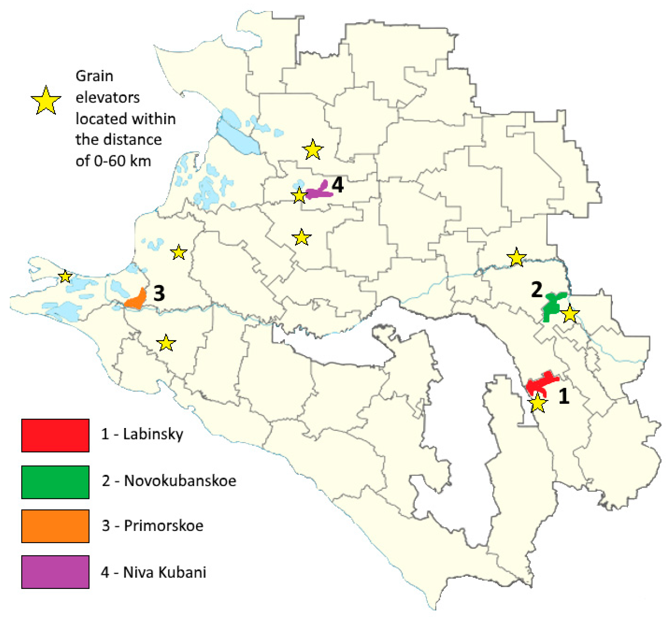
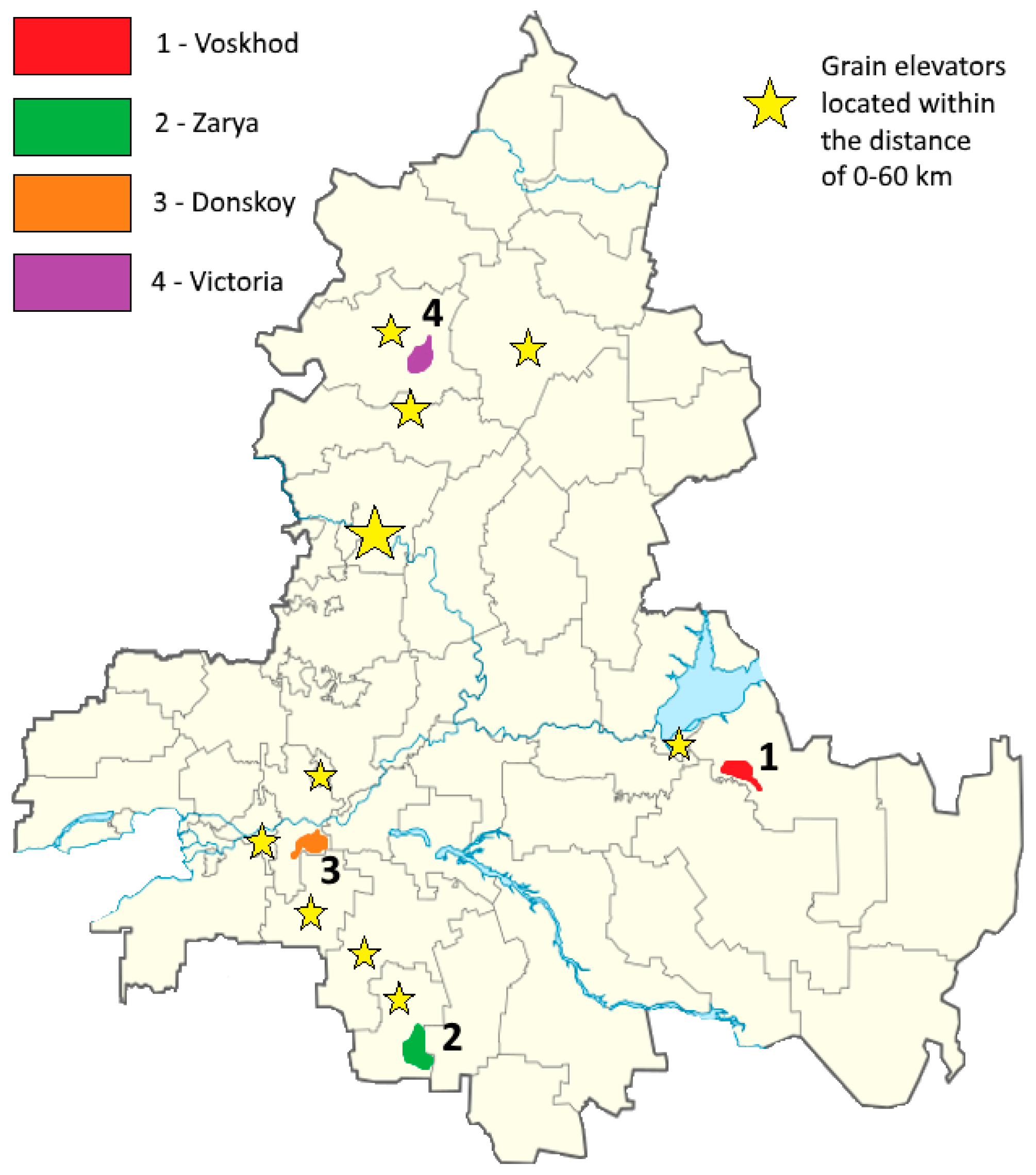
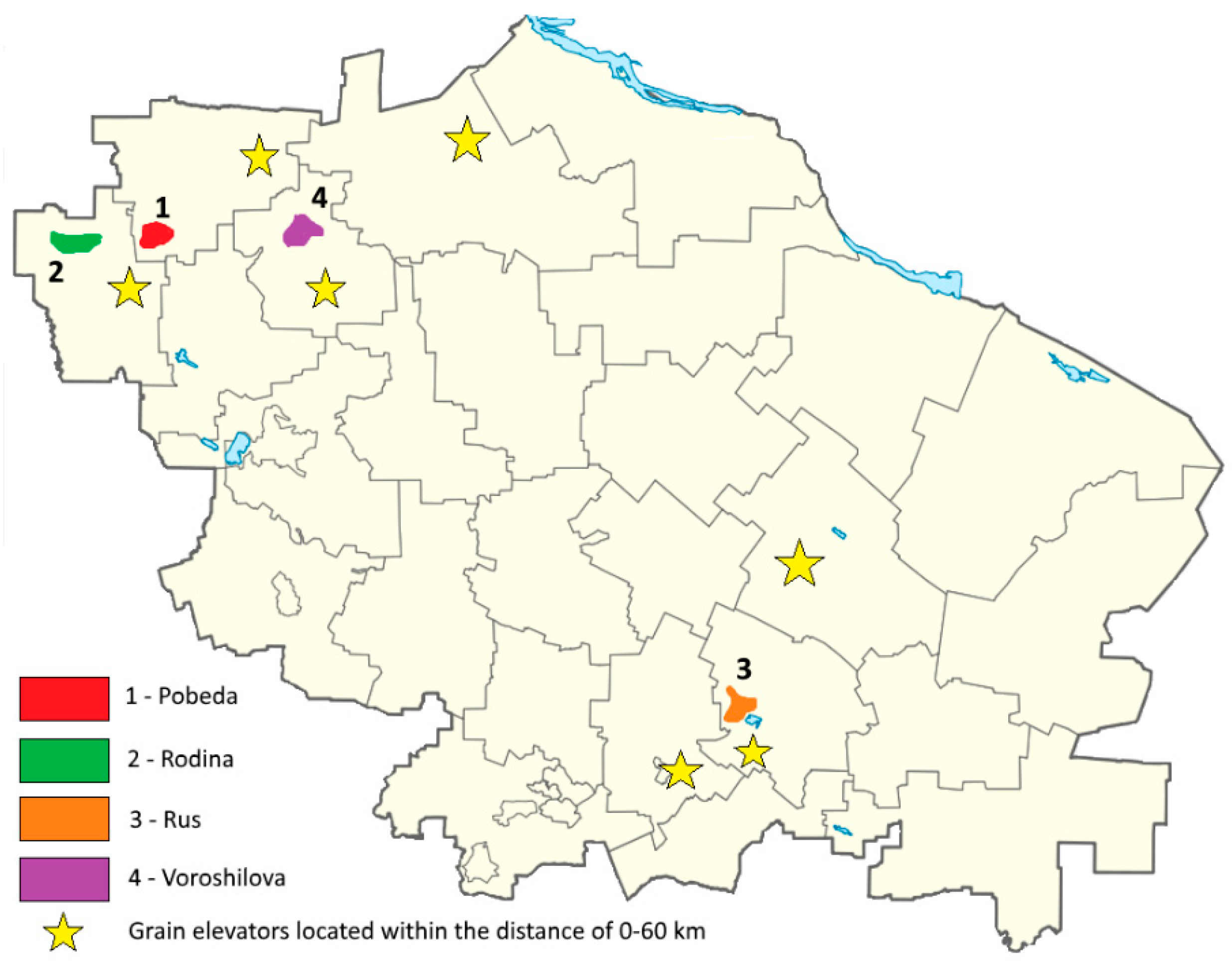
Source: authors’ development based on [9].
Table 3. Distance of transportation and volume of fuel required for the continuous operation of agricultural enterprises under study, average in 2013–2017.
TerritoryAgricultural EnterpriseTransportD1 kmD2 kmVs LVt L
Krasnodar regionLabinskyOwn10.44.275527186
NovokubanskoeOwn16.83.890818903
PrimorskoeOutsource67.210.763796088
Niva KubaniOutsource12.518.688127275
Rostov regionVoskhodOutsource83.121.413,22312,035
ZaryaOutsource22.312.650023581
DonskoyOwn9.42.442894016
VictoriaOwn88.032.715,60112,494
Stavropol regionPobedaOwn71.726.212,38810,290
RodinaOutsource67.614.510,99710,689
RusOutsource25.113.866185391
VoroshilovaOwn35.310.514,00912,589
Source: authors’ development.
Table 4. VsVt variations depending on the distance and the mode of transportation: grouping of agricultural enterprises.
GroupsD1Transport ModeAgricultural Enterprises/TerritoryVs–Vt Variation, Percentage
Group 10–60 kmOwnLabinsky/Krasnodar4.85
Novokubanskoe/Krasnodar1.96
Donskoy/Rostov6.37
Voroshilova/Stavropol10.14
Group 20–60 kmOutsourceNiva Kubani/Krasnodar17.44
Zarya/Rostov28.41
Rus/Stavropol18.54
Group 3>60 kmOwnVictoria/Rostov19.92
Pobeda/Stavropol16.94
Group 4>60 kmOutsourcePrimorskoe/Krasnodar4.56
Voskhod/Rostov8.98
Rodina/Stavropol2.80
Source: authors’ development.

