Analysis of Oil Price Effect on Economic Growth of ASEAN Net Oil Exporters

Abstract

In this paper, the linear and nonlinear effects of oil price on growth for Association of Southeast Asian Nations (ASEAN)—3 net oil-exporting countries, namely Brunei, Malaysia and Vietnam, are investigated. The empirical analysis applies the augmented autoregressive distributed lag model (ARDL) bound test approach and the nonlinear autoregressive distributed lag model (NARDL) methodology over the period of 1979 to 2017. Evidence suggests that ignoring nonlinearities may lead to misleading results. Specifically, results reveal that the effect of oil price is asymmetric for the case of Brunei, while the effect oil price is deemed insignificant for the case of Malaysia and Vietnam, both linear and nonlinear model. Brunei’s high dependency on oil revenue makes it susceptible to negative oil price shock. This suggests that oil price still plays a significant role as the main driver of economic progress for Brunei.

1. Introduction

Various studies have been conducted on the topic of oil. Oil has been a major interest to researchers because it is a significant limited resource whose price dynamics can affect the economy and the financial markets. Despite the ongoing race towards climate goals, along with the development and the advocating of electric cars and renewable energy sources, crude oil indisputably remains as one of the most important commodities in the global energy market. Furthermore, the price of crude oil is used as a benchmark for economic perspectives, currency movement, inflation and to determine the level of political unrest in the Middle East, thus making it one of the most critical global macro indicator [1]. Among the major studies conducted on oil are the impact of oil prices on exchange rate [2,3,4], the impact of oil price shocks on stock market [5,6,7] and also the impact of oil price shocks on other macroeconomic variables mainly GDP [8,9,10].

One of those research that is often the focal point for economic researchers in the field of crude oil is the effect of oil price on economic growth. In the pioneering works of Hamilton [11] in this field of research, it is discovered that every US recession that took place after World War II was partially induced by oil price increases. Based on previous works of literature, researchers will first segregate the countries based on whether it is an oil-exporting or oil-importing country. Depending on the researcher, they might want to conduct research exclusively on oil-exporting or oil-importing group of countries or even both, such as in the case of Su et al. [12]. Such identification is required because the changes in oil price affect an oil-exporting and oil-importing country differently. Consensus has it that an increase in oil price is generally favourable to oil-exporting countries but unfavourable for oil-importing countries. For instance, an increase in oil price for oil-exporting countries will lead to an increase in real gross domestic product [13], while an increase in oil price for the oil-importing country will lead to a decrease in the real gross domestic product (proxied by domestic industrial output) as shown by Qianqian [14]. Several empirical studies point towards a positive linear relationship between oil price and economic activities [15,16].

Even with the proliferation of studies on crude oil price, yet the number of studies on oil-exporting countries is still limited. On top of the limited studies on oil-exporting countries, most of it tends to focus on Organization of Petroleum Exporting Countries (OPEC) and Middle East countries, while studies on Association of Southeast Asian Nations (ASEAN) economies are limited. ASEAN consist of 10 Southeast Asian nations in which only three countries are deemed to be net oil exporters, namely Brunei, Malaysia and Vietnam (countries that have a consistent positive net oil exports from the year 2002 to 2016 is deemed as net oil exporters). This is reflected in

Table 1. Net oil exports of ASEAN countries (thousand barrels per day).

Year	Brunei	Cambodia	Indonesia	Laos	Malaysia	Myanmar	Philippines	Singapore	Thailand	Vietnam
2002	187.9	0	277.9	0	232.6	−6.9	−250.1	−816.4	−682.2	322.1
2003	196.0	0	192.1	0	235.6	0.6	−238.8	−938.2	−709.1	337.0
2004	186.5	0	103.3	0	217.7	0.0	−189.6	−1114.3	−815.7	388.6
2005	196.0	0	81.5	0	212.2	6.3	−199.7	−1176.8	−762.1	369.7
2006	196.9	0	−7.5	0	188.0	2.2	−202.0	−1150.1	−763.9	340.2
2007	171.2	0	56.5	0	144.7	2.9	−189.0	−1162.5	−752.2	328.9
2008	163.9	0	46.1	0	126.1	0.8	−172.5	−1158.0	−765.7	308.0
2009	141.9	0	46.5	0	158.3	0.9	−117.0	−871.8	−762.3	296.6
2010	147.6	0	76.1	0	164.0	0.0	−165.0	−944.0	−786.2	216.6
2011	135.4	0	96.2	0	49.9	−0.1	−171.5	−973.9	−761.7	182.4
2012	139.0	0	61.5	0	27.1	2.7	−162.5	−966.2	−819.2	183.0
2013	117.0	0	6.8	0	47.1	2.7	−140.1	−939.8	−843.2	165.7
2014	107.6	0	−40.8	0	38.6	2.8	−160.0	−942.0	−798.2	180.6
2015	115.5	0	−69.8	0	150.4	1.8	−197.9	−977.9	−818.3	183.6
2016	109.7	0	−61.8	0	192.5	2.7	−222.1	−1029.9	−842.2	148.9

Source: Energy Information Administration (EIA).

, which shows the net oil exports of each ASEAN countries using data, from 2002 to 2016, obtained from the Energy Information Administration [17]. The geographic location of the ASEAN oil-exporting countries is shown in Figure 1. Oil remains an essential resource for these oil-exporting countries from their contribution to the economy. The government revenue derived from petroleum or crude oil for Malaysia is at 29.04% of total government revenue for the year 2014 [18] and for Vietnam, oil revenue for 2014 was 11.04% of the total state budget revenue [19]. In the case of Brunei, the oil revenue for 2014/2015 was Brunei Dollar (BND) $5 690 million, which is 86.33% of the total government revenue [20], a higher reliance on oil as compared to the other two countries. Generally, oil revenue contributes a significant amount to the total government revenue. This figure would have been higher when the crude oil price was higher.

While a rise in oil price is associated with a contribution to the economic growth of oil-exporting countries through an increase in oil revenue, this may not always be the case. The economic growth might even be impaired as it might worsen the economic conditions favourable to economic growth via appreciation of exchange rates, rent-seeking and poor policy-making [21]. This indicates a possibility that a positive oil price shocks can have a detrimental effect on the economic activities of the ASEAN oil-exporting countries. As such, the oil price shocks on the economic activity of ASEAN oil-exporting countries could be asymmetric, and thus the assumption of the symmetric effect of oil price changes on the economic activity may not be accurate. For instance, Nusair [10] found that all six Gulf Co-operation Council countries examined indicate an asymmetric effect of oil price on economic activity to be present. Similarly, Donayre and Wilmot [22] found that during the recessionary period for Canada, the positive oil price shocks have a more substantial effect than the negative oil price shocks on the output and that this asymmetry is lessened during expansionary times. It is also worth noting that empirical evidence on asymmetric effects of oil price shocks on output was first provided by Mork [23].

Hence the objective of this paper is to examine the asymmetric effect of oil price on the economic activity of ASEAN oil-exporting countries. Using data from 1979 to 2017, the nonlinear autoregressive distributed lag model (NARDL) of Shin et al. [24] approach is employed to ascertain the existence of asymmetry in both the short-run and long-run.

This study provides several unique contributions to a growing body of literature on oil price and economic growth in three aspects. First, studies discerning the oil shocks (i.e., positive and negative) are limited and, in the process, implicitly assumed changes in oil prices to have symmetric effects on macroeconomic activities, including economic growth. Therefore, this study attempts to validate the existence of a nonlinear relationship between oil price and economic growth, using the newly developed NARDL model developed by Shin et al. [24]. Second, previous studies on ASEAN countries focus on a bivariate relationship, between oil price and economic growth, which results in the potentially misspecified model (see Aziz and Dahalan [25]). When some relevant explanatory variables are omitted from the regression, the results from the model could be biased. This issue is sometimes referred to as variable omission bias. Thus, this study circumvents such potential issues by incorporating control variables (i.e., life expectancy, population and gross fixed capital formation), which may potentially explain the sophisticated oil price and economic growth relationship adequately. Third, most studies provide emphasis on panel studies, which stressed on major oil exporters such as the Gulf Cooperation Council (GCC) countries, the Organization of the Petroleum Exporting Countries (OPEC) countries and also ASEAN-5. However, empirical studies using time series technique to study the nonlinear effect is mainly limited. Employing a single country analysis provides the ability to incorporate the heterogeneity issue of the distinctive character of a particular country. Hence this study evades the assumptions of homogeneity across countries in various aspects [26]. Fourth, this study will contribute to the limited studies on nonlinearity of oil-exporting countries.

The remainder of this paper is organised as follows: Section 2, reviews the strands of oil price–economic growth literature relevant to this study. Section 3 presents the empirical model and outlines the estimation procedures. In Section 4, the estimation results are presented. Finally, Section 5 summarises the key findings with recommendations on potential measures.

2. Literature Review

The impact of crude oil price on economic growth has most certainly, drawn much attention from researchers, especially during times of crisis. One notable oil price crisis occurred during the year 1973, due to the OPEC embargo. An embargo on oil exports to selected countries deemed as pro-Israel were announced by Arab oil-producing countries of OPEC. Furthermore, total oil productions by the OPEC was also cut back. Despite Iran increasing its production of oil, only a small part of it was offset. As a result, there was a shortage of crude oil, resulting in an oil price shock. Following the oil embargo, the US undergo a recession that started in November 1972. This oil crisis has highlighted the need for an in-depth analysis of the crude oil nexus.

Early studies conducted on the effect of oil prices on macroeconomic variables has spurred the research on oil prices [11,27,28,29]. Notably, one of the eminent research by Hamilton [11], found that increases in oil prices after World War II has played a partial role in inducing every US recessions that occurred. Overall, early studies conducted by these researchers found a negative relationship between oil price and economic growth. However, most of these studies focus mainly on the impact of crude oil price shocks in the context of a net oil-importing countries and thus studies on net oil-exporting countries are limited [30].

Furthermore, most past studies implicitly assumed that the effect of oil price on economic growth is linear. However, this may not necessarily be the case, as most macroeconomic variables have nonlinear characteristics [31]. True enough, the linear estimation begins to lose its significance later on, by the mid-1980s [32]. One of the first empirical studies that focus on the asymmetric effects of oil price shocks on output was spurred by Mork [23]. This study found that positive oil price changes have a significantly strong negative relationship with changes in the real GNP, while a negative oil price change is deemed insignificant. As such, it can be concluded that the asymmetric effect exists and, in that process, invalidating the linear effect. More importantly, the study by Mork [23] has laid the foundations for subsequent studies on the asymmetric effect of oil price on various other macroeconomic variables.

One of the earliest theories on the asymmetric effect of oil price on the economic activity of oil-exporting countries can be traced back to the Dutch disease theory [33]. Accordingly, there is a decrease in manufacturing output for resource-rich countries. During the higher oil price period, oil-exporting countries will shift the structure of their economy away from traded manufacturing and agriculture sectors towards booming oil and nontraded sectors instead, resulting in detrimental effects. Moreover, an appreciation of the local currency as a result of increased oil revenues will lead to increased imports of intermediate and consumer goods. This increased reliance on imported goods will then harm domestic industries as they are not able to compete when oil prices are high and are unable to sustain their production levels when oil prices and imports decline. Hence, a temporary exchange rate appreciation will be detrimental towards the economy rather than benefiting it based on Dutch disease theory. A decline in oil prices will have the opposite effect instead. Empirically, some findings do not seem to support this theory. For instance, Ito [34] found that the Dutch disease is not supported for Russia. In regards to exchange rate appreciation as a result of oil price hike, Korhonen and N. Mehrotra [35] determined that oil shocks do not account for a large share of movements in the real exchange rate. They concluded that supply shocks are the most important factor driving the real output in the four oil-exporting countries.

Another theory on the asymmetric effect of oil price on economic growth was posited by Moshiri and Banihashem [21], in which government size and their excessive intervention in those countries play a pivotal role in explaining the asymmetry. In this theory, the government revenue derived from crude oil is used in driving the economic activities of those countries. Due to these countries often adopting procyclical fiscal policies, the government often spends aggressively on physical capital development and social projects when oil prices are high but does not often contribute much to the economy due to poor management, rent-seeking behaviour and lack of transparency, and competition. When the oil prices fall sharply, most economic activities are halted, and massive investment projects are left incomplete. Thus, given that the country is not able to reap wholly the benefit that often accompanies high oil prices as much as the negative effect of low oil prices, thus an asymmetric effect is present.

Empirically, several researchers were able to determine the existence of the asymmetric effect. By examining the effect of oil price on the economic activity of the Gulf Co-operation Council countries, Nusair [10] found that asymmetric effect was present in all six countries. Similarly, Donayre and Wilmot [22] and Farzanegan and Markwardt [30] also found an asymmetric effect in their studies. As for the case of ASEAN countries, Aziz and Dahalan [25] used a panel VAR model for the ASEAN-5 countries consisting of Indonesia, Malaysia, Philippines, Singapore and Thailand. Overall the studies suggest asymmetric effect for the case of ASEAN-5. However, the response of GDP to oil price was found to be negative. This is, not surprising as a panel data approach is used, and not all the countries will react the same to a change in oil price. Kose and Baimaganbetov [36] who found the asymmetric effect to be present in Kazakhstan, suggest that income derived from oil revenues should be invested in the tradable goods sector and social infrastructure to promote economic growth and sustainable development. However, in some cases, there are countries where the oil price shocks effect on GDP growth is linear such as in the case of Iran and Kuwait [21].

3. Results

3.1. Empirical Model

With a plethora of growth studies available, the endogenous growth model is employed, where GDP per capita is used to measure growth. The use of GDP per capita provides a more comparative measure of living standards as opposed to total GDP. With regards to the endogenous growth theory, there are several numbers of variables that are significantly correlated with growth regression models, including but not limited to initial level of income, investment rate, various measures of education and certain policy indicators [37,38]. Furthermore, based on the work of Aziz and Dahalan [25], Donayre and Wilmot [22], and Nusair [10], it is apparent that oil price also plays an important role in the determination of the economic growth of net oil-exporting countries. In line with that, the following multivariate specification is employed, as inspired by the growth regression model, which is broadly similar to Levine and Renelt [39], Campos [40], and Azman-Saini et al. [41], with the addition of oil price as an explanatory variable:

$$LnGDPP{C}_t=a+bLnBREN{T}_t+cLnL{E}_t+dLnPO{P}_t+eLnGFC{F}_t+{\epsilon }_t$$

(1)

where LnGDPPC denotes the natural log of real gross domestic product per capita, LnBRENT denotes the natural log of real Brent crude oil price, LnLE denotes natural log of life expectancy, LnPOP denotes natural log of total population as a measure of the labour force, and LnGFCF denotes natural log of real gross fixed capital formation as a measure of investment.

The Brent crude oil price is used to proxy for oil price as 70% per cent of international trade in oil is directly or indirectly priced from the Brent basket, making Brent the main price benchmarks for crude oil [42]. Furthermore, several studies on oil-exporting countries also favoured Brent crude oil price in their research [43,44]. The estimate for b, in this case, could be positive as mentioned earlier as oil exporting country often gains from an increase in crude oil price. This scenario is primarily because, in oil-exporting countries, part of the government’s revenue consists of oil revenue. Thus, when the oil price increase, the oil revenue will also increase due to the higher oil price. As such, the government can invest the extra revenue obtained from the increase in the oil price to develop the country and in the process, contribute to economic growth.

Life expectancy is used as a measure of human capital following the work of Azman-Saini et al. [41] and Hajamini and Falahi [45], which is often viewed as one of the main drivers of economic growth in the development of economics literature [46,47,48]. A more productive labour force as a result of adequate education and good health will stimulate national economic growth [49]. Hence, a positive coefficient estimate is expected for life expectancy in the growth model.

On the other hand, labour growth, which is a critical determinant of growth [50], is proxied by the total population in this case. When population increases, it translates to a reduction in the capital/labour ratio because capital must now be distributed more thinly across the bigger population of workers, thus affecting GDP per capita negatively [48].

Similarly, LnGFCF is used to proxy for the capital stock, which is an essential component of the production function. LnGFCF leads to influence the multifactor productivity and hence the production indirectly, resulting in higher productivity and efficiency [51]. Therefore, a positive coefficient estimate, e, is expected for LnGFCF.

As noted earlier, the effect of oil price on economic growth could be asymmetric. Hence, to examine the asymmetric effect of oil price on the economic growth of the oil-exporting countries of ASEAN, the NARDL model of Shin et al. [24] will be employed, which is an extension of Pesaran et al. [52] linear ARDL bound testing approach. However, the linear ARDL model is first estimated before the NARDL model to determine if the oil price is deemed significant in a linear context.

There are several advantages in employing an ARDL model to estimate the linear effect of oil price on economic growth. The first advantage is the variables could be integrated of order zero, one or a combination of both, and the results yield remains valid. In other words, an ARDL model can be used to determine the presence of a long-run relationship among variables despite having a different order of integration of variables, unlike other cointegration tests which require that all the variables are of the same order of integration. Second, the ARDL model is suitable for this research as it performs better when estimating small sample sizes compared to other cointegration tests [53].

The models proposed above are long-run models, and as such, its coefficient estimates only the long-run effects. Thus, the equations shall be reparameterized into an unrestricted error-correction modelling format. The following error-correction models shall be used along with the Pesaran et al. [52] bound testing approach.

$$\begin{array}{ll}\Delta LnGDPP{C}_t=\alpha & +{\displaystyle \sum _{k=1}^{n1}}{\beta }_k\Delta LnGDPP{C}_{t-k}+{\displaystyle \sum _{k=0}^{n2}}{\delta }_k\Delta LnBREN{T}_{t-k}+{\displaystyle \sum _{k=0}^{n3}}{\phi }_k\Delta LnL{E}_{t-k}\\ & +{\displaystyle \sum _{k=0}^{n4}}{\theta }_k\Delta LnPO{P}_{t-k}+{\displaystyle \sum _{k=0}^{n5}}{\pi }_k\Delta LnGFC{F}_{t-k}+{\lambda }_{1}LnGDPP{C}_{t-1}\\ & +{\lambda }_{2}LnBREN{T}_{t-1}+{\lambda }_{3}LnL{E}_{t-1}+{\lambda }_{4}LnPO{P}_{t-1}+{\lambda }_{5}LnGFC{F}_{t-1}\\ & +{\lambda }_{6}DUMMY+{\mu }_t\end{array}$$

(2)

where Δ denotes the first different operator, DUMMY is the dummy variable to account for a possible structural break, and μ_t represents the white noise residuals.

Based on the equations above, one observable advantage is that both the short-run and long-run estimates are provided at once within a single equation framework. The short-run effects will be the estimates of the coefficient for each first differenced while the long-run effect will be the estimates of λ² to λ⁵ normalise on λ¹ for Equation (3). However, the long-run estimates are meaningful only if cointegration can be established. There are three separate tests to establish the existence of cointegration among the variables, namely, the F-test for joint significance of lagged variables and the t-test on the lagged level of the dependent variable as suggested by Pesaran et al. [52] and another additional F-test on the lagged levels of the independent variable(s) as suggested by McNown et al. [54].

In the F-test for joint significance of lagged variables, also known as a bound test, the calculated F-statistic is compared with the lower bound and the upper bound. Should the F-statistic be below the lower bound, the null hypothesis of no long-run relationship cannot be rejected while an F-statistic that is greater than the upper bound means that the null hypothesis can be rejected, signifying the existence of a long-run relationship. However, if the F-statistic falls between the lower and upper bound, the result is said to be inconclusive. Even though the cointegration analysis using the ARDL model is suitable for small sample studies such as this, the critical values provided by Pesaran et al. [52] are generated with a sample size of 1000 observations along with 40,000 replications. As such, this study will instead use the Narayan [55] critical value for the lower bound and the upper bound. The Narayan [55] critical values provide the lower bound and the upper bound value for small sample sizes ranging from 30 to 80 with a 5-observation interval in between and have been generated with 40,000 replications as well.

An issue that arises from the F-test, however, is whether the significance of the test arises merely from either the lagged level of the dependent variable or the lagged level of the independent variable(s) alone. As such, performing a t-test is necessary to rule out the possibility of a degenerate lagged dependent variable case. One of the assumptions made by Pesaran et al. [52] is the dependent variable must I(1), which rules out degenerate lagged independent variable(s) case. The idea behind this is that the ARDL equation will be similar to a generalised Dickey–Fuller equation when the lagged level dependent variable is deemed significant. A significant lagged dependent variable indicates that the dependent variable is integrated of order zero, i.e., I(0). One notable issue that should be stated here is the lack of small sample critical value bounds for the t-statistic. Narayan [55] only provided small sample critical values for the F-test for the joint significance of lagged variables and not the small sample critical value bounds for the t-test of the lagged dependent variable. As such, the t-test on the lagged level dependent variable for this study will use the Pesaran et al. [52] critical value that is reported on [52]. As with the earlier F-test on the joint significance of lagged variables, if the computed t-statistic exceeds the upper bound critical value, this study can establish statistical significance.

In addition to the two-test mentioned above, an F-test on the lagged levels of the independent variable(s) introduced by McNown et al. [54] is employed. This additional test will circumvent the presumption of the dependent variable to be I(1). As such, the use of such additional test will minimise the risk of false conclusions made from standard unit root tests, which are notorious for their low power. Like the bound test proposed by Pesaran et al. [52], the F-statistic obtained from this test will refer to the critical values tabulated by Sam et al. [56], which consist of a lower bound as well as an upper bound. If the F-statistic exceeds (lower than) the upper bound, the null hypothesis is rejected (accepted), and the test is significant (insignificant). If the F-statistic falls between the bounds, the test is inconclusive. Integrating this test with the two-test proposed by Pesaran et al. [52] will provide a clearer picture of the system’s cointegration status. This new method of determining cointegration is coined as the augmented ARDL bounds test. The null hypothesis and the alternative hypothesis for all three tests are summarised in

Table 2. Null and alternative hypothesis for the three cointegration test.

Cointegration Test	Null Hypothesis	Alternative Hypothesis
F-bound test	${\lambda }_1={\lambda }_2={\lambda }_3={\lambda }_4={\lambda }_5=0$	$any {\lambda }_1,{\lambda }_2,{\lambda }_3,{\lambda }_4,{\lambda }_5\ne 0$
t-test on lagged dependent variable	${\lambda }_1=0$	${\lambda }_1\ne 0$
F-test on lagged independent variable	${\lambda }_2={\lambda }_3={\lambda }_4={\lambda }_5=0$	$any {\lambda }_2,{\lambda }_3,{\lambda }_4,{\lambda }_5\ne 0$

.

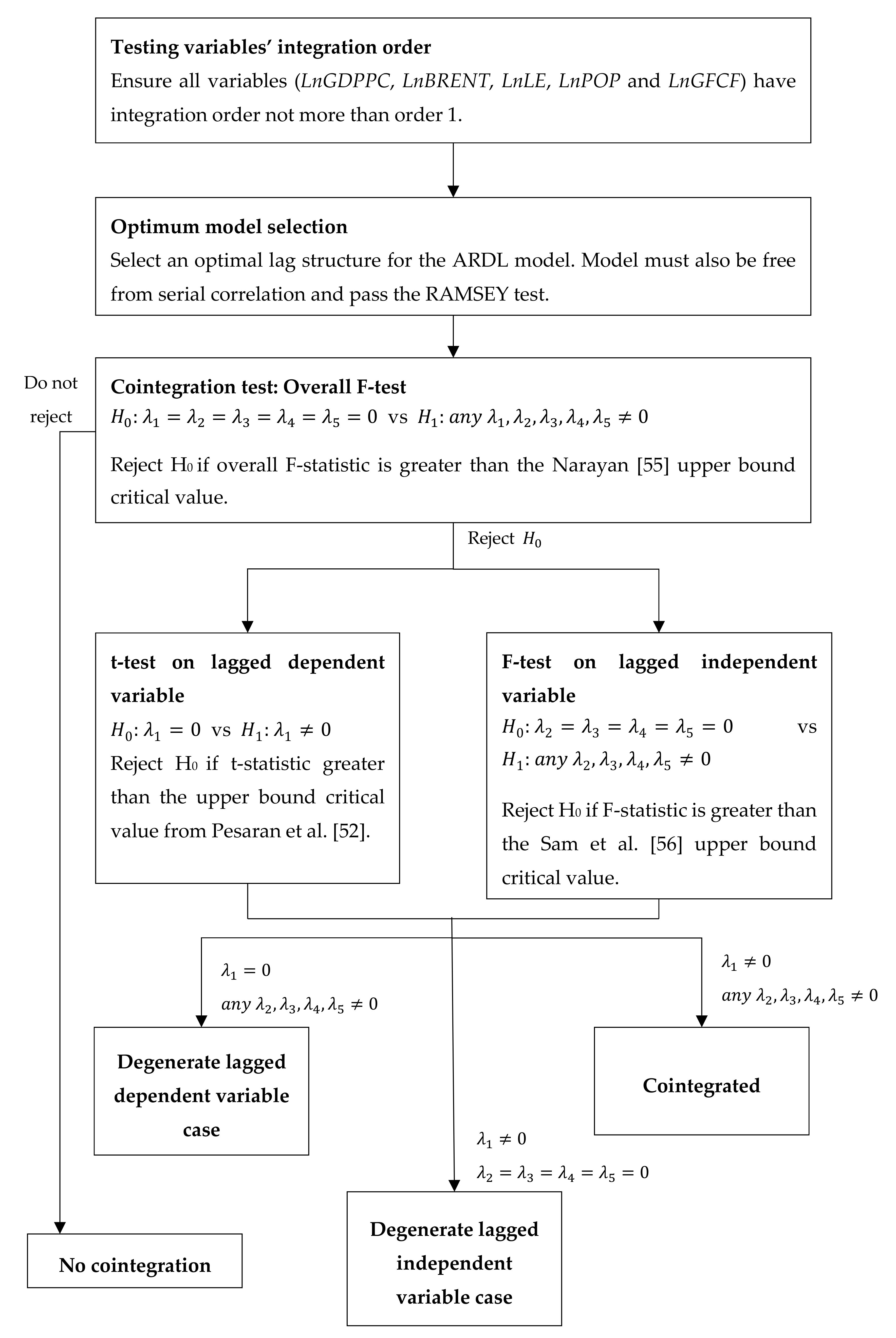
There are four probable outcomes based on the results obtained from the three cointegration test mentioned. The first outcome is when the F-test for joint significance of lagged variables and the F-test on the lagged levels of the independent variable(s) are significant, but the t-test on the lagged dependent variable is insignificant. This outcome is known as degenerate lagged dependent variable or degenerate case #1 (See McNown et al. [54], Goh et al. [57]). The second outcome is when the F-test for joint significance of lagged variables and the t-test on the lagged level dependent variable is significant, but the F-test on the lagged level of the independent variable(s) are insignificant. This outcome is coined as degenerate lagged independent variable or degenerate case #2. The third outcome occurs when the F-test for the joint significance of lagged variables is insignificant. The fourth outcome is when all three tests are found to be significant. The first and second outcome are degenerate cases and, along with the third outcome, would imply no cointegration. Only the fourth outcome will imply cointegration among the variables. The four outcomes are summarised in

Table 3. Summary of four outcomes from the three cointegration test.

Outcome	F-Bound Test	t-Test on Lagged Dependent Variable	F-Test on Lagged Independent Variable	Conclusion
1	✓	✗	✓	Not cointegrated (Degenerate case #1)
2	✓	✓	✗	Not cointegrated (Degenerate case #2)
3	✗	Not necessary	Not necessary	Not cointegrated
4	✓	✓	✓	Cointegrated

Note: ✓ refers to significant test statistic and ✗ refers to an insignificant test statistic

for convenience purpose, and the procedures for the implementation of the augmented ARDL bounds test is summarised in Figure 2 (See Sam et al. [56]).

To test the asymmetric assumption, which is postulated, the NARDL model, which is an asymmetric expansion of the linear ARDL model, is employed. This methodology allows the decomposition of the independent variables into both positive and negative partial sum of processes to investigate the nonlinear characteristics.

$$POS={\displaystyle \sum }_{j=1}^t\Delta OI{L}_j^{+}={\displaystyle \sum }_{j=1}^t\max \left(\Delta BREN{T}_j,0\right),$$

$$NEG={\displaystyle \sum }_{j=1}^t\Delta OI{L}_j^{-}={\displaystyle \sum }_{j=1}^t\min \left(\Delta BREN{T}_j,0\right),$$

where POS and NEG are partial sum processes of positive and negative changes in BRENTt, respectively. Replacing BRENTt variable with POS and NEG, the specifications are

$$\begin{array}{ll}\Delta LnGDPP{C}_t=\alpha & +{\displaystyle \sum _{k=1}^{n1}}{\beta }_k\Delta LnGDPP{C}_{t-k}+{\displaystyle \sum _{k=0}^{n2}}{\delta }_k^{+}\Delta PO{S}_{t-k}+{\displaystyle \sum _{k=0}^{n3}}{\delta }_k^{-}\Delta NE{G}_{t-k}\\ & +{\displaystyle \sum _{k=0}^{n4}}{\phi }_k\Delta LnL{E}_{t-k}+{\displaystyle \sum _{k=0}^{n5}}{\theta }_k\Delta LnPO{P}_{t-k}+{\displaystyle \sum _{k=0}^{n6}}{\pi }_k\Delta LnGFC{F}_{t-k}\\ & +{\lambda }_{1}LnGDPP{C}_{t-1}+{\lambda }_{2}PO{S}_{t-1}+{\lambda }_{3}NE{G}_{t-1}+{\lambda }_{4}LnL{E}_{t-1}\\ & +{\lambda }_{5}LnPO{P}_{t-1}+{\lambda }_{6}LnGFC{F}_{t-1}+{\lambda }_{7}DUMMY+{\mu }_t\end{array}$$

(3)

Given that the NARDL model is an extension of the ARDL model, the NARDL model will also be subjected to the conditions under an ARDL model. In this case, the NARDL model will need to undergo the three cointegration test required under an augmented ARDL model to determine if cointegration exists.

Once the long-run relationship between the variables has been established, the potential for asymmetric effect shall then be investigated. To test for the short-run symmetry, a Wald test under the null hypothesis of $H_0:{{\displaystyle \sum }}_{k=0}^{n2}{\delta }_k^{+}={{\displaystyle \sum }}_{k=0}^{n3}{\delta }_k^{-}$. Similarly, the long-run symmetry is tested under the null hypothesis of ${\lambda }_2={\lambda }_3$.

This section may be divided by subheadings. It should provide a concise and precise description of the experimental results, their interpretation as well as the experimental conclusions that can be drawn.

3.2. Data and Sources

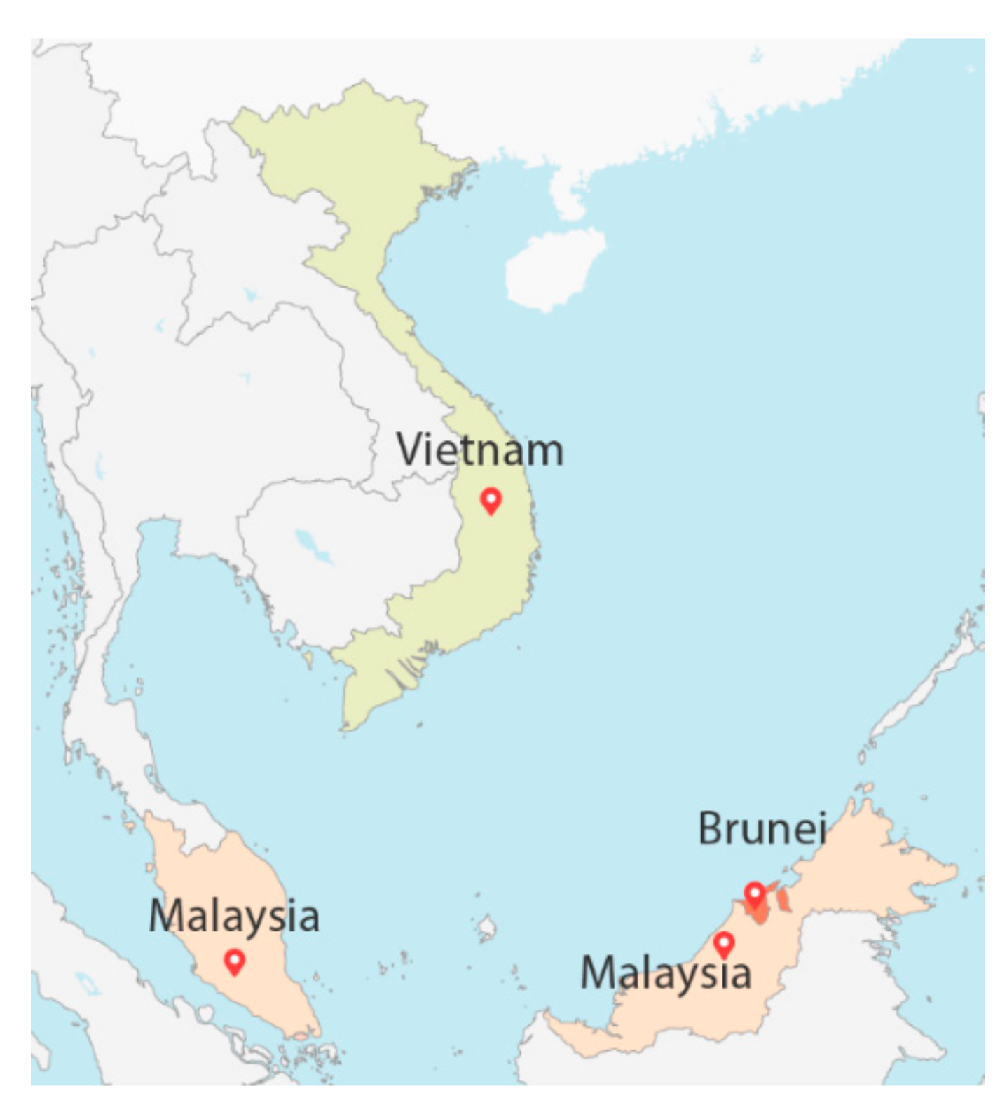
This study employs annual data with the sample period ranging from 1979 to 2017. The real gross domestic product per capita is derived by obtaining the real gross domestic product from the United Nations Statistics Division (UNSD) and dividing it by the total population obtained from the World Development Indicator (WDI). The Brent crude oil price is extracted from the World Bank Commodity Price Data (WBC). Total population and the life expectancy data are obtained from WDI while the gross fixed capital formation is obtained from UNSD. Descriptions of the data are summarised in

Table 4. Sources of data.

Variables	Descriptions	Measurement	Sources	Expected Sign
GDPPC	Real Gross Domestic Product Per Capita	Constant US Dollar 2010	UNSD, WDI
BRENT	Brent crude oil price (USD/Barrel)	Constant US Dollar 2010	WBC	+
LE	Life Expectancy	Years	WDI	+
POP	Total Population	Total number	WDI	−
GFCF	Gross Fixed Capital Formation	Constant US Dollar 2010	UNSD	+

Notes: WDI: World Development Indicator; UNSD: United Nations Statistics Division; WBC: World Bank Commodity Price Data.

below.

Table 5. Descriptive statistics (before log transformation).

Variable	Mean	Min	Max	Std. Dev
Brunei
GDPPC	39,588.59	31,430.74	72,437.55	8,450.31
BRENT	47.34	15.48	101.58	26.19
LE	74.38	69.94	77.37	2.31
POP	313,146.36	187,656.00	428,697.00	74,438.09
GFCF	2.80 × 109	9.23 × 108	6.39 × 109	1.40 × 109
Malaysia
GDPPC	6,673.06	3,194.60	11,528.34	2,481.98
BRENT	47.34	15.48	101.58	26.19
LE	72.07	67.73	75.45	2.23
POP	22,179,506.21	13,460,201.00	31,624,264.00	5,634,228.05
GFCF	4.09 × 1010	9.12 × 109	9.27 × 1010	2.39 × 1010
Vietnam
GDPPC	817.49	309.52	1,834.65	462.11
BRENT	47.34	15.48	101.58	26.19
LE	72.35	66.88	76.45	2.79
POP	76,286,359.77	53,169,673.00	95,540,800.00	12,601,992.94
GFCF	1.67 × 1010	1.39 × 109	5.42 × 1010	1.59 × 1010

provides the descriptive statistic for the variables employed in the estimation before the log transformation. Throughout the 39 years, the minimum GDPPC for Brunei was 31,430.74 while the maximum GDPPC is 72,437.55 USD, with an average of 39,588.59 USD. From this average, the changes in the GDPPC were around plus or minus 8,450.31 USD. The BRENT crude oil price ranges from a minimum of 15.48 USD to 101.58 USD, averaging 47.34 USD. The standard deviation for BRENT is 26.19 USD. For Malaysia, the minimum GDPPC is 3,194.60 USD, while the maximum GDPPC is 11,528.34 USD, averaging 6,673.06 USD. The changes in the GDPPC were around plus or minus 2,481.98 USD. As for Vietnam, the minimum GDPPC is 309.52 USD while the maximum GDPPC is 1,834.65 USD, averaging 817.49 USD. Changes in the GDPPC for Vietnam were around plus or minus 462.11 USD.

Table 6. Descriptive statistics (after log transformation).

Variable	Mean	Min	Max	Std. Dev
Brunei
LnGDPPC	10.57	10.36	11.19	0.18
LnBRENT	3.71	2.74	4.62	0.57
LnLE	4.31	4.25	4.35	0.03
LnPOP	12.62	12.14	12.97	0.25
LnGFCF	21.63	20.64	22.58	0.51
Malaysia
LnGDPPC	8.73	8.07	9.35	0.39
LnBRENT	3.71	2.74	4.62	0.57
LnLE	4.28	4.22	4.32	0.03
LnPOP	16.88	16.42	17.27	0.26
LnGFCF	24.24	22.93	25.25	0.67
Vietnam
LnGDPPC	6.55	5.74	7.51	0.57
LnBRENT	3.71	2.74	4.62	0.57
LnLE	4.28	4.20	4.34	0.04
LnPOP	18.14	17.79	18.38	0.17
LnGFCF	22.92	21.05	24.72	1.26

provides the descriptive statistics for the variables after log transformation.

Furthermore, this study employs the Pearson correlation coefficient to determine the existence of contemporaneous relationships among the variables. Before the correlation analysis is conducted, all variables are transformed using the log transformation. Results are reported in

Table 7. Pearson correlation results.

Variable	LnGDPPC	LnBRENT	LnLE	LnPOP	LnGFCF
Brunei
LnGDPPC	1.000
LnBRENT	−0.062	1.000
LnLE	−0.833 ***	0.370 **	1.000
LnPOP	−0.833 ***	0.374 **	0.998 ***	1.000
LnGFCF	−0.793 ***	0.172	0.831 ***	0.846 ***	1.000
Malaysia
LnGDPPC	1.000
LnBRENT	0.429 ***	1.000
LnLE	0.988 ***	0.365 **	1.000
LnPOP	0.992 ***	0.420 ***	0.997 ***	1.000
LnGFCF	0.969 ***	0.329 **	0.945 ***	0.941 ***	1.000
Vietnam
LnGDPPC	1.000
LnBRENT	0.540 ***	1.000
LnLE	0.975 ***	0.384 **	1.000
LnPOP	0.961 ***	0.329 **	0.998 ***	1.000
LnGFCF	0.984 ***	0.459 ***	0.986 ***	0.978 ***	1.000

Notes: N = 39. ***, **,* corresponds to 1%, 5%, and 10% significance level respectively (p-values are based on two-tailed tests).

. As shown in the table, LnBRENT shows a significantly positive contemporaneous correlation with LnGDPPC. Specifically, the mean of the Pearson correlation is 0.429 and 0.540 for Malaysia and Vietnam, respectively. These results are in line with the theoretical prediction, where an increase in oil prices improves the economy of an oil-exporting country. However, for the case of Brunei, the LnBRENT does not appear to have any significant contemporaneous correlation with LnGDPPC. These results, however, are merely correlation analysis and does not imply causation. A simple correlation which analyses the relationship between two variables will potentially disregard important explanatory variables. As such, a regression is required to ascertain the relationship between the variables.

4. Empirical Results

4.1. Unit Root Tests

Given that a cointegrating relationship between economic growth and oil price may exist, the augmented ARDL bound testing approach is employed to ascertain this relationship. However, for the augmented ARDL bound test to be applied, all the variables in the regression must achieve stationarity at I(0), I(1), or a mixture of both. Hence, to determine the stationarity of the variables used, the Zivot and Andrews [58] unit root test is employed in favour of the more common unit root test like the Augmented Dickey–Fuller (ADF) and Kwiatkowski–Phillips–Schmidt–Shin (KPSS) unit root test. The Zivot and Andrews [58] unit root test is superior as it accounts for structural breaks within the variables. Ignoring existing breaks leads to bias due to the reduction in the ability to reject a false unit root hypothesis [59]. The ASEAN countries and oil price in general, have undergone several episodes of economic crisis, which may lead to a structural break in the series (ASEAN countries have undergone the Asian Financial Crisis 1997, the financial crisis of 2007–2008 while oil price have several shocks mainly the 1980–1986: Iran-Iraq War, 1990–1991: First Persian Gulf War, 2003: Iraq War). Selection of the break date for Zivot and Andrews [58] test is based on where the t-statistic of the ADF unit root test is the smallest. When the t-statistic is higher than the Zivot and Andrews [58]’s critical values (in absolute value), the null hypothesis of nonstationarity can be rejected. The three models proposed by Zivot and Andrews [58] are Model A, Model B and Model C, whereby Model A allows for one-time change in the mean of the series, Model B allows for one-time change in the slope of the trend function and Model C allows for one-time changes in both the mean and the slope of the trend function. As with most unit root test, the structural unit root test is applied on the level and first differences of the variables. As observed from

Table 8. Zivot and Andrews [49]’s breakpoint unit root test results.

Variable	Level Variables			First Differenced Variables
	Model A	Model B	Model C	Model A	Model B	Model C
Brunei
LnGDPCC	−5.75(0) a [1986]	−4.52(0) b [2011]	−4.87(0) c [1986]	−6.07(0) a [1987]	−6.59(0) a [1992]	−6.49(0) a [1991]
LnBRENT	−3.12(0) [1986]	−2.95(0) [1987]	−3.21(0) [1986]	−6.61(0) a [2009]	−6.69(0) a [2006]	−6.99(0) a [1999]
LnLE	0.41(2) [2005]	−3.73(2) [2002]	−3.71(2) [2001]	−6.89(2) a [2005]	−4.39(2) a [2002]	−5.51(2) b [2005]
LnPOP	−3.15(2) [2003]	−5.20(2) a [1998]	−5.19(2) b [1998]	−2.52(2) [2002]	−1.66(2) [2008]	−2.64(2) [2002]
LnGFCF	−4.34(0) [1999]	−2.63(0) [1992]	−4.51(0) [1999]	−7.34(0) a [1997]	−6.35(0) a [2000]	−7.22(0) a [1997]
Malaysia
LnGDPCC	−3.46(0) [1991]	−2.54(0) [1996]	−3.40(0) [1991]	−6.35(0) a [1998]	−5.16(0) a [1992]	−6.31(0) a [1998]
LnBRENT	−3.12(0) [1986]	−2.95(0) [1987]	−3.21(0) [1986]	−6.61(0) a [2009]	−6.69(0) a [2006]	−6.99(0) a [1999]
LnLE	−9.42(2) [2001]	−4.85(2) b [1993]	−4.66(2) [1990]	−3.36(2) [2008]	−6.00(2) a [2005]	−6.83(2) a [2001]
LnPOP	−0.78(2) [1991]	−5.17(2) a [1994]	−4.70(2) [1992]	−5.84(2) a [1999]	−4.84(2) b [2011]	−5.11(2) b [2009]
LnGFCF	−3.64(1) [2001]	−3.25(1) [1995]	−4.25(1) [1998]	−5.08(0) b [1998]	−4.28(0) c [1999]	−5.01(0) c [1998]
Vietnam
LnGDPCC	−3.40(2) [2000]	−4.91(2) b [1987]	−3.69(2) [1989]	−8.34(0) a [1992]	−5.95(0) a [2004]	−8.15(0) a [1992]
LnBRENT	−3.12(0) [1986]	−2.95(0) [1987]	−3.21(0) [1986]	−6.61(0) a [2009]	−6.69(0) a [2006]	−6.99(0) a [1999]
LnLE	−7.39(2) a [2002]	−7.11(2) a [1997]	−6.83(2) a [1996]	−2.78(2) [2011]	−4.12(2) c [2008]	−3.67(2) a [2008]
LnPOP	−3.06(2) [1987]	−6.55(2) a [1992]	−5.20(2) b [1991]	−3.65(2) b [1993]	−3.96(2) [2002]	−3.57(2) [1998]
LnGFCF	−5.34(0) b [1992]	−2.89(0) [2004]	−5.09(0) b [1992]	−9.73(0) a [1990]	−7.92(0) a [1994]	−9.55(0) a [1990]

Notes: ^a, ^b, and ^c corresponds to 1%, 5%, and 10% significance level respectively. The 1%, 5% and 10% critical values: −5.34, −4.80 and −4.58 for Model A; −4.93, −4.42 and −4.11 for Model B; and −5.57, −5.08 and −4.82 for Model C.

, none of the variables is I(2), and hence the estimation of the ARDL model may proceed. Moreover, the variables have a mixed order of integration, I(0) or I(1), which underlines the significance of using an ARDL bound testing approach to determine cointegration. The results from Table 8 suggest that the break dates for Brunei, Malaysia and Vietnam are 1986, 1998 and 1992, respectively.

4.2. ARDL Results: Linear Model

The linear ARDL is first estimated. For this study, the Akaike Information Criterion (AIC) is set as the selection criteria. A maximum lag of 4 will be imposed for both the dependent variable and the regressors, where possible, provided there is no degree of freedom issues. However, the number of lags will be reduced if the selected model has serial correlation issues, as suggested by Pesaran et al. [52]. Results are reported in

Table 9. Linear autoregressive distributed lag model (ARDL) estimation results and diagnostic checks.

Variable	Country
	Brunei	Malaysia	Vietnam
Panel A: Coefficient estimates of linear ARDL
Selected model	(1, 1, 2, 2, 2)	(1, 1, 0, 1, 2)	(3, 0, 0, 0, 0)
Constant	−56.32(15.80) a	2.40(5.86)	−0.19(2.74)
LnGDPPCt−1	−0.98(0.08) a	−0.52(0.13) a	−0.04(0.03)
LnBRENTt−1	−0.03(0.02)	−0.01(0.01)	0.004(0.01)
LnLEt−1	26.40(5.88) a	−3.69(2.74)	−0.20(2.41)
LnPOPt−1	−3.62(0.79) a	0.90(0.38) b	0.05(0.43)
LnGFCFt−1	−0.05(0.03)	0.12(0.03) a	0.02(0.02)
∆LnGDPPCt−1			0.56(0.17) a
∆LnGDPPCt−2			−0.26(0.11) b
∆LnBRENTt	−0.01(0.02)	0.02(0.01)	0.004(0.01)
∆LnLEt	153.90(46.23) a	−3.69(2.74)	−0.20(2.41)
∆LnLEt−1	−206.89(48.57) a
∆LnPOPt	−44.53(10.75) a	−3.20(1.74) c	0.05(0.43)
∆LnPOPt−1	44.71(10.03) a
∆LnGFCFt	0.03(0.02)	0.17(0.03) a	0.02(0.02)
∆LnGFCFt−1	0.04(0.02) c	−0.06(0.02) a
DUMMY	−0.20(0.02) a	−0.02(0.02)	0.01(0.01)
Panel B: Diagnostic results
ECTt−1	−0.98(0.07) a	−0.52(0.09) a	−0.04(0.02) b
Adj. R2	0.981	0.999	0.999
LM(2)	3.77	4.00	0.82
RESET test	0.52	0.39	14.28 a
CUSUM (CUSUM2)	S(S)	S(S)	S(S)
F-statistic (overall)	38.65	5.58	0.99
t-statistic (lagged DV)	−11.65	−4.08	-
F-statistic (lagged IDV)	11.18	6.00	-

Notes: ^a, ^b and ^c indicates 1%, 5%, and 10% significance level, respectively. The number in parenthesis shows the standard error for the respective coefficient. LM is the Breusch–Godfrey serial correlation test with the number of lags as stated in parenthesis. RESET test is Ramsey’s reset test for misspecification of model. For CUSUM and CUSUM², S stands for stable, and U stands for unstable.

, where Panel A consists of the coefficients and the standard error for the unrestricted ECM while Panel B is the respective estimated ARDL model’s diagnostic result.

Table 10. Summary of the lower bound and upper bound critical values.

Cointegration Test	10%		5%		1%
	I(0)	I(1)	I(0)	I(1)	I(0)	I(1)
F-statistic (overall)	2.696	3.898	3.276	4.630	4.590	6.368
t-statistic (lagged DV)	−2.570	−3.660	−2.860	−3.990	−3.430	−4.600
F-statistic (lagged IDV)	2.14	3.82	2.70	4.67	4.03	6.63

Notes: F-statistic (overall) critical values are obtained from Narayan [55] for k = 4, N = 35, case 3; t-statistic (lagged DV) critical values are obtained from Pesaran et al. [52] for k = 4, case 3; and F-statistic (lagged IDV) critical values are obtained from Sam et al. [56] for k = 4, N = 35, case 3. DV: dependent variable; IDV: independent variable.

provides the lower bound and upper bound critical values for three different tests to determine if cointegration exists.

All three models are free from autocorrelation. However, in the case of Vietnam, the ARDL model suffers from misspecification error. The next step is to establish whether a long-run relationship exists. The computed overall F-statistic, also known as the F-statistic bound test, is first compared with the Narayan [55] critical value presented in Table 10. For the case of Brunei and Malaysia, the overall F-statistic is above the upper bound critical value, indicating a long-run relationship exists. In the case of Vietnam, the F-statistic is below the lower bound critical value, thus unable to reject the null hypothesis of no cointegration. Given these circumstances, the t-statistic for lagged dependent variables and F-statistic for the lagged independent variables are computed for Brunei and Malaysia only to determine the true extent of the cointegrating relationship (For the case of Vietnam, the t-statistic for lagged dependent variables and F-statistic for the lagged independent variables are not computed as it is not necessary, since the overall F-statistic suggest no long-run relationship). For Brunei, both the t-statistic (lagged IDV) and F-statistic (lagged IDV) is above their respective upper bound critical values at 1%, while for Malaysia, both the t-statistic (lagged DV) and F-statistic (lagged IDV) are above their respective upper bound critical values at 5%. The results suggest that both Brunei and Malaysia do indeed have a long-run cointegrating relationship.

The result of the other diagnostic tests is examined as well. The adjusted R² value is reported to determine the goodness of fit, which in this case is good for all three countries. To determine whether the short-run and long-run coefficient estimates are stable, the CUSUM and CUSUM² are utilised following Pesaran et al. [52]. For all three countries, the estimates are stable for both CUSUM and CUSUM², which is unsurprising given that the inclusion of a dummy variable, to account for the structural break, would lead to a stable estimate. Among the three countries being studied, the dummy variable is only significant for Brunei, which means that the exclusion of a dummy variable for Brunei will lead to a biased result and the CUSUM or CUSUM² test might be unstable. Surprisingly, despite the Zivot and Andrews [58] unit root tests indicating the existence of a structural break, both the ARDL model for Malaysia and Vietnam do not suffer from any structural break.

Long-run results for the estimated ARDL model are reported in

Table 11. Long-run results (linear ARDL model).

Variable	Country
	Brunei	Malaysia	Vietnam
LnBRENT	−0.03(0.02)	−0.02(0.02)	0.09(0.15)
LnLE	26.90(6.14) a	−7.15(5.13)	−4.57(55.62)
LnPOP	−3.69(0.80) a	1.75(0.63) b	1.16(10.01)
LnGFCF	−0.05(0.03)	0.23(0.03) a	0.41(0.50)

Notes: ^a, ^b and ^c indicates 1%, 5%, and 10% significance level, respectively. The number in parenthesis shows the standard error for the respective coefficient.

. The results from Table 11 suggest that Brent crude oil price does not play a significant role in the economic growth of Brunei and Malaysia. These findings are intriguing as both Brunei and Malaysia are net oil exporters, where crude oil price should hypothetically play a role in those countries’ economy. However, as discussed previously, an assumption of linearity in the relationship between oil price and economic growth may be inappropriate, which could have led to these findings. As such, a more complex relationship such as nonlinear relationship is explored in the next section.

4.3. ARDL Results: Nonlinear Model

The NARDL model is implemented to ascertain the possibility of asymmetric effects, following the work of Shin et al. [24]. Changes in the Brent crude oil price is decomposed into a partial sum of positive and negative oil price changes, denoted as POS and NEG, respectively. Subsequently, these variables will replace the BRENT variable in the NARDL model estimation. Results are then reported in

Table 12. Nonlinear ARDL estimation results and diagnostic checks.

Variable	Country
	Brunei	Malaysia	Vietnam
Panel A: Coefficient estimates of nonlinear ARDL
Selected Model	(4, 0, 0, 0, 0, 0)	(1, 0, 0, 0, 0, 0)	(3, 0, 0, 0, 0, 0)
Constant	−6.80 (7.79)	3.30(6.58)	1.26(3.39)
LnGDPPCt−1	−0.68(0.10) a	−0.72(0.08) a	−0.07(0.04) c
POSt−1	−0.01(0.01)	0.001(0.02)	0.01(0.01)
NEGt−1	0.10(0.03) a	0.01(0.02)	−0.003(0.01)
LnLEt−1	−3.97(2.96)	−5.52(2.95) c	−1.03(2.35)
LnPOPt−1	−0.24(0.45)	1.34(0.42) a	0.16(0.41)
LnGFCFt−1	0.003(0.02)	0.16(0.02) a	0.03(0.02) b
∆LnGDPPCt−1	0.10(0.12)		0.64(0.18) a
∆LnGDPPCt−2	−0.15(0.08) c		−0.26(0.11) b
∆LnGDPPCt−3	−0.13(0.08)
∆POSt	−0.01(0.01)	0.001(0.02)	0.01(0.01)
∆NEGt	0.10(0.03) a	0.01(0.02)	−0.003(0.01)
∆LnLEt	−3.97(2.96)	−5.52(2.95) c	−1.03(2.35)
∆LnPOPt	−0.24(0.45)	1.34(0.42) a	0.16(0.41)
∆LnGFCFt	0.003(0.02)	0.16(0.02) a	0.03(0.02) b
DUMMY	−0.08(0.03) a
Panel B: Diagnostic results
ECTt−1	−0.68(0.07) a	−0.72(0.06) a	−0.07(0.01) a
SUM POS SR	−0.01(0.01)	0.001(0.02)	0.01(0.01)
SUM NEG SR	0.10(0.03) a	0.01(0.02)	−0.003(0.01)
WLR	−0.11(0.03) a	−0.01(0.03)	0.01(0.02)
WSR	−0.11(0.03) a	−0.01(0.03)	0.01(0.02)
Adj. R2	0.967	0.998	0.999
LM(1)	4.26	2.53	1.89
RESET test	0.28	2.39	14.78 a
CUSUM (CUSUM2)	S(S)	S(S)	U(S)
F-statistic (overall)	11.40	17.83	3.27
t-statistic (lagged DV)	−6.95	−11.14	-
F-statistic (lagged IDV)	8.18	21.08	-

Notes: ^a, ^b and ^c indicates 1%, 5%, and 10% significance level respectively. The number in parenthesis shows the standard error for the respective coefficient. W_LR is the Wald test of long-run symmetry, and W_SR is the Wald test of short-run symmetry. LM is the Breusch–Godfrey serial correlation test with the number of lags as stated in parenthesis. RESET test is Ramsey’s reset test for misspecification of model. For CUSUM and CUSUM², S stands for stable and U stands for unstable.

, where Panel A consists of the coefficients and the standard error for the unrestricted ECM while Panel B is the respective estimated NARDL model’s diagnostic result. Dummy variable to account for the structural break is included for the Brunei model only given that a structural break is not present for the case of Malaysia and Vietnam, based on the ARDL results.

Akin to the ARDL model, cointegration must first be established. The lower bound and upper bound critical values from Table 10 is used to determine the cointegration status of the three estimated NARDL models (Despite decomposing the BRENT variable into POS and NEG, the k value for the NARDL model lies between 4 and 5, instead of 5. Based on Shin et al. [24]’s recommendation, employing critical values from a lower k results in a more conservative test, thus providing a stronger evidence on the presence of a long-run relationship. Hence, this study will employ the critical values using k = 4). Results from Table 12 indicates that the computed overall F-statistic is significant at 1% for both Brunei and Malaysia, while Vietnam returns insignificant F-statistic. Thus, in the case of Vietnam, cointegration is nonexistent. As such, the t-statistic for lagged dependent variables and F-statistic for the lagged independent variables are computed for Brunei and Malaysia only, to determine if cointegration genuinely exist. For both Brunei and Malaysia, the t-statistic (lagged DV) and F-statistic (lagged IDV) are above their respective 1% upper bound critical values. Similar to the ARDL model, results suggest that both Brunei and Malaysia have a long-run cointegrating relationship.

Next, other diagnostic test results are observed. All three models have a high value of adjusted R², suggesting goodness of fit. CUSUM and CUSUM² results suggest the estimates are stable within the 5% confidence band for Brunei and Malaysia. For the case of Vietnam, the parameters are stable for CUSUM but unstable for the CUSUM² test. Furthermore, the RAMSEY reset test indicates misspecification error for the case of Vietnam only.

To determine whether the effect of oil price is asymmetric in the short-run, the Wald test to determine if the sum of the ∆POS and ∆NEG short-run coefficients are significantly different is tested and for the long-run asymmetric effect, a Wald test to determine if the long-run estimates of POS and NEG is significantly different is employed, following the work of Shin et al. [24]. Both the Wald test of symmetry for short-run and long-run are significant at 1%, indicating that Brunei experiences the asymmetric effect of oil price in short-run and long-run. Given that the asymmetric effect is established for Brunei, the long-run effect is examined from

Table 13. Long-run results (nonlinear ARDL model).

Variable	Country
	Brunei	Malaysia	Vietnam
POS	−0.02(0.02)	0.001(0.02)	0.14(0.15)
NEG	0.14(0.04) a	0.01(0.03)	−0.05(0.17)
LnLE	5.83(4.42)	−7.68(3.92) c	−14.12(36.22)
LnPOP	−0.35(0.66)	1.87(0.50) a	2.16(6.38)
LnGFCF	0.01(0.02)	0.22(0.02) a	0.47(0.32)

Notes: ^a, ^b and ^c indicates 1%, 5%, and 10% significance level respectively. The number in parenthesis shows the standard error for the respective coefficient.

. For the case of Brunei, an increase in oil price is insignificant in the long-run, but a decrease in oil price is deemed significant at 1%. More specifically, a 1% decrease in Brent crude oil price leads to a 0.14% decrease in the real GDP per capita of Brunei. The NARDL model of Brunei also suggests that the other control variables do not play a significant role in the economic growth of Brunei. Overall, it appears that an asymmetric model is appropriate for the case of Brunei.

5. Conclusions and Policy Implications

This paper investigates the asymmetric effect of oil price on the economic growth of ASEAN oil-exporting countries, namely Brunei, Malaysia and Vietnam, using an annual period from the year 1979 to the year 2017. An augmented ARDL bound test approach is used to ascertain the linear effects while the NARDL approach is used to determine the existence of asymmetric effect between oil price and the economic growth.

The linear ARDL model results indicate that only Brunei and Malaysia exhibit a long-run relationship. However, upon further inspection on the interest variable, i.e., Brent crude oil price, the oil price is deemed insignificant for both Brunei and Malaysia. When the NARDL model is employed instead, only Brunei and Malaysia exhibit a long-run relationship again. However, the asymmetric effect of oil price on economic growth is found only for Brunei through the Wald test that was performed. In the case of Brunei, the finding indicates that a negative oil price shock significantly affects the economic growth of Brunei, while a positive oil price shock does not contribute to economic growth.

These findings have several implications. First, the linear model is sufficient for the case of Malaysia, but for the case of Brunei, a nonlinear model is necessary. Second, the linear ARDL model suggests that oil price is not a significant contributor to the economic growth of Malaysia. For the case of Vietnam, no long-run relationship is found. Third, Brunei is susceptible to falling oil prices, which could be due to the procyclical nature of fiscal policy, as discussed earlier. In the case of Brunei, the high dependency on oil for its government revenue makes it susceptible to negative oil price shock. Furthermore, an increase in oil price does not contribute to the economic growth of Brunei, which suggest that Brunei is unable to utilise the gains from an increase in oil revenue entirely. Several reasons that could have led to this situation is the appreciation of exchange rates, rent-seeking and poor policy-making [21].

The findings from this study have several important policy implications for the ASEAN net oil exporters. First, the ASEAN net oil exporters should adopt an oil stabilisation fund. This fund will retain some of the revenue obtained during high oil prices and will be used to reduce fiscal constraints during periods of lower oil prices. According to Sturm et al. [60], this stabilisation function resolves short-run challenges by delinking public spending from oil prices, making fiscal policies less volatile and less procyclical. It also resolves challenges in the long-run that accompany non-renewable sources such as intergenerational equity and fiscal sustainability, whereby the funds can be used to invest in financial assets, and once the resources, which in this case is the crude oil, is exhausted, revenue from these assets can then replace income from oil [60]. As of 2017, the proven crude oil reserves for Brunei, Malaysia and Vietnam are only 1.1, 3.6 and 4.4 billion barrels only, which is only 0.55% of the world proven crude oil reserves [17]. Thus, it is imperative that ASEAN oil-exporting countries set up oil stabilisation funds to overcome this problem. Vietnam established a petroleum price stabilisation fund in 2009, but the function of this fund is to the stabilise domestic price of petroleum products. This fund, however, should take into consideration some forms of investment in financial assets.

Besides that, Brunei must consider diversification of their economies in an effort to reduce dependency on oil-revenues and create more job opportunities in other sectors, thus increasing productivity and maintaining sustainable growth. To encourage individuals to work in the private sector and for firms to seek beyond the domestic market and new exports opportunity, the government must change the incentive structure of the economy besides promoting the development of non-oil tradable sectors [61].

Overall, Brunei will have to take more measures in reducing their reliance on oil revenues given the existence of the asymmetric effect of oil price on the economic activity. Malaysia, however, should also consider setting up an oil stabilisation fund for rainy days even though it has a diverse economy.

References

1. Lang, K.; Auer, B.R. The economic and financial properties of crude oil: A review. N. Am. J. Econ. Financ. 2019. [Google Scholar] [CrossRef]
2. Amano, R.A.; van Norden, S. Oil prices and the rise and fall of the US real exchange rate. J. Int. Money Financ. 1998, 17, 299–316. [Google Scholar] [CrossRef]
3. Dawson, J.C. The effect of oil prices on exchange rates: A case study of the Dominican Republic. The Park Place Economist. 2004, 14, 23–30. [Google Scholar]
4. Uddin, G.S.; Tiwari, A.K.; Arouri, M.; Teulon, F. On the relationship between oil price and exchange rates: A wavelet analysis. Econ. Model. 2013, 35, 502–507. [Google Scholar] [CrossRef]
5. Salisu, A.A.; Isah, K.O. Revisiting the oil price and stock market nexus: A nonlinear Panel ARDL approach. Econ. Model. 2017, 66, 258–271. [Google Scholar] [CrossRef]
6. Wang, Y.; Wu, C.; Yang, L. Oil price shocks and stock market activities: Evidence from oil-importing and oil-exporting countries. J. Comp. Econ. 2013, 41, 1220–1239. [Google Scholar] [CrossRef]
7. Wei, Y.; Guo, X. Oil price shocks and China’s stock market. Energy 2017, 140, 185–197. [Google Scholar] [CrossRef]
8. Aydın, L.; Acar, M. Economic impact of oil price shocks on the Turkish economy in the coming decades: A dynamic CGE analysis. Energy Policy 2011, 39, 1722–1731. [Google Scholar] [CrossRef]
9. Humbatova, I.S.; Hajiyev, Q.N. Oil Factor in Economic Development. Energies 2019, 12, 1578. [Google Scholar] [CrossRef]
10. Nusair, S.A. The effects of oil price shocks on the economies of the Gulf Co-operation Council countries: Nonlinear analysis. Energy Policy 2016, 91, 256–267. [Google Scholar] [CrossRef]
11. Hamilton, J.D. Oil and the Macroeconomy since World War II. J. Political Econ. 1983, 91, 228–248. [Google Scholar] [CrossRef]
12. Su, X.; Zhu, H.; You, W.; Yinghua, R. Heterogeneous effects of oil shocks on exchange rates evidence from a quantile regression approach. SpringerPlus 2016, 5, 1187. [Google Scholar] [CrossRef] [PubMed]
13. Kuboniwa, M. A comparative analysis of the impact of oil prices on oil-rich emerging economies in the Pacific Rim. J. Comp. Econ. 2014, 42, 328–339. [Google Scholar] [CrossRef]
14. Qianqian, Z. The Impact of International Oil Price Fluctuation on China’s Economy. Energy Procedia 2011, 5, 1360–1364. [Google Scholar] [CrossRef]
15. Mehrara, M.; Mohaghegh, M. Macroeconomic Dynamics in the Oil Exporting Countries: A Panel VAR study. Int. J. Bus. Soc. Sci. 2011, 2, 288–295. [Google Scholar]
16. Rautava, J. The role of oil prices and the real exchange rate in Russia’s economy—A cointegration approach. J. Comp. Econ. 2004, 32, 315–327. [Google Scholar] [CrossRef]
17. U.S. Energy Information Administration. International Energy Statistics; U.S. Energy Information Administration: Washington, DC, USA, 2019. [Google Scholar]
18. Ministry of Finance Malaysia. Estimates of Federal Government’s Revenue 2015; Ministry of Finance Malaysia: Putrajaya, Malaysia, 2016.
19. General Statistics Office of Vietnam. National Accounts and State Budget; General Statistics Office of Vietnam: Hanoi, Vietnam, 2018.
20. International Monetary Fund. Brunei Darussalam—Statistical Appendix; International Monetary Fund: Washington, DC, USA, 2016. [Google Scholar]
21. Moshiri, S.; Banihashem, A. Asymmetric Effects of Oil Price Shocks on Economic Growth of Oil-Exporting Countries. 2012. Available online: http://dx.doi.org/10.2139/ssrn.2006763 (accessed on 10 April 2019).
22. Donayre, L.; Wilmot, N.A. The Asymmetric Effects of Oil Price Shocks on the Canadian Economy. Int. J. Energy Econ. Policy 2016, 6, 167–182. [Google Scholar] [CrossRef]
23. Mork, K.A. Oil and the Macroeconomy When Prices Go Up and Down: An Extension of Hamilton’s Results. J. Political Econ. 1989, 97, 740–744. [Google Scholar] [CrossRef]
24. Shin, Y.; Yu, B.; Greenwood-Nimmo, M. Modelling Asymmetric Cointegration and Dynamic Multipliers in a Nonlinear ARDL Framework. In Festschrift in Honor of Peter Schmidt: Econometric Methods and Applications; Sickles, R.C., Horrace, W.C., Eds.; Springer: New York, NY, USA, 2014; pp. 281–314. [Google Scholar] [CrossRef]
25. Aziz, M.I.A.; Dahalan, J. Oil Price Shocks and Macroeconomic Activities in Asean-5 Countries: A Panel VAR Approach. Eurasian J. Bus. Econ. 2015, 8, 101–120. [Google Scholar] [CrossRef]
26. Sun, Q.; Tong, W.; Yu, Q. Determinants of foreign direct investment across China. J. Int. Money Finance 2002, 21, 79–113. [Google Scholar] [CrossRef]
27. Burbidge, J.; Harrison, A. Testing for the Effects of Oil-Price Rises using Vector Autoregressions. Int. Econ. Rev. 1984, 25, 459–484. [Google Scholar] [CrossRef]
28. Darby, M.R. The Price of Oil and World Inflation and Recession. Am. Econ. Rev. 1982, 72, 738–751. [Google Scholar]
29. Rasche, R.H.; Tatom, J.A. Energy price shocks, aggregate supply and monetary policy: The theory and the international evidence. Carnegie-Rochester Conf. Ser. Public Policy 1981, 14, 9–93. [Google Scholar] [CrossRef]
30. Farzanegan, M.R.; Markwardt, G. The effects of oil price shocks on the Iranian economy. Energy Econ. 2009, 31, 134–151. [Google Scholar] [CrossRef] [Green Version]
31. Granger, C.W.J.; Terasvirta, T. Modelling non-linear economic relationships; Oxford University Press: Oxford, UK, 1993. [Google Scholar]
32. Ghalayini, L. The Interaction between Oil Price and Economic Growth. Middle East. Finance Econ. 2011, 13, 127–141. [Google Scholar]
33. Corden, W.M.; Neary, J.P. Booming Sector and De-Industrialisation in a Small Open Economy. Econ. J. 1982, 92, 825–848. [Google Scholar] [CrossRef]
34. Ito, K. Dutch disease and Russia. Int. Econ. 2017, 151, 66–70. [Google Scholar] [CrossRef]
35. Korhonen, I.; Mehrotra, A.N. Real Exchange Rate, Output and Oil: Case of Four Large Energy Producers. SSRN Electron. J. 2009. [Google Scholar] [CrossRef] [Green Version]
36. Kose, N.; Baimaganbetov, S. The asymmetric impact of oil price shocks on Kazakhstan macroeconomic dynamics: A structural vector autoregression approach. Int. J. Energy Econ. Policy 2015, 5, 1058–1064. [Google Scholar]
37. Xavier, S.I.X. I Just Ran Two Million Regressions. Am. Econ. Rev. 1997, 87, 178–183. [Google Scholar]
38. Loayza, N.V.; Oviedo, A.M.; Servén, L. The Impact of Regulation on Growth and Informality—Cross-Country Evidence, Vol. 1 Of 1; The World Bank: Washington, DC, USA, 2005; p. 22. [Google Scholar] [CrossRef]
39. Levine, R.; Renelt, D. A Sensitivity Analysis of Cross-Country Growth Regressions. Am. Econ. Rev. 1992, 82, 942–963. [Google Scholar]
40. Campos, N.F. Will the Future Be Better Tomorrow? The Growth Prospects of Transition Economies Revisited. J. Comp. Econ. 2001, 29, 663–676. [Google Scholar] [CrossRef] [Green Version]
41. Azman-Saini, W.N.W.; Baharumshah, A.Z.; Law, S.H. Foreign direct investment, economic freedom and economic growth: International evidence. Econ. Model. 2010, 27, 1079–1089. [Google Scholar] [CrossRef]
42. Fattouh, B. An Anatomy of the Crude Oil Pricing System; Oxford Institute for Energy Studies: Oxford, UK, 2011. [Google Scholar]
43. Boldanov, R.; Degiannakis, S.; Filis, G. Time-varying correlation between oil and stock market volatilities: Evidence from oil-importing and oil-exporting countries. Int. Rev. Financ. Anal. 2016, 48, 209–220. [Google Scholar] [CrossRef] [Green Version]
44. Lv, X.; Lien, D.; Chen, Q.; Yu, C. Does exchange rate management affect the causality between exchange rates and oil prices? Evidence from oil-exporting countries. Energy Econ. 2018, 76, 325–343. [Google Scholar] [CrossRef]
45. Hajamini, M.; Falahi, M.A. Economic growth and government size in developed European countries: A panel threshold approach. Econ. Anal. Policy 2018, 58, 1–13. [Google Scholar] [CrossRef]
46. Qadri, F.S.; Waheed, A. Human capital and economic growth: A macroeconomic model for Pakistan. Econ. Model. 2014, 42, 66–76. [Google Scholar] [CrossRef] [Green Version]
47. Romer, P.M. Increasing Returns and Long-Run Growth. J. Political Econ. 1986, 94, 1002–1037. [Google Scholar] [CrossRef] [Green Version]
48. Weil, D.N.; Mankiw, N.G.; Romer, D. A Contribution to the Empirics of Economic Growth. Q. J. Econ. 1992, 107, 407–437. [Google Scholar] [CrossRef]
49. Bloom, D.E.; Canning, D.; Sevilla, J. The Effect of Health on Economic Growth: A Production Function Approach. World Dev. 2004, 32, 1–13. [Google Scholar] [CrossRef]
50. Frankel, M. The Production Function in Allocation and Growth: A Synthesis. Am. Econ. Rev. 1962, 52, 996–1022. [Google Scholar]
51. Sharma, S.S. The relationship between energy and economic growth: Empirical evidence from 66 countries. Appl. Energy 2010, 87, 3565–3574. [Google Scholar] [CrossRef]
52. Pesaran, M.H.; Shin, Y.; Smith, R.J. Bounds testing approaches to the analysis of level relationships. J. Appl. Econom. 2001, 16, 289–326. [Google Scholar] [CrossRef]
53. Pesaran, M.H.; Shin, Y. An Autoregressive Distributed-Lag Modelling Approach to Cointegration Analysis. In Econometrics and Economic Theory in the 20th Century: The Ragnar Frisch Centennial Symposium; Strøm, S., Ed.; Cambridge University Press: Cambridge, UK, 1999; pp. 371–413. [Google Scholar] [CrossRef]
54. McNown, R.; Sam, C.Y.; Goh, S.K. Bootstrapping the autoregressive distributed lag test for cointegration. Appl. Econ. 2018, 50, 1509–1521. [Google Scholar] [CrossRef]
55. Narayan, P.K. The saving and investment nexus for China: Evidence from cointegration tests. Appl. Econ. 2005, 37, 1979–1990. [Google Scholar] [CrossRef]
56. Sam, C.Y.; McNown, R.; Goh, S.K. An augmented autoregressive distributed lag bounds test for cointegration. Econ. Model. 2019, 80, 130–141. [Google Scholar] [CrossRef]
57. Goh, S.K.; Yong, J.Y.; Lau, C.C.; Tang, T.C. Bootstrap ARDL on energy-growth relationship for 22 OECD countries. Appl. Econ. Lett. 2017, 24, 1464–1467. [Google Scholar] [CrossRef]
58. Zivot, E.; Andrews, D.W.K. Further Evidence on the Great Crash, the Oil-Price Shock, and the Unit-Root Hypothesis. J. Bus. Econ. Stat. 1992, 10, 251–270. [Google Scholar] [CrossRef]
59. Perron, P. The Great Crash, the Oil Price Shock, and the Unit Root Hypothesis. Econometrica 1989, 57, 1361–1401. [Google Scholar] [CrossRef]
60. Sturm, M.; Gurtner, F.; Alegre, J.G. Fiscal Policy Challenges in Oil-Exporting Countries—A Review Of Key Issues; European Central Bank: Frankfurt, France, 2009. [Google Scholar]
61. Cherif, R.; Hasanov, F. Soaring of the Gulf Falcons: Diversification in the GCC Oil Exporters in Seven Propositions; Working Paper No. 14/177; IMF: Washington, DC, USA, 2014. [Google Scholar]
Figure 1. Map of Association of Southeast Asian Nations (ASEAN) oil-exporting countries.
Energies 12 03343 g001
Figure 2. Summary procedures for the implementation of the augmented ARDL bounds test.
Energies 12 03343 g002