Article

Fault Diagnosis and Fault-Tolerant Control Scheme for Quadcopter UAVs with a Total Loss of Actuator

Faculty of Mechanical and Aerospace Engineering, Sejong University, Seoul 143-747(05006), Korea
*
Author to whom correspondence should be addressed.
Energies 2019, 12(6), 1139; https://doi.org/10.3390/en12061139
Submission received: 22 February 2019 / Revised: 17 March 2019 / Accepted: 20 March 2019 / Published: 23 March 2019
(This article belongs to the Special Issue Modelling of Aerospace Vehicle Dynamics)

Abstract

:
Fault-tolerant control has drawn attention in recent years owning to its reliability and safe flight during missions. In this article, an active fault-tolerant control method is proposed to control a quadcopter in the presence of actuator faults and disturbances. Firstly, the dynamics of the quadcopter are presented. Secondly, a robust adaptive sliding mode Thau observer is presented to estimate the time-varying magnitudes of actuator faults. Thirdly, a fault-tolerant control scheme based on sliding mode control and reconfiguration technique is designed to maintain the quadcopter at the desired position despite the presence of faults. Unlike previous studies, the proposed method aims to integrate the fault diagnosis and a fault-tolerant control scheme into a single unit with total loss of actuator. Simulation results illustrate the efficiency of the suggested algorithm.

1. Introduction

Unmanned Aerial Vehicles (UAVs) are attracting an increasing amount of attention in research community, including from the manufacturing industry, academia, and government [1]. This popularity may provide different applications such as, rescue missions [2,3], machine learning [4,5], mapping [6,7], and remote sensing [8]. The possibility of avoiding of human intervention from dangerous environments as well as the cost and physical size of unmanned aircraft are very special but should be compared to the performances achieved by traditional manned aircraft with reference to flexibility, mission capabilities, efficiency [6]. Compared with the conventional aircraft, the quadcopter UAVs have many significant benefits, e.g., mechanical simplicity, stable hovering, small physical size, vertical take-off and landing (VTOL), and the ability to operate in- and outdoors. This reliability and versatility contributed to their popularity in comparison to other UAV systems. Because a quadcopter with four control inputs has strong connection with physical movements, the loss of control effectiveness in an actuator is an inevitability. Therefore, control strategy is a challenging issue for the quadcopter design. The goal of this paper is to design a fault-tolerant control (FTC) method to handle the complete loss of an actuator, which combines the fault diagnosis (FD) scheme and FTC method into a single unit.

1.1. Related Review

There are two different types of controls in FTC systems: passive FTC (PFTC) and active FTC (AFTC). PFTC is considered a robust controller that can cope with a predefined set of faults. PFTC has been used in quadcopters for sliding mode control (SMC) [9,10], feedback linearization [11,12], and adaptive sliding mode control [13,14]. This type of controller is used to compensate disturbances and allow continued operation under actuator faults. AFTCs use the FD scheme to estimate the system variables and determine the fault magnitude. Based on this fault diagnosis, they can then actively reconfigure the controller in real-time [15]. This approach has been used in a variety of contexts to allow quadcopters to cope with faults [16,17,18,19,20]. These approaches typically perform an initial estimate of the fault before adjusting the controller in order to compensate for its effect. However, neither PFTC nor AFTC are capable of handling faults in an exceptional or emergency situation (e.g., a total loss of one rotor will always lead to a crash of the quadcopter).
Only a relatively small number of studies have addressed such exceptional situations that result in a complete actuator failure [11,21]. The first ever study on the FTC of quadcopters with complete actuator failure suggested a reconfiguration technique in combination with sacrificing yaw control to recover flight control [11]. Reference [22] used a periodic solution to address this problem. In [23], a quadcopter was switched to birotor operation to achieve a safe landing, i.e., cutting power to the motor directly opposite to the failing rotor. Merheb et al. [24] proposed an emergency controller to control the trajectory using additional mass. However, none of these studies examined the fault diagnosis scheme [11,21,22,23,24], which is what partly motivated the present research.

1.2. Main Contributions

This study examines the effects of a total loss of actuator effectiveness, using a complete AFTC system and subjecting it to rotor failure. The proposed method thus comprises the FD and the FTC scheme in a single unit. The suggested FD scheme can estimate the magnitude of actuator faults over time and in the presence of disturbances of which the upper bound is unknown, which is modified from [25,26]. The FTC scheme contains two controllers: (1) an adaptive sliding mode controller is designed from a previous study [27], as long as the fault magnitude remains below a certain threshold, and (2) a fault-tolerant controller based on the reconfiguration technique, which is designed to compensate actuator faults above this threshold. Unlike previous studies, the proposed method aims to integrate FD and FTC scheme into the single unit with the goal to handle total loss of actuator. The remainder of this article is organized as follows. The quadcopter modelling is presented in Section 2. The methodology is discussed in Section 3, Section 4 presents the simulation results, and the conclusions are provided in Section 5.

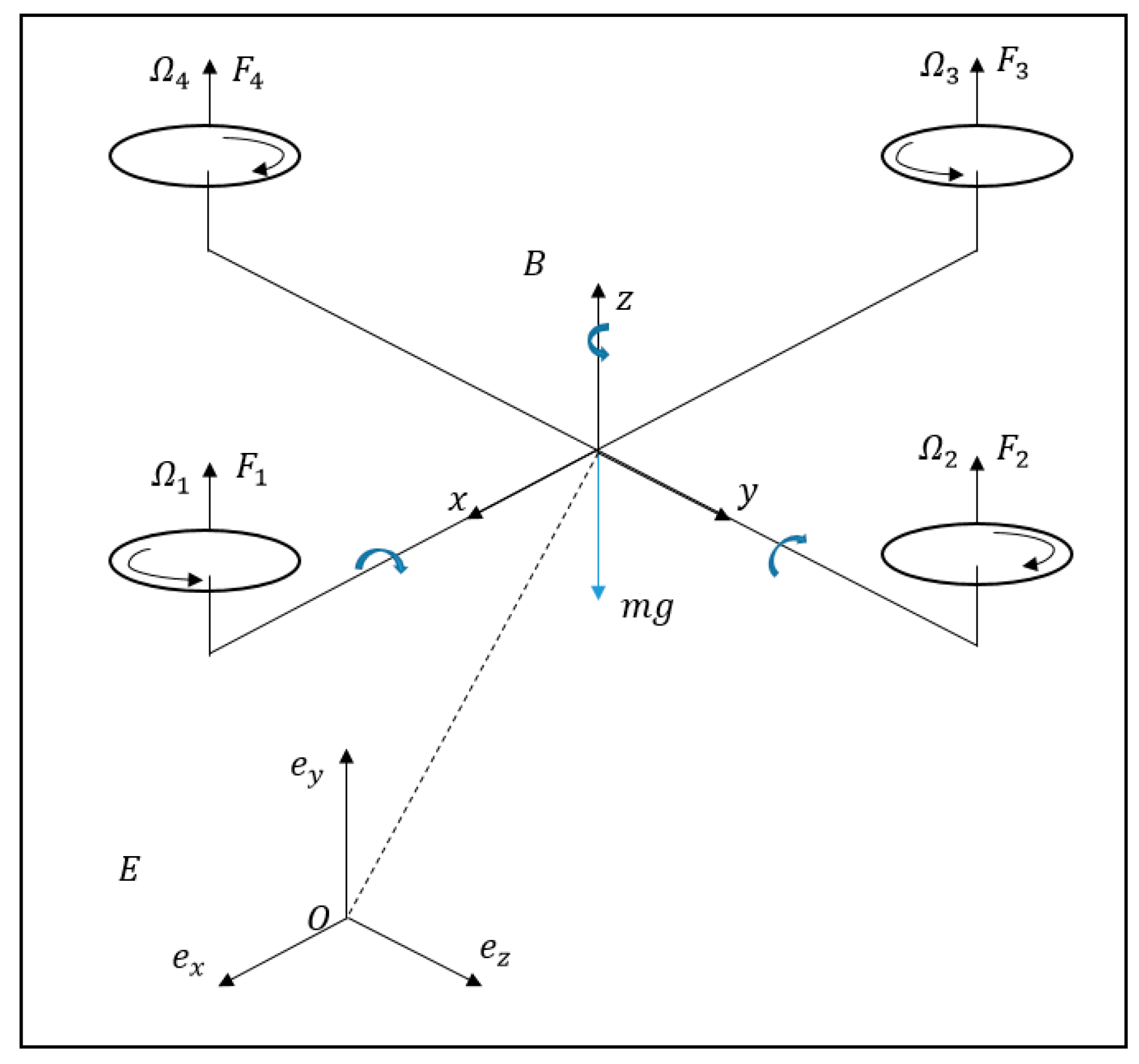
2. Quadcopter Modeling

A quadcopter is subject to torques and forces (Figure 1). Quadcopter dynamics are examined in an earth-fixed coordinate E and an inertial coordinate B. The quadcopter model consists of two counterclockwise and two clockwise rotating motors. The arm length is denoted by L. The quadcopter dynamics can be presented as [15]
{ φ ¨ = ( U φ + ( I y I z ) θ ˙ ψ ˙ J ¯ m θ ˙ Ω K 1 φ ˙ ) / I x θ ¨ = ( U θ + ( I z I x ) φ ˙ ψ ˙ J ¯ m φ ˙ Ω K 2 θ ˙ ) / I y ψ ¨ = ( U ψ + ( I x I y ) φ ˙ θ ˙ K 3 ψ ˙ ) / I z x ¨ = { U T ( cos φ sin θ cos ψ + sin φ sin ψ ) K 4 x ˙ } / m y ¨ = { U T ( cos φ sin θ sin ψ sin φ sin ψ ) K 5 y ˙ } / m z ¨ = g + { U T ( cos φ cos θ ) K 6 z ˙ } / m
where I x , I y , I z are the inertia moments along the x , y , z directions, respectively; K i is drag term, i = 1 . . 6 ; J ¯ m is the inertia moment of an each rotor and Ω = ω 3 + ω 4 ω 1 ω 2 , with ω i being the rotational speed produced by the i th motor; m is the total mass; φ , θ , and ψ are the roll angle, pitch angle, and yaw angle, respectively; and x , y , and z denote three translational movements. The control inputs are described as
{ U T = F 1 + F 2 + F 3 + F 4 U φ = ( F 4 F 2 ) L U θ = ( F 3 F 1 ) L U ψ = τ 1 τ 2 + τ 3 τ 4
where τ i = d ω i 2 and F i = b ω i 2 represent the torque and overall force, respectively, generated by each motor, i = 1 . . 4 and b and d are thrust coefficient and aerodynamic drag coefficient.

3. Methodology

This section will present a robust FD and FTC scheme for the quadcopter under actuator fault. In Section 3.1, the robust FD method is proposed to estimate the magnitude of time-varying actuator fault, which is improved from the normal Thau observer design. A robust attitude controller based on adaptive sliding mode technique is presented in Section 3.2 to handle the uncertainties; partial loss of control effectiveness in actuator (the fault estimation value (Section 3.1), which is is smaller than the threshold value); and chattering problem. In Section 3.3, the proportional–integral–derivative (PID) controller is designed to control three translational movements. We choose the PID controller for translational movements because in a commercial quadcopter the position controller has a lower response than attitude controller. Moreover, when the attitude controller is robust to uncertainties and actuator faults, the performance of position controller will be enhanced as well [27]. The fault-tolerant controller is designed in Section 3.4 to reconfigure the allocation matrix of quadcopter to handle the complete actuator failure (fault estimation value is larger than threshold value).

3.1. Robust Fault Diagnosis using Nonlinear Observer

3.1.1. Fault Diagnosis using Normal Thau Observer Design

By defining u T = [ U φ U θ U ψ U T ] as the control input vector, x T = [ φ θ ψ z φ ˙ θ ˙ ψ ˙ z ˙ ] as the state vector, and y = [ φ θ ψ z φ ˙ θ ˙ ψ ˙ z ˙ ] as the output vector. Using the linearization technique for the z -direction at the hovering point and nonlinear model for the attitude system [28], Equation (1) is rewritten as
{ x ˙ ( t ) = A x ( t ) + δ ( x , u ) + B u ( t ) + E d d ( t ) y = C x ( t ) ,
where E d , d ( t ) are the disturbance matrix and disturbance vector, A = [ 0 4 × 4 I 4 × 4 0 4 × 4 0 4 × 4 ] , B = [ 0 0 0 0 1 / I x 0 0 0 0 0 0 0 0 1 / I y 0 0 0 0 0 0 0 0 1 / I z 0 0 0 0 0 0 0 0 1 / m ] T , C = I 8 × 8 , and δ ( x , u ) = [ 0 0 0 0 h T ( x , u ) g ] T with h ( x , u ) = [ ( θ ˙ ψ ˙ ( I y I z ) J ¯ m θ ˙ Ω ) / I x ( φ ˙ ψ ˙ ( I z I x ) J ¯ m φ ˙ Ω ) / I y φ ˙ θ ˙ ( I x I y ) / I z ] T . Under the actuator fault, (3) becomes
{ x ˙ ( t ) = A x ( t ) + δ ( x , u ) + B u ( t ) + F f ( t ) + E d d ( t ) y = C x ( t ) ,
where F , f ( t ) are the fault matrix and fault vector, respectively, with f ( t ) = [ f 1 f 2 f 3 f 4 ] T .
Remark 1.
The fault matrix is chosen as F = B and the fault vector f ( t ) is the estimate of fault offset of vector u [28]. After the fault vector is achieved, the fault magnitude of each actuator f o i , i = 1 . . 4 is obtained using Equation (2) as
[ f 1 f 2 f 3 f 4 ] = [ 1 1 1 1 0 L 0 L L 0 L 0 d / b d / b d / b d / b ] [ f o 1 f o 2 f o 3 f o 4 ]
In the Thau observer design [28,29], the two following conditions must be met:
C1 the pair ( C , A ) is observable.
C2 the nonlinear function δ ( x , u ) must be continuously differentiable and Lipschitz locally, with a constant γ , i.e., δ ( x 1 ( t ) , u ( t ) ) δ ( x 2 ( t ) , u ( t ) ) γ x 1 x 2 .
The Thau observer based on Equation (4) is described as
{ x ^ ˙ ( t ) = A x ^ ( t ) + B u ( t ) + K ¯ ( y ^ ( t ) y ( t ) ) + δ ( x ^ , u ) y ^ = C x ^ ( t ) ,
where K ¯ is the gain matrix determined by
Lemma 1.
[29] If the given gain matrix K ¯ satisfies
K ¯ = Y 1 C T ,
then matrix Y is achieved from equation
A T Y + Y A C T C + κ C T Y = 0 ,
where κ is a positive parameter such that Y 0 .

3.1.2. Fault Diagnosis Using Adaptive Sliding Mode Thau Observer

Two conditions and lemmas must be met for observer design
C3 f ( t ) and f ˙ ( t ) are norm-bounded, i.e., f ( t ) p 1 , f ˙ ( t ) p 2 , with p 1 , p 2 > 0.
C4 The disturbance is bound d ( t ) S , S is unknown constant.
Lemma 2.
There exit a matrix Y = Y T 0 and constant ρ > 0 , the following inequality holds.
2 x 1 T x 2 1 ρ x 1 T Y x 1 + ρ x 2 T Y 1 x 2 ,
Lemma 3.
There exit a matrix Y 0 , the following condition holds.
2 e T Y ( δ ( x 1 , u ) δ ( x 2 , u ) ) γ 2 e T Y Y e + e T e ,
The adaptive sliding mode Thau observer (ASMTO) has the form
{ x ^ ˙ ( t ) = A x ^ ( t ) + B u ( t ) + δ ( x ^ , u ) + E d v ( t ) + F f ^ ( t ) K ¯ ( y ^ ( t ) y ( t ) ) k ^ H ( y ^ ( t ) y ( t ) ) / 2 y ^ = C x ^ ( t ) ,
where x ^ ( t ) R n is the observer state vector, f ^ ( t ) R l is the estimate of f ( t ) , and y ^ ( t ) R q is the observer output vector, respectively. H is a matrix to be determined, v ( t ) and k ^ are given by
s ˙ ( t ) = α M 1 e y ( t ) v ( t ) = s ( t ) M 1 e y ( t ) M 1 e y ( t ) k ^ ˙ = l k H ( y ^ ( t ) y ( t ) 2 ,
where α and l k are constants and M 1 is discussed below.

3.1.3. Stability Analysis

Define
e x = x ^ ( t ) x ( t ) n ˜ ( t ) = s ( t ) S e k = k ^ k e y = y ^ ( t ) y ( t ) e f = f ^ ( t ) f ( t ) ,
where k is a constant, then the error dynamics can be obtained from Equations (4), (7), and (11) as
e ˙ x ( t ) = ( A K ¯ C ) e x + δ ( x ^ , u ) δ ( x , u )    + F e f + E d ( v ( t ) d ( t ) ) 1 2 k ^ H C e x ,
Theorem 1.
Given observer gain K ¯ , if there exist matrices Y = Y T > 0 , Q = Q T > 0 , M 1 and M 2 can be derived as follows
[ Y ( A K ¯ C ) + ( A K ¯ C ) T Y 0 I 0 1 σ Q 0 I 0 I ] < 0 ,
F T Y = 1 σ M 1 C
E d T Y = 1 σ M 2 C
Y = H C
where σ > 0 is a constant.
Then the fault estimation law is constructed as
f ^ ˙ ( t ) = Λ M 1 e y ,
where Λ is the learning rate matrix Λ = Λ T > 0 .
Proof. 
Choose the Lyapunov function:
V ( t ) = e x T Y e x + 1 σ e f T Λ 1 e f + 1 σ n ˜ T α 1 n ˜ + 1 2 l k 1 e k 2 .
Differentiating V ( t ) is
V ˙ ( t ) = e ˙ x T ( t ) Y e x ( t ) + e x T ( t ) Y e ˙ x ( t ) + 2 σ e f T ( t ) Λ 1 e ˙ f ( t ) + 2 σ s ˙ ( t ) α 1 s ˜ ( t ) + l k 1 e k e ˙ k = e x T ( t ) [ Y ( A K ¯ C ) + ( A K ¯ C ) T Y ] e x ( t ) + 2 e x T ( t ) Y E d ( v ( t ) d ( t ) ) + 2 e x T ( t ) Y F e f ( t ) + 2 e x T ( t ) Y ( δ ( x ^ , u ) δ ( x , u ) ) k ^ e x T Y H C e x + 2 σ e f T Λ 1 f ^ ˙ ( t ) 2 σ e f T Λ 1 f ˙ ( t ) + 2 σ M 1 e y ( t ) ( s ( t ) S ) + e k H C e x 2 ,
Using Theorem 1, we achieve
2 e x T ( t ) Y F e f ( t ) + 2 σ e f T Λ 1 f ^ ˙ ( t ) = 2 e x T ( t ) Y F e f ( t ) + 2 σ e f T Λ 1 ( Λ M 1 e y ) = 0
2 e x T ( t ) Y E d ( v ( t ) d ( t ) ) = 2 σ ( M 2 e y ( t ) ) T ( s ( t ) M 1 e y ( t ) M 1 e y ( t ) d ( t ) ) < 2 σ M 1 e y ( t ) ( s ( t ) S )
From Lemma 2, it is easy to see that
2 σ e f T ( t ) Λ 1 f ˙ ( t ) = 2 σ ( e f T ( t ) ) ( Λ 1 f ˙ ( t ) ) 1 σ ( e f T ( t ) Q e f ( t ) + f ˙ T ( t ) Λ 1 Q 1 Λ 1 f ˙ ( t ) ) 1 σ e f T ( t ) Q e f ( t ) + 1 σ p 2 2 λ max ( Λ 1 Q 1 Λ 1 )
where λ max represents the largest eigenvalue of the corresponding matrix.
From Lemma 3, we obtain
e x T ( t ) [ Y ( A K ¯ C ) + ( A K ¯ C ) T Y ] e x ( t ) + 2 e x T ( t ) Y ( δ ( x ^ , u ) δ ( x , u ) ) e x T ( t ) [ Y ( A K ¯ C ) + ( A K ¯ C ) T Y + I ] e x ( t ) + γ 2 e x T Y Y e x ,
With Equations (22)–(25), and k = γ 2 > 0 , (21) becomes
V ˙ ( t ) e x T ( t ) [ Y ( A K ¯ C ) + ( A K ¯ C ) T Y + I ] e x ( t ) + k e x T Y Y e x k ^ e x T Y H C e x + e k H C e x 2 + 1 σ e f T ( t ) Q e f ( t ) + 1 σ p 2 2 λ max ( Λ 1 Q 1 Λ 1 ) ,
From Equations (18) and (26), we achieve
V ˙ ( t ) e x T ( t ) [ Y ( A K ¯ C ) + ( A K ¯ C ) T Y + I ] e x ( t ) ( k ^ k ) H C e x 2 + e k H C e x 2 + 1 σ e f T ( t ) Q e f ( t ) + 1 σ p 2 2 λ max ( Λ 1 Q 1 Λ 1 ) ) e x T ( t ) [ Y ( A K ¯ C ) + ( A K ¯ C ) T Y + I ] e x ( t ) + 1 σ e f T Q e f + η ξ T ( t ) Φ ξ ( t ) + η ,
where η = p 2 2 λ max ( Λ 1 Q 1 Λ 1 ) σ , ξ ( t ) = [ e x T ( t ) e f T ( t ) ] , and Ξ = [ Y ( A K ¯ C ) + ( A K ¯ C ) T Y + I 0 0 1 σ Q ]
If Ξ < 0 , then V ˙ ( t ) < 0 for σ ξ ( t ) 2 > η , where σ = λ min ( Ξ ) . This completes the proof according to Lyapunov theory [25]. ☐
Remark 2.
To solve Equations (15)–(18) simultaneously, we can modify Equations (16)–(18) as [25]
[ η 1 I F T Y 1 σ M 1 C ( F T Y 1 σ M 1 C ) T η 1 I ] > 0 ,
[ η 2 I E d T Y 1 σ M 2 C ( E d T Y 1 σ M 2 C ) T η 2 I ] > 0
[ η 3 I Y H C ( Y H C ) T η 3 I ] > 0
Four indicators d i are defined to recognize the fault-free and faulty (total loss of effectiveness in one motor) operation through Equations (5) and (19) as
d i = { 0 , f o i < d T   fault - free   operation   no   fault 1 , f o i > d T   faulty   operation   fault
where d T is a predefined threshold.

3.2. Attitude Controller

3.2.1. Modeling of Quadcopter in Faulty Operation

Under faulty operation, Equation (1) can be rewritten as
{ φ ¨ = ( U ¯ φ + ( I y I z ) θ ˙ ψ ˙ J ¯ m θ ˙ Ω K 1 φ ˙ ) / I x θ ¨ = ( U ¯ θ + ( I z I x ) φ ˙ ψ ˙ J ¯ m φ ˙ Ω K 2 θ ˙ ) / I y ψ ¨ = ( U ¯ ψ + ( I x I y ) φ ˙ θ ˙ K 3 ψ ˙ ) / I z x ¨ = { U ¯ T ( cos φ sin θ cos ψ + sin φ sin ψ ) K 4 x ˙ } / m y ¨ = { U ¯ T ( cos φ sin θ sin ψ sin φ sin ψ ) K 5 y ˙ } / m z ¨ = g + { U T ( cos φ cos θ ) K 6 z ˙ } / m
where U ¯ φ , U ¯ θ , U ¯ ψ , U ¯ T are the control inputs for faulty operation denoted by
{ U ¯ T = F ˜ 1 + F ˜ 2 + F ˜ 3 + F ˜ 4 U ¯ φ = L ( F ˜ 4 F ˜ 2 ) U ¯ θ = L ( F ˜ 3 F ˜ 1 ) U ¯ ψ = d ( F ˜ 1 F ˜ 2 + F ˜ 3 F ˜ 4 ) / b
The actuator fault model can be written as
F ˜ i = ( 1 ϑ ¯ i ) F i
where 0 < ϑ ¯ i < 1   ( i = 1 . . 4 ) denotes the partial loss of control effectiveness in the i th actuator: a value of ϑ ¯ i = 0 implies that no fault is present in the i t h actuator, while ϑ ¯ i = 1 implies a total loss of effectiveness.
From Equations (32)–(34), we obtain
{ φ ¨ = ( U φ + ( I y I z ) θ ˙ ψ ˙ J ¯ m θ ˙ Ω K 1 φ ˙ ) / I x + d 1 θ ¨ = ( U θ + ( I z I x ) φ ˙ ψ ˙ J ¯ m φ ˙ Ω K 2 θ ˙ ) / I y + d 2 ψ ¨ = ( U ψ + ( I x I y ) φ ˙ θ ˙ K 3 ψ ˙ ) / I z + d 3 x ¨ = { U T ( cos φ sin θ cos ψ + sin φ sin ψ ) K 4 x ˙ } / m + d 4 y ¨ = { U T ( cos φ sin θ sin ψ sin φ sin ψ ) K 5 y ˙ } / m + d 5 z ¨ = g + { U T ( cos φ cos θ ) K 6 z ˙ } / m + d 6
where the model uncertainties are given by
{ d 1 = L ( ϑ ¯ 4 F 4 ϑ ¯ 2 F 2 ) / I x d 2 = L ( ϑ ¯ 3 F 3 ϑ ¯ 1 F 1 ) / I y d 3 = d ( ϑ ¯ 1 F 1 ϑ ¯ 2 F 2 + ϑ ¯ 3 F 3 ϑ ¯ 4 F 4 ) / b I z d 4 = ( cos ϕ sin θ cos ψ + sin ϕ sin ψ ) ( ϑ ¯ 1 F 1 + ϑ ¯ 2 F 2 + ϑ ¯ 3 F 3 + ϑ ¯ 4 F 4 ) / m d 5 = ( cos ϕ sin θ sin ψ sin ϕ sin ψ ) ( ϑ ¯ 1 F 1 + ϑ ¯ 2 F 2 + ϑ ¯ 3 F 3 + ϑ ¯ 4 F 4 ) / m d 6 = cos ϕ cos θ ( ϑ ¯ 1 F 1 + ϑ ¯ 2 F 2 + ϑ ¯ 3 F 3 + ϑ ¯ 4 F 4 ) / m

3.2.2. Adaptive Sliding Mode Control for Attitude System

By defining x ¯ = [ φ φ ˙ θ θ ˙ ψ ψ ˙ ] T = [ x ¯ 1 x ¯ 2 x ¯ 3 x ¯ 4 x ¯ 5 x ¯ 6 ] T as the state vector and U = [ U ϕ U θ U ψ ] = [ u 1 u 2 u 3 ] as the control inputs, the rotational movement equations of the quadcopter become:
Roll control system:
{ x ¯ ˙ 1 = x ¯ 2 x ¯ ˙ 2 = f 1 ( x ¯ ) + g 1 u 1 ( t ) + ξ 1 ( x ¯ , t ) + ζ 1
where ξ 1 ( x ¯ , t ) = ( I y I z ) / ( I x ) ( x ¯ 4 x ¯ 6 ) J ¯ m x ¯ 4 Ω ; f 1 ( x ¯ ) = d 1 ; g 1 = 1 / I x ; ζ 1 = K 1 x ¯ 2 is the disturbance;
Pitch control system:
{ x ¯ ˙ 3 = x ¯ 4 x ¯ ˙ 4 = f 2 ( x ¯ ) + g 2 u 2 ( t ) + ξ 2 ( x ¯ , t ) + ζ 2
where ξ 2 ( x ¯ , t ) = ( I z I x ) / ( I y ) ( x ¯ 2 x ¯ 6 ) J ¯ m x ¯ 2 Ω ; f 2 ( x ¯ ) = d 2 ; g 3 = 1 / I y ; ζ 2 = K 2 x ¯ 4 is the disturbance;
Yaw control system:
{ x ¯ ˙ 5 = x ¯ 6 x ¯ ˙ 6 = f 3 ( x ¯ ) + g 3 u 3 ( t ) + ξ 3 ( x ¯ , t ) + ζ 3
where ξ 3 ( x ¯ , t ) = ( I x I y ) / ( I z ) ( x ¯ 2 x ¯ 4 ) ; f 3 ( x ¯ ) = d 3 ; g 3 = 1 / I z ; ζ 3 = K 3 x ¯ 6 is the disturbance;
Generally, rotational movement equations can be derived as
{ x ¯ ˙ 2 i 1 = x ¯ 2 i x ¯ ˙ 2 i = f i ( x ¯ ) + g i u i ( t ) + ξ i ( x ¯ , t ) + ζ i
The function f i ( x ¯ ) is approximated using radius basis function (RBF) neural network as [30]
D k = exp ( x ¯ b k 2 2 σ k 2 ) ,
f i ( x ¯ ) = W ¯ f i T D f i ( x ¯ ) + ε ¯ f i ,
where x = [ e i e ˙ i ] is the state input; k the number of hidden nodes; D f i is the output of Gaussian function; W ¯ f i T is the approximation weight; and ε ¯ f i is the approximation error assumed to be bounded by | ε ¯ f i | ε f i * , in which ε f i * > 0 is a small positive constant.
The desired attitude is defined as x ¯ i d . The main goal is to choose a control law, u i , such that x ¯ 2 i 1 ( t ) x ¯ i d as t , with i = 1 . . 3 . If the control error is defined as
e i = x ¯ 2 i 1 x ¯ i d
the sliding surface is chosen as
s i = e ˙ i + c i e i + v i e i
where c i , v i are the positive constants.
From Equations (43) and (44), s ˙ i is written as
s ˙ i = f i ( x ¯ ) + g i u i ( t ) + ζ i + ξ i ( x ¯ , t ) x ¯ ¨ i d + c i e ˙ i + v i e i
The control law is chosen as
u i = ( ξ i ( x ¯ , t ) c i e ˙ i v i e i + x ¯ ¨ i d W ¯ ^ f i T D f i ( x ) Γ ^ i s i g n ( s i ) ) g i
and updated by
Γ ^ ˙ i = α i 1 | s i |
W ¯ ^ ˙ f i = α i 2 s i D f i
where s i g n ( . ) is the sign function and α i 1 and α i 2 are positive constants.
Theorem 2.
If the sliding surface is designed as Equation (44) and the control law is chosen as Equation (46), then the system in Equation (32) is stable and control errors are forced to zero.
Proof. 
The Lyapunov function is chosen as
V = 1 2 s i 2 + 1 2 Γ ˜ i 2 α i 1 + 1 2 W ˜ f i T W ˜ f i α i 2
where W ˜ f i = W ¯ f i W ¯ ^ f i , Γ ˜ i = Γ i Γ ^ i ; Γ ^ i , W ¯ ^ f i are the estimates of Γ i and W ¯ f i , respectively.
Differentiating V yields
V ˙ = s i s ˙ i Γ ˜ i Γ ^ ˙ i α i 1 W ˜ f i T W ¯ ^ ˙ f i α i 2 = s i ( f i ( x ¯ ) W ¯ f i T V f i ( x ) ) | s i | Γ i + s i ζ i = s i ε ¯ f i + s i ζ i | s i | Γ i | s i | ( | ε ¯ i + ζ i | Γ i )
 ☐
Assumption 1.
The disturbance ζ i is bounded by | ζ i | ζ d , where ζ d > 0 is unknown parameter. There exists the positive parameter Γ i , such that | ζ i ( x ¯ , t ) + ε ¯ i | | ζ i ( x ¯ , t ) | + | ε ¯ i | ζ d + ε f i * = Γ i .
It is clear from the Assumption 1 that V ˙ 0 . If s i = 0 , from Equation (44), one can achieve
lim t s i = lim t ( e ˙ i + c i e i + v i e i ) = lim t { ( x ¯ ˙ 2 i 1 x ¯ ˙ i d ) + c i ( x ¯ 2 i 1 x ¯ i d ) + v i ( x ¯ 2 i 1 x ¯ i d ) }
Because c i and v i are positive constants, Equation (51) can be expressed as
lim t ( x ¯ ˙ 2 i 1 x ¯ ˙ i d ) = 0 , lim t ( x ¯ 2 i 1 x ¯ i d ) = 0
Remark 3.
To avoid the chattering issue, the s i g n function is replaced by a saturation function as
s a t ( s i ) = { s i if   | s i | 1 s i g n ( s i ) if   | s i | > 1 , i = 1 , 2 , 3

3.3. Position Controller

A PID controller was used to control the position of the quadcopter UAVs as follows
R ¨ = R ¨ d + K d ( R ˙ R ˙ d ) + K p ( R R d ) + K i ( R R d ) d t
where R d = [ X d , Y d , Z d ] T is the desired position, R = [ X , Y , Z ] T is the actual position, and K p , K i , and K d are the positive diagonal matrices.
The total thrust, desired roll angle, and desired pitch angle are described as
U T = m X ¨ 2 + Y ¨ 2 + ( Z ¨ g ) 2 φ d = sin 1 ( m X ¨ sin ( ψ ) m Y ¨ cos ( ψ ) ) / U T θ d = cos 1 ( m Z ¨ m g ) / ( U T cos ( φ ) )

3.4. Fault-Tolerant Controller

Once the fault diagnosis unit realizes that one of the rotors is experiencing a fault, it needs to modify the control scheme to reduce its effect. This control strategy aims to enable the quadcopter to land safely. In a faulty operation (complete loss of effectiveness in one rotor) Equation (2) is modified to change the rotor’s thrust force F i . This is achieved through an algorithm to reconfigure the controller in the presence of a fault (Figure 2). When a fault occurs, the goal of this FTC approach is to land horizontally ( φ = 0 and θ = 0 ) and to sacrifice the yaw control. The difference between the faulty and fault-free operations is that in the faulty operation the faulty rotor no longer contributes to the control of roll and pitch angles but only of elevation. Assuming rotor 2, the control allocation is obtained from Equation (2) as
[ U T U φ U θ ] = [ 1 1 1 0 0 L L L 0 ] [ F 1 F 3 F 4 ]

4. Simulation Results

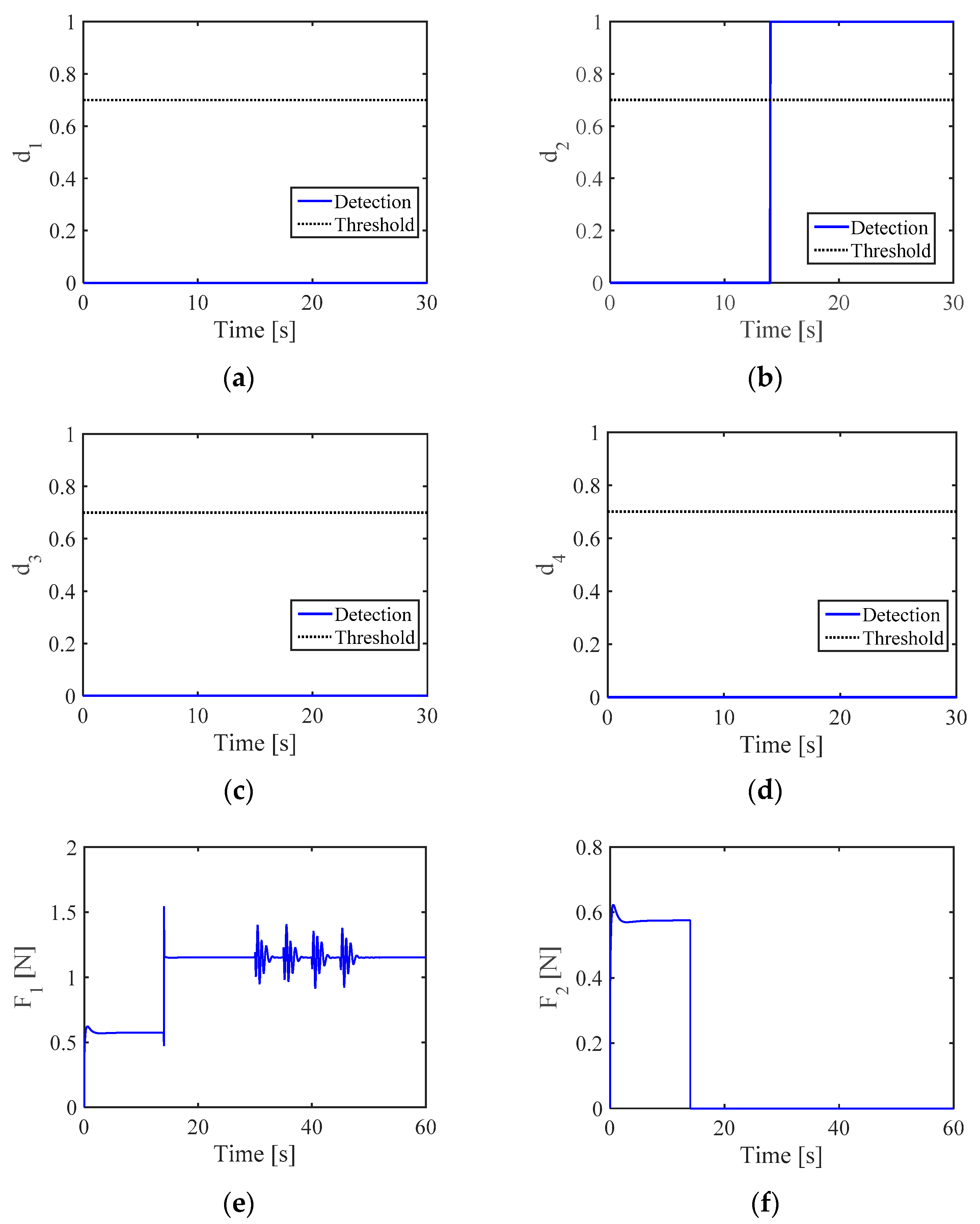
4.1. Fault Diagnosis Results

For simplicity, the altitude and attitude control are tested in this section. The quadcopter parameters in paper [27] are used for this paper. The conditions C1 and C2 are easy to obtain. The learning rate and sampling time are chosen as Γ = d i a g ( 4 , 4 , 4 , 4 ) and T = 0.001 s , respectively. The matrices are designed for ASMTO as
F = B , Q = 100 × I 8 × 8 , E d = [ 1 1 1 1 1 1 1 1 ] T ,
M 1 = [ 127.62 127.62 127.62 127.62 0.87 0.87 0.87 0.87 ] ,
M 2 = [ 117 0 0 0 17008 0 0 0 0 117 0 0 0 17014 0 0 0 0 67 0 0 0 9817 0 0 0 0 4 0 0 0 555 ] , K = [ 200 0 0 1 0 0 0 200 0 0 1 0 0 0 200 0 0 1 1 0 0 200 0 0 0 1 0 0 200 0 0 0 1 0 0 200 ] ,
Y = [ 127.62 0 0 0 0.87 0 0 0 0 127.62 0 0 0 0.87 0 0 0 0 127.62 0 0 0 0.87 0 0 0 0 127.62 0 0 0 0.87 0.87 0 0 0 127.62 0 0 0 0 0.87 0 0 0 127.62 0 0 0 0 0.87 0 0 0 127.62 0 0 0 0 0.87 0 0 0 127.62 ] .
The performance of the altitude and attitude control is shown in Figure 3, while the relationship between inputs and motor outputs is given by Equation (2).
To test the performance of fault estimation shown in Equation (19), a fault is created in motors 1 and 2 as follows
ω 1 2 = { 0 ,          t < 14 150 2 ,     t 14
ω 2 2 = { 0 ,            t < 14 ( 170 sin ( 2 π t / 25 ) ) 2 ,     t 14
The results indicate that the estimation value converges almost immediately to the fault offset value (Figure 4). Figure 5, Figure 6 and Figure 7 show the interplay between the attitude angles, control inputs, and forces. Attitude angles are capable of maintaining their states while the altitude and control inputs change once a fault occurs at t = 14 s (Figure 5 and Figure 6).

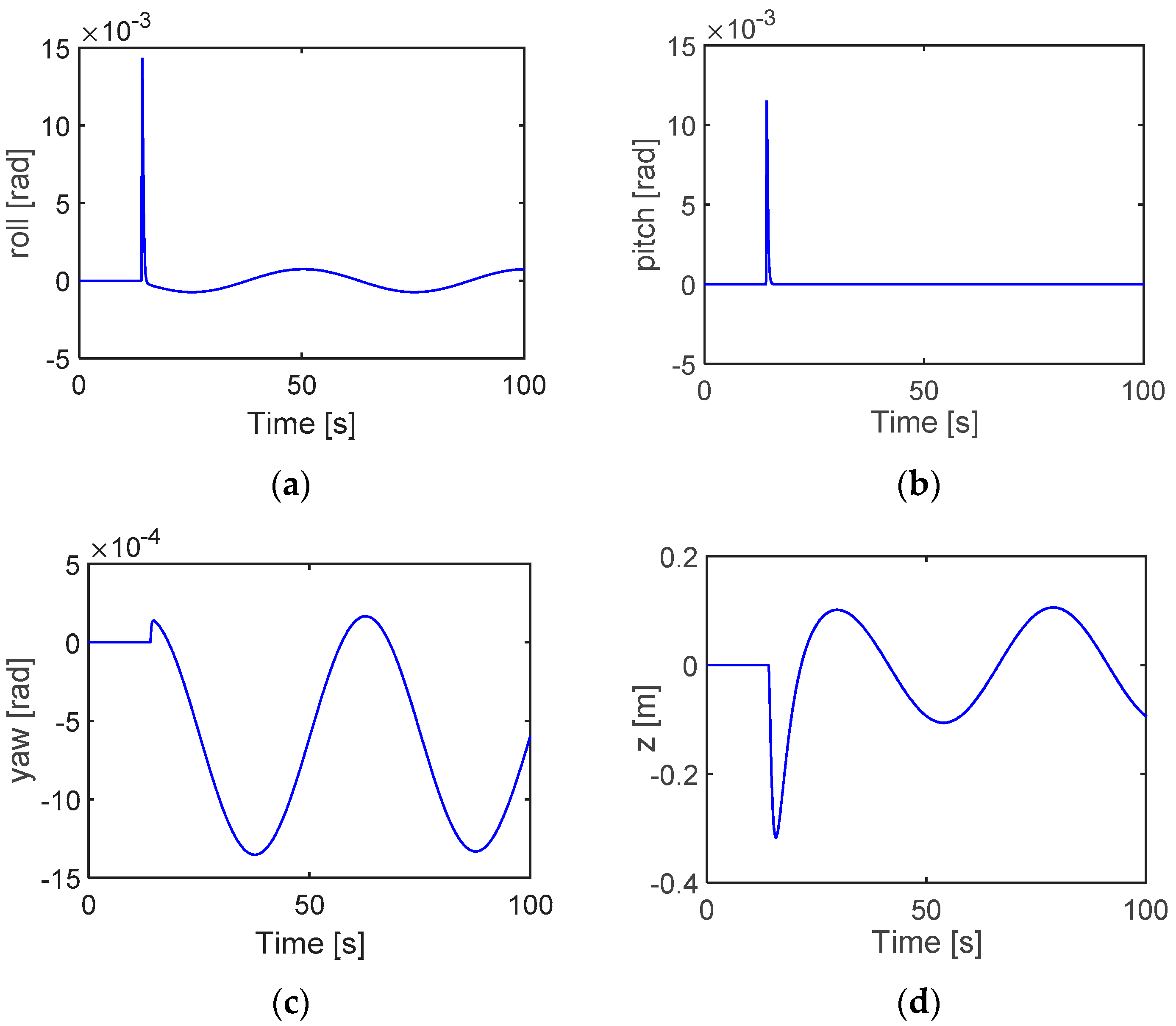
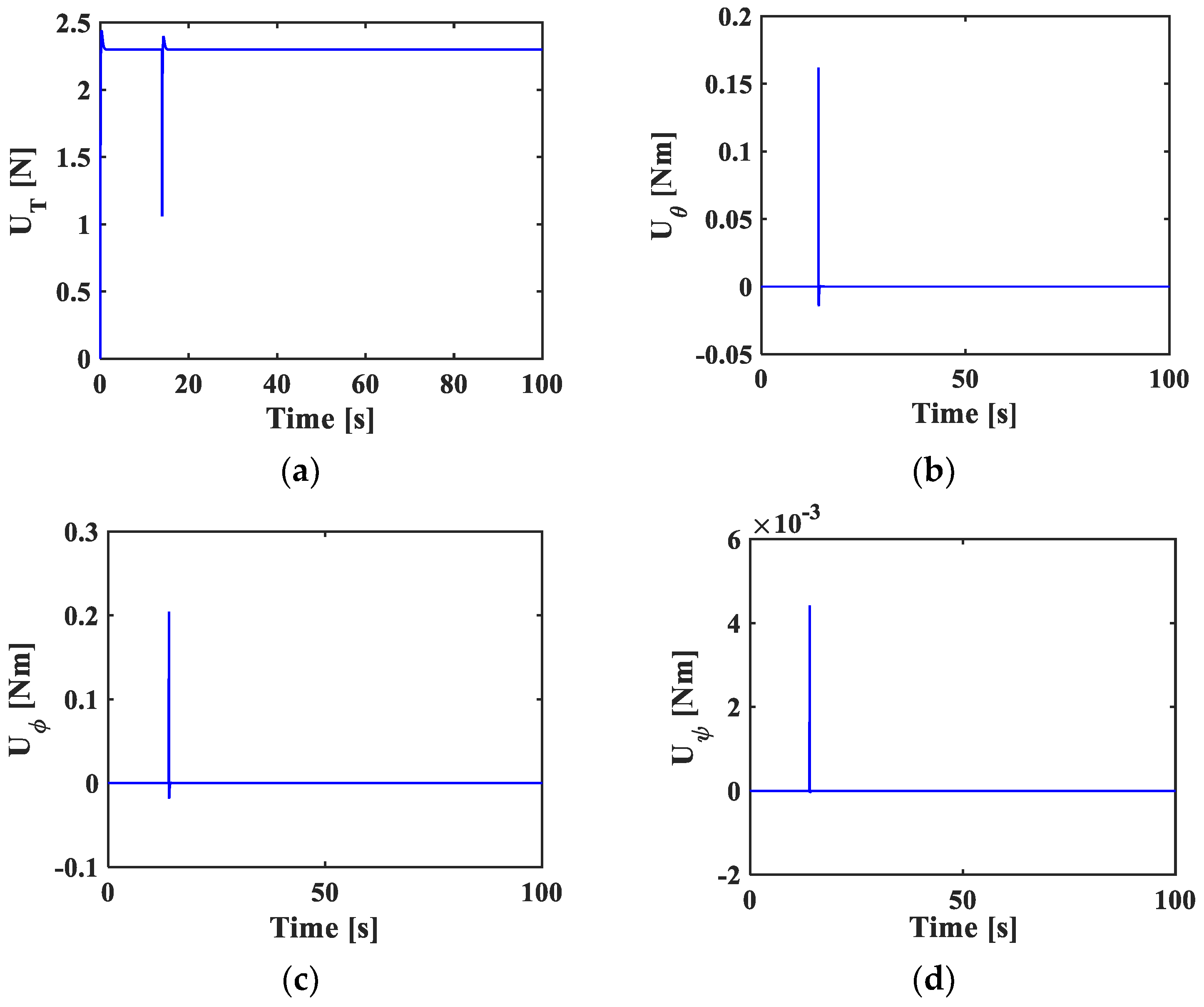
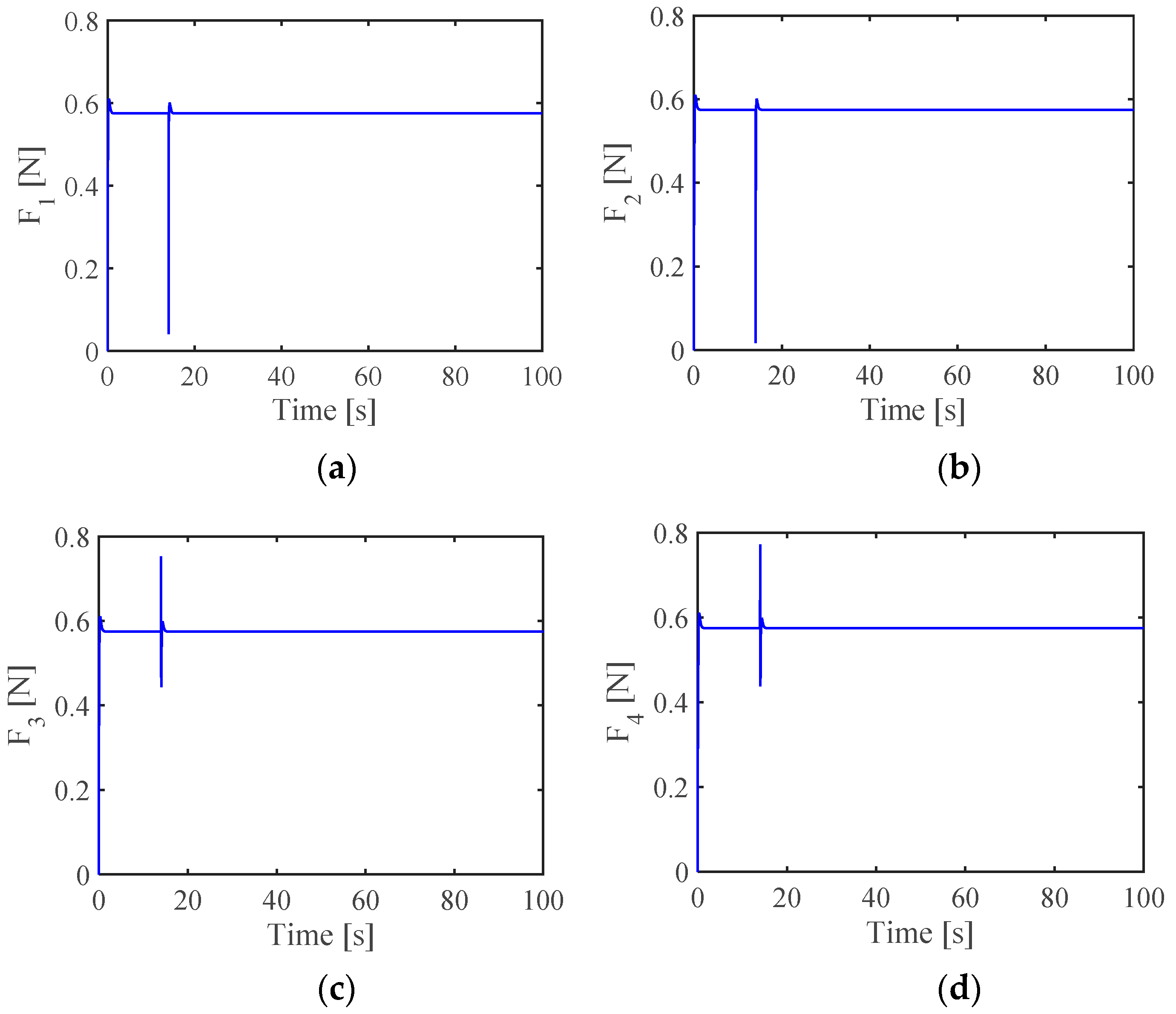
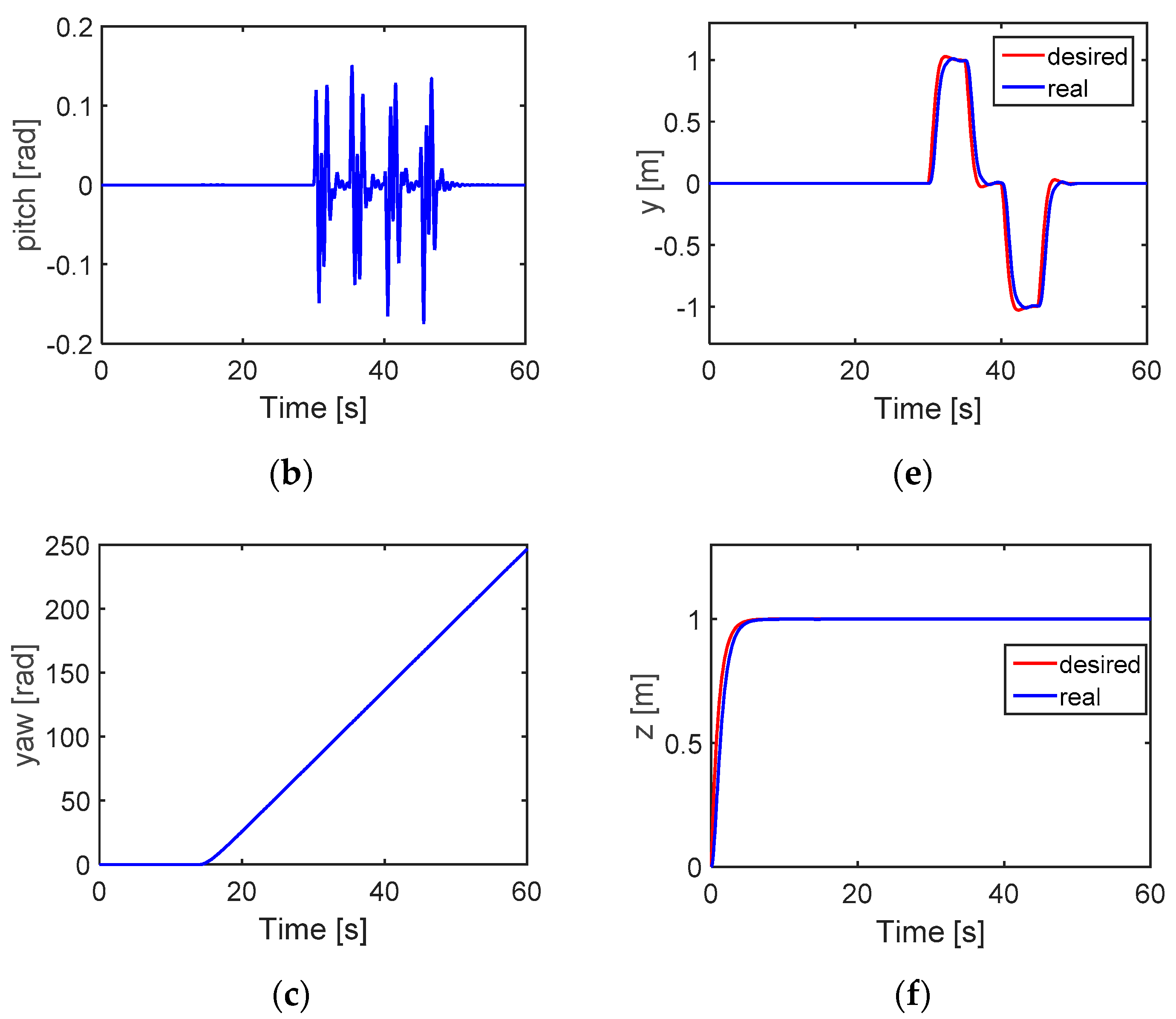
4.2. Fault-Tolerant Control Results

Two scenarios are illustrated to show the response of our fault-tolerant controller with the complete loss actuator. In the first scenario (Scenario 1), the quadcopter, once the fault has occurred, is only supposed to reach a desired altitude of 1 m with all other variables set to zero. In the second scenario (Scenario 2), the quadcopter is required to track a specific trajectory after a fault has occurred. For both scenarios, the fault (total loss of effectiveness) occurs in rotor 2. The attitude angles and position angles in Scenario 1 start to deviate from the command after the fault occurs at t = 14 s (Figure 8). While the quadcopter recovers the desired altitude after ~ 1 s , the yaw angle, ψ , increases gradually as control over ψ has been sacrificed in the fault-tolerant controller. Because the FD method can estimate fault magnitude quickly, the fault-tolerant controller is started quickly for fault compensation, which can reduce the oscillation for rotation and translation movement (Figure 8). Angular rates and linear velocities stabilize within a few seconds (Figure 9). Interestingly, the yaw rate converges to a constant value. Once the fault in rotor 2 is detected, the force in rotor 4 is decreased to balance the moment of roll, while the forces in rotors 1 and 3 are increased to compensate the loss in thrust (Figure 10a). It should be noted that when fault magnitude exceeds a certain threshold ( d T = 0.7 ) shown in (30), the fault-tolerant controller is activated (Figure 10b).
In Scenario 2, the fault-tolerant controller is capable of delivering a good tracking response, both in the horizontal and vertical directions and despite the actuator fault (Figure 11). Once again, the yaw rate converges to a steady state (Figure 12) and control over the yaw angle is sacrificed once the fault-tolerant controller has been activated (Figure 13a). The corresponding torques (Figure 13b) indicate that once the fault occurs, the force in rotor 4 is decreased to compensate the moment of roll, while the forces in rotors 1 and 3 are increased to compensate for the loss in thrust.
Remark 4. In the total loss effectiveness of the actuator, the convergence rate of attitude system (roll and pitch) depends on the fault diagnosis scheme and adaptive sliding mode control method presented in Section 3. This mean that if the fault estimation algorithm or parameter gains of adaptive sliding mode control is slow, the system will oscillate more, which will affect the energy of system. Therefore, we need to consider this problem to save the energy of battery in real flight tests.

5. Conclusions

This paper presented an active FTC scheme for a quadcopter UAV in the presence of a fault leading to the complete loss of the actuator. Robust FD has been used to estimate the time-varying and constant fault under disturbances. We propose a FTC method based on an adaptive SMC scheme both for fault-free and faulty operation. The fault-tolerant controller is activated once the fault magnitude exceeds a certain threshold. Using simulations, we examined two scenarios to verify the fault-tolerant controller. The simulation results showed that the quadcopter can hover a certain altitude and deliver a good tracking performance despite a complete loss of actuator effectiveness. In future works, we plan to validate the model of quadcopter before implementing fault-tolerant control method on onboard controller for experimental tests, which will help us to validate the algorithm and determine how the method can handle multiple faults.

Author Contributions

Conceptualization, N.P.N. and S.K.H.; Methodology, N.P.N.; Software, N.P.N.; Validation, N.P.N.; Formal Analysis, N.P.N.; Investigation, N.P.N.; Resources, N.P.N.; Data Curation, N.P.N.; Writing-Original Draft Preparation, N.P.N.; Writing-Review & Editing, S.K.H.; Visualization, N.P.N.; Supervision, S.K.H.; Project Administration, S.K.H.; Funding Acquisition, S.K.H.

Funding

This research received no external funding.

Acknowledgments

This research was supported by the MSIT (Ministry of Science and ICT), Korea, under the ITRC (Information Technology Research Center) support program (IITP-2019-2018-0-01423) supervised by the IITP (Institute for Information & communications Technology Promotion). The authors gratefully acknowledge the helpful comments and suggestions of the reviewers which have improved the presentation.

Conflicts of Interest

The authors declare no conflict of interest.

References

  1. Tayebi, A.; MaGilvray, S. Attitude stabilization of a VTOL quadrotor aircraft. IEEE Trans. Control Syst. Technol. 2006, 14, 562–571. [Google Scholar] [CrossRef] [Green Version]
  2. Birk, A.; Wiggerich, B.; Bulow, H.; Pfingsthorn, M.; Schwertfeger, S. Safety, Security, and Rescue missions with an Unmanned Aerial Vehicle (UAV). J. Intell. Robot. Syst. 2011, 64, 57–76. [Google Scholar] [CrossRef]
  3. Erdos, D.; Erdos, A.; Watkins, S.E. An experimental UAV system for search and rescue challenge. IEEE Aerosp. Electron. Syst. Mag. 2013, 28, 32–37. [Google Scholar] [CrossRef]
  4. Le, T.; Son, L.H.; Vo, M.T.; Lee, M.Y.; Baik, S.W. A cluster-based boosting algorithm for bankruptcy prediction in a highly imbalanced dataset. Symmetry 2018, 10, 250. [Google Scholar] [CrossRef]
  5. Le, T.; Lee, M.Y.; Park, J.R.; Baik, S.W. Oversampling techniques for bankruptcy prediction: novel features from a transaction dataset. Symmetry 2018, 10, 79. [Google Scholar] [CrossRef]
  6. Nagai, M.; Chen, T.; Shibasaki, R.; Kumagai, H.; Ahmed, A. UAV-Borne 3-D Mapping System by Multisensor Integration. IEEE Trans. Geosci. Remote Sens. 2009, 47, 701–708. [Google Scholar] [CrossRef] [Green Version]
  7. Nex, F.; Remondino, F. UAV for 3D mapping applications: Review. Appl. Geomat. 2014, 6, 1–15. [Google Scholar] [CrossRef]
  8. Lippitt, C.D.; Zhang, S. The impact of small unmanned airborne platforms on passive optical remote sensing: A conceptual perspective. Int. J. Remote Sens. 2018, 39, 4852–4868. [Google Scholar] [CrossRef]
  9. Sharifi, F.; Mirzaei, M.; Gordon, B.W.; Zhang, Y. Fault tolerant control of a quadrotor UAV using sliding mode control. In Proceedings of the Conference on Control and Fault Tolerant Systems, Nice, France, 6–8 October 2010. [Google Scholar]
  10. Li, T.; Zhang, Y.; Gordon, B.W. Nonlinear Fault-Tolerant Control of a quadrotor UAV based on sliding mode control technique. In Proceedings of the 8th IFAC Symposium on Fault Detection, Supervision and Safety of Technical Processes (SAFEPROCESS), Mexico City, Mexico, 29–31 August 2012. [Google Scholar]
  11. Freddi, A.; Lanzon, A.; Longhi, S. A feedback linearization approach to fault tolerance in quadrotor vehicles. In Proceedings of the 18th World Congress the International Federation of Automatic Control, Milano, Italy, 28 August–2 September 2011. [Google Scholar]
  12. Ghandour, J.; Aberkane, S.; Ponsart, J.-C. Feedback linearization approach for standard and fault tolerant control: Application to a quadrotor UAV testbed. J. Phys. Conf. Ser. 2014, 570, 082003. [Google Scholar] [CrossRef]
  13. Hu, Q.; Xiao, B. Adaptive fault tolerant control using integral sliding mode strategy with application to flexible spacecraft. Int. J. Syst. Sci. 2013, 44, 2273–2286. [Google Scholar] [CrossRef]
  14. Wang, B.; Zhang, Y.M. Adaptive sliding mode fault-tolerant control for an unmanned aerial vehicle. Unmanned Syst. 2017, 5, 209–221. [Google Scholar] [CrossRef]
  15. Zhang, Y.; Chamseddine, A. Fault tolerant flight control techniques with application to a quadrotor UAV testbed. In Automatic Flight Control Systems—Latest Developments; Editor, T., Lombaerts, Eds.; Intech: London, UK, 2012; Volume 5, pp. 119–150. [Google Scholar]
  16. Merheb, A.-R.; Noura, H.; Bateman, F. Active fault tolerant control of quadrotor UAV using sliding mode control. In Proceedings of the International Conference on Unmanned Aircraft systems, Orland, FL, USA, 27–30 May 2014. [Google Scholar]
  17. Li, T.; Zhang, Y.; Gordon, B.W. Passive and active nonlinear fault-tolerant control of a quadrotor unmanned aerial vehicle based on the sliding mode control technique. Proc. Inst. Mech. Eng. Part I J. Syst. Control Eng. 2013, 227, 12–23. [Google Scholar] [CrossRef]
  18. Cieslak, J.; Henry, D.; Zolghadri, A. Development of an active fault-tolerant flight control strategy. J. Guid. Control Dyn. 2008, 31, 135–147. [Google Scholar] [CrossRef]
  19. Qi, X.; Qi, J.; Theilliol, D.; Zhang, Y.; Han, J.; Song, D.; Hua, C. A review on fault diagnosis and fault tolerant control methods for single-rotor aerial vehicle. J. Intell. Robot. Syst. 2014, 73, 535–555. [Google Scholar] [CrossRef]
  20. Zhang, Y.; Jiang, J. Integrated active fault-tolerant control using IMM approach. IEEE Trans. Aerosp. Electron. Syst. 2001, 37, 1221–1235. [Google Scholar] [CrossRef]
  21. Lanzon, A.; Freddi, A.; Longhi, S. Flight control of quadrotor vehicle subsequent to a rotor failure. J. Guid. Control Dyn. 2014, 37, 580–591. [Google Scholar] [CrossRef]
  22. Mueller, M.W.; Andrea, R.D. Stability and control of a quadrocopter despite the complete loss of one, two, or three propellers. In Proceedings of the IEEE International Conference on Robotics and Automation, Hong Kong, China, 31 May–7 June 2014. [Google Scholar]
  23. Lippiello, V.; Ruggiero, F.; Serra, D. Emergency landing for a quadrotor in case of a propeller failure: A backstepping approach. In Proceedings of the IEEE/RSJ International Conference on Intelligent Robots and Systems, Chicago, IL, USA, 14–18 September 2014. [Google Scholar]
  24. Merheb, A.-R.; Noura, H.; Bateman, F. Emergency control of AR Drone Quadrotor UAV suffering a total loss of one rotor. IEEE/ASME Trans. Mechatron. 2017, 22, 961–971. [Google Scholar] [CrossRef]
  25. Nguyen, N.P.; Hong, S.K. Sliding mode Thau observer for actuator fault diagnosis of quadcopter UAVs. Appl. Sci. 2018, 8, 1893. [Google Scholar] [CrossRef]
  26. Nguyen, N.P.; Hong, S.K. Robust fault diagnosis for a quadrotor with actuator fault. Int. J. Eng. Technol. 2018, 70, 74–77. [Google Scholar]
  27. Nguyen, N.P.; Hong, S.K. Fault-tolerant control of quadcopter UAVs using robust adaptive sliding mode approach. Energies 2018, 12, 95. [Google Scholar] [CrossRef]
  28. Cen, Z.; Noura, H.; Younes, Y.A. Systematic fault tolerant control based on adaptive Thau observer estimation for quadrotor UAVs. Int. J. Appl. Math. Comput. Sci. 2015, 25, 159–174. [Google Scholar] [CrossRef]
  29. Freddi, A.; Longhi, S.; Monteriù, A. A model-based fault diagnosis system for a mini-quadrotor. In Proceedings of the 7th Workshop on Advanced Control and Diagnosis, Zielona Gora, Poland, 19–20 November 2009. [Google Scholar]
  30. Wang, Z.; Shen, Y.; Zhang, X. Actuator fault estimation for a class of nonlinear descriptor systems. Int. J. Syst. Sci. 2014, 45, 487–496. [Google Scholar] [CrossRef]
Figure 1. Quadcopter configuration.
Energies 12 01139 g001
Figure 2. Fault-tolerant control scheme.
Energies 12 01139 g002
Figure 3. Trajectory performance in fault-free case: (a) Roll angle, (b) Pitch angle, (c) Yaw angle, (d) and z-direction.
Energies 12 01139 g003
Figure 4. Fault estimation in the presence of white noise: (a) F 1 fault offset and (b) F 2 fault offset.
Energies 12 01139 g004
Figure 5. System states in the presence of faults: (a) Roll angle, (b) Pitch angle, (c) Yaw angle, and (d) z-direction.
Energies 12 01139 g005
Figure 6. Controller inputs: (a) Thrust, (b) Roll moment, (c) Pitch moment, and (d) Yaw moment.
Energies 12 01139 g006
Figure 7. Forces for each of the four motors: (a) motor 1′s force, (b) motor 2′s force, (c) motor 3′s force, and (d) motor 4′s force.
Energies 12 01139 g007
Figure 8. Attitude angles and position response for scenario 1: (a) Roll angle, (b) Pitch angle, (c) Yaw angle, (d) x-direction, (e) y-direction, and (f) z-direction.
Energies 12 01139 g008
Figure 9. Angular rates and linear velocities for scenario 1: (a) Roll rate, (b) Pitch rate, (c) Yaw rate, (d) velocity of x-direction, (e) velocity of y-direction, and (f) velocity of z-direction.
Energies 12 01139 g009aEnergies 12 01139 g009b
Figure 10. Forces and detection units for scenario 1: (a) motor 1′s force, (b) motor 2′s force, (c) motor 3′s force, (d) motor 4′s force, (e) fault detection of motor 1, (f) fault detection of motor 2, (g) fault detection of motor 3, and (h) fault detection of motor 4.
Energies 12 01139 g010aEnergies 12 01139 g010b
Figure 11. Attitude angles and position response for scenario 2: (a) Roll angle, (b) Pitch angle, (c) Yaw angle, (d) x-direction, (e) y-direction, and (f) z-direction.
Energies 12 01139 g011aEnergies 12 01139 g011b
Figure 12. Angular rates and linear velocities for scenario 2: (a) Roll rate, (b) Pitch rate, (c) Yaw rate, (d) velocity of x-direction, (e) velocity of y-direction, and (f) velocity of z-direction.
Energies 12 01139 g012aEnergies 12 01139 g012b
Figure 13. Detection units and forces for scenario 2: (a) fault detection of motor 1, (b) fault detection of motor 2, (c) fault detection of motor 3, (d) fault detection of motor 4, (e) motor 1′s force, (f) motor 2′s force, (g) motor 3′s force, and (h) motor 4′s force.
Energies 12 01139 g013aEnergies 12 01139 g013b

