Energy-Efficient Fuzzy-Logic-Based Clustering Technique for Hierarchical Routing Protocols in Wireless Sensor Networks


Abstract
:1. Introduction
2. Literature Review
3. The Proposed Fuzzy Model and WSN Clustering Technique
3.1. Linguistic Variables’ Measurement and Normalization
- Remaining Energy: Selecting sensor nodes with higher energy as CHs improves network lifetime by balancing energy consumption through the WSN’s nodes.is normalized by Equation (1), where is of the current node and and are the maximum and minimum values among all candidate nodes, respectively. Hence, the normalized will be zero for the node with the lowest remaining energy and 100 for the node with the highest remaining energy. The normalized values for the rest of nodes are between zero and 100 according to their relative position between the highest and the lowest values.
- Distance from the BS: The lower the distance between CHs and the BS, the lower the consumed energy. Sensor nodes closer to the BS have to be given higher opportunities to be CHs over farther ones.BS_Distance is normalized as a percentage value to the distance between the furthest candidate node and the BS using Equation (1), where Max is the distance from the BS to furthest candidate node, Min is the distance of the nearest node to the BS, and Valueis the distance of current node from the BS.For example, if the of the farthest node from the BS is 80 m, the of the closest node to the BS is 30 m, and the of current node is 50 m, then the normalized of the current node is:
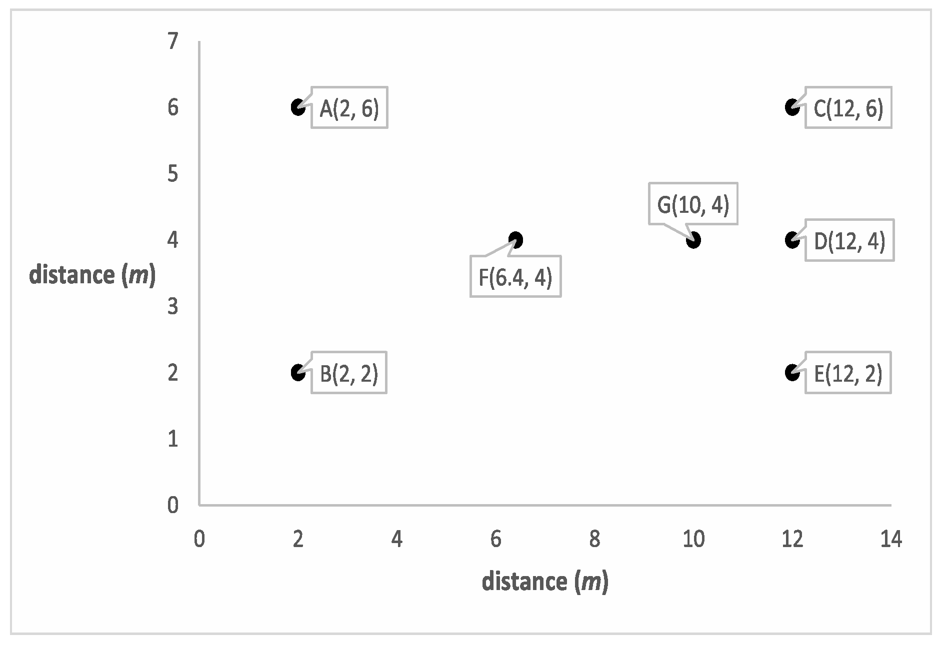
- Location suitability: This criterion measures how suitable a node location is as a CH with respect to surrounding nodes within a predefined range. A more suitable location for a CH node is a location with lower total communication energy.Location suitability for any node is measured by averaging the energy consumed locally by the sensor nodes located around the current node within a pre-defined range. We are interested in the nodes located within a predefined range as long as they are not closer in distance to any other pre-selected CH because they will be probably members of the current node if this current node wins CH election.Since we use the average of the consumed energies for the current node, we use the term average of local consumed energy and shorten it as to point out the location suitability. Note that we measure the average of the consumed energy rather than the total consumed energy to guarantee that the size of the group does not have an effect on the normalized value.Some consider, mistakenly, that if a node has a lower sum of distances to its future probable members, then is situated at a more suitable location to become CH. This stems from the assumption that the nodes closer to the centroid of the group will consume less total energy. However, since the energy is exponentially proportional to the distance, it becomes necessary to consider members with extreme distances. This means that the location with the minimum average distances to other surrounding nodes in a predefined range is not always the most suitable location for a node to become a CH since it may not always result in minimum total consumed energy for its surrounding group of nodes.To illustrate this idea, consider the scenario depicted in Figure 2. Here, node G has the minimum average distance of m from its surrounding nodes, and is the closest to the centroid. If selected as a CH, it will result in an average consumed energy of J, for one byte of data from each neighboring node. On the other hand, node F has an average distance of m, but results in an average consumed energy of J. For that reason, we base the computation of location suitability for a node to become a CH on the consumed energy rather than the total distances.
- Density of surrounding nodes: Selecting CHs surrounded by dense nodes over CHs surrounded by sparse nodes improves the energy consumption by increasing the opportunity for nodes with more neighbors in their vicinity to become CHs. Thereby, the local consumed energy for the group members is decreased.Density is calculated by the number of surrounding nodes within a predefined range normalized using Equation (1), where is the density of the current node, is the maximum density value through all candidate nodes, and is the minimum density value through all candidate nodes.
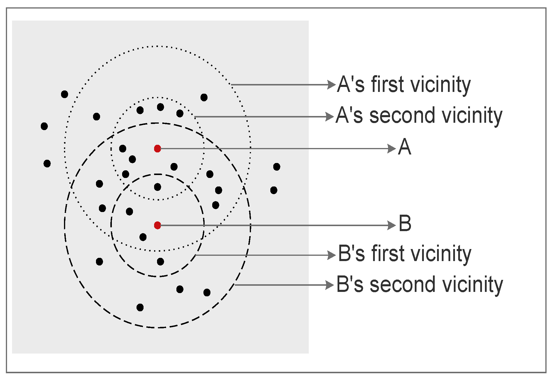
- Compaction of surrounding nodes: Group compaction is a measure of how the surrounding nodes are distributed around the current node. A node surrounded by more neighbors in a closer vicinity is considered of higher compactiondegree. Selecting a node with a higher compactiondegree minimizes the total energy consumption. This criterion is important to assign different priorities for CH candidates with the same number of surrounding nodes within a predefined range. In other words, it is beneficial for distinguishing candidates surrounded by the same density of sensor nodes.Compaction is calculated as the ratio of the number of nodes located within the first vicinity region to those located within the second vicinity region. The first vicinity region is that region that is within half of a predefined radius distance, whereas the second vicinity region is the one that is within the nodes’ radius.As shown in Figure 3, the small circles surrounding A and B are considered as the first vicinities, and the larger ones are considered as the second vicinities for nodes A and B. The distance to which to extend the first vicinity is a design parameter and may be any fraction of the radius.To normalize the Compaction, we use Equation (1), where is the Compaction value of current node, is the maximum Compaction value through all candidate nodes, and is the minimum compaction value through all candidate nodes.
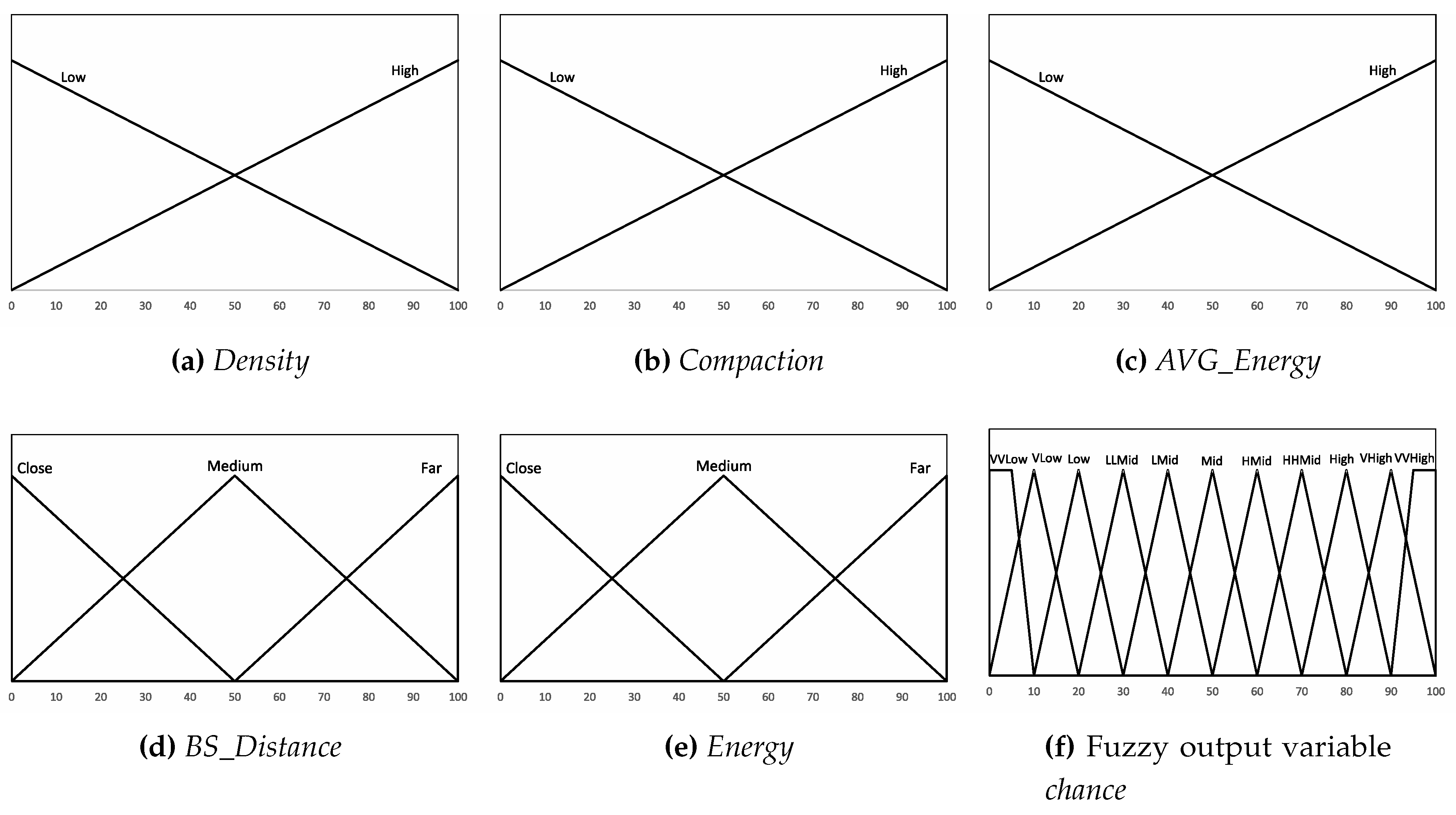
3.2. Fuzzy Sets
3.3. The Proposed Clustering Technique FL-EEC/D
| Algorithm 1 Calculation of the minimum forced distance between CHs. | |
| functionCalc_Min_Dist() | N: List of live nodes |
| p: percentage of CHs in WSN | |
| : length of X-dimension, : Length of Y-dimension | |
| ← | : desired # of clusters |
| c ← 1 | c: # of of regional columns, initially set to 1 |
| r ← 1 | r: # of regional rows, initially set to 1 |
| ← | : difference between # of created rectangles and the desired # of clusters, initially set to |
| I ← 1 | |
| while do | |
| J ← I | |
| while do | |
| if then | |
| ← | |
| c ← I | |
| r ← J | |
| end if | |
| J ← | |
| end while | |
| I ← | |
| end while | |
| ← | |
| ← | |
| d ← | |
| return d | d: minimum distance between CHs |
| end function | |
| Algorithm 2 Clustering based on minimum separation distance enforcement between CHs. | |
| procedureWSN clustering | |
| inputs: | |
| % N: set of live nodes % | |
| ← d | % d: minimum forced distance % |
| p | % p: Percentage of live nodes to become CHs % |
| ← | % : number of the desired CHs % |
| outputs: | |
| % set of CHs % | |
| % set of clusters % | |
| steps: | |
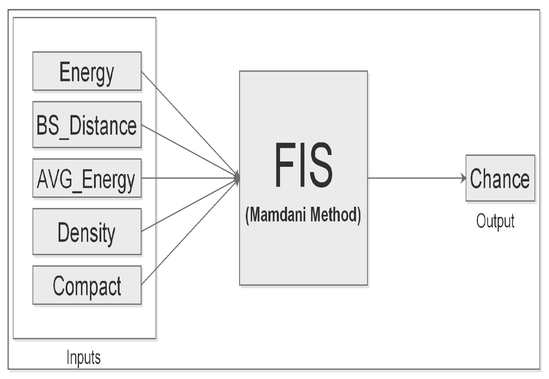
| 1) For each node , if the distance from to the closest already selected is less than d, then calculate each of the fuzzy input variables: Energy, BS_Distance, Density, Compaction AVG_Energy. | |
| 2) Calculate the fuzzy output variable chance for each based on the linguistic variables using the proposed fuzzy inference system | |
| 3) Select with the highest chance value among the nodes located away from any pre-selected by the distance d | |
| 4) Repeat Steps 1–4 until reaching | |
| 5) Form clusters, , by joining each to the closest | |
| end procedure | |
4. Performance Evaluation
4.1. Simulation Parameters
4.2. Network Model
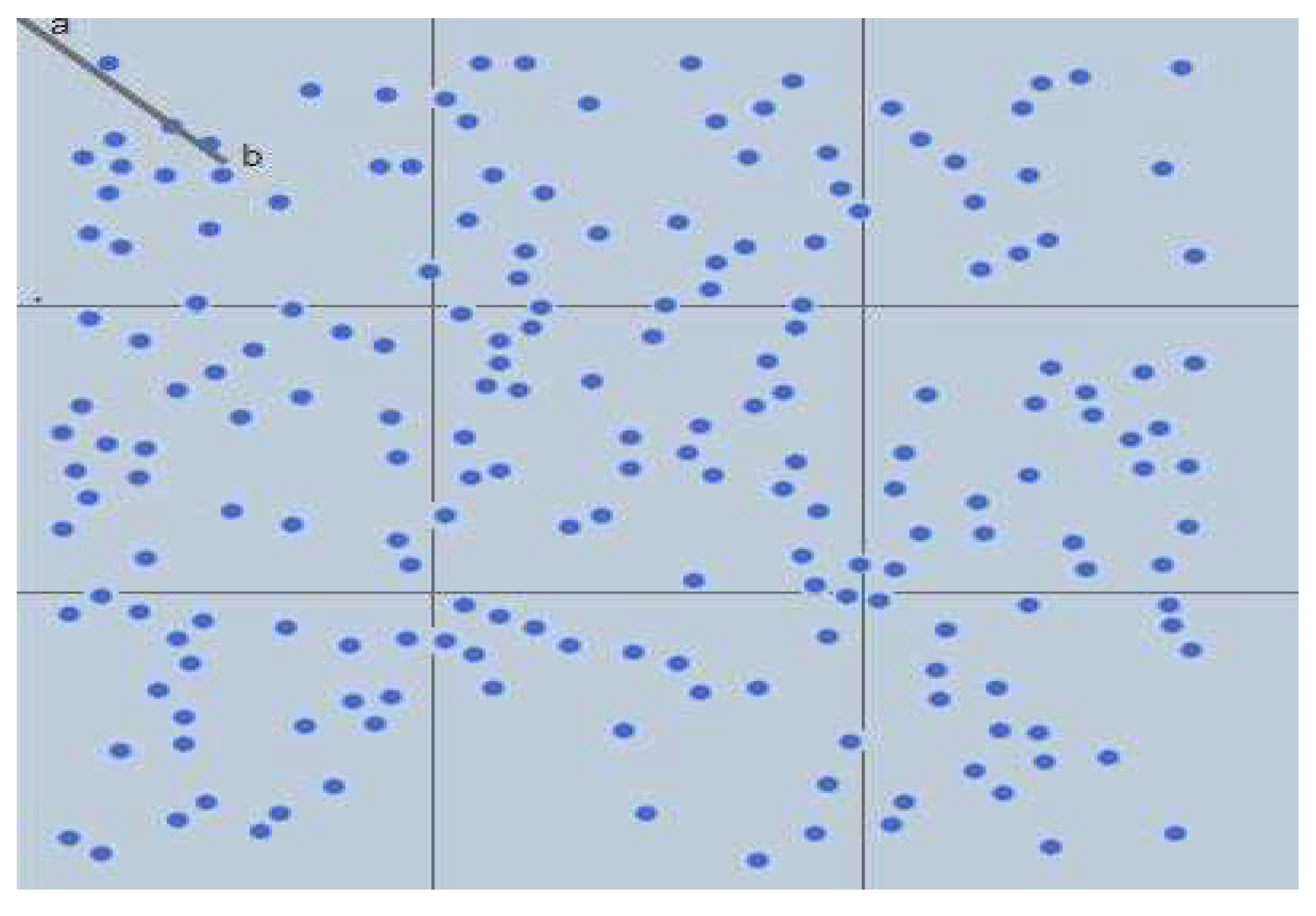
- All sensor nodes are randomly distributed over a two-dimensional area.
- All sensor nodes are homogeneous in terms of processing and communication capabilities. Furthermore, they have the same battery, radio, sensing, and storage capabilities.
- There are no recharging capabilities.
- The BS is able to estimate the locations of the sensor nodes by using any localization technique. This may be based on utilizing GPS [57,58] or by adopting GPS-free localization such as weighted centroid localization [59,60,61], which is based on the received signal strength. Generally, a small error in localization will not be significant for the overall clustering result since the values are calculated as relative variances between the lowest and highest values. These relative variances are later fuzzified (expressed as linguistic variables). The percentage of cluster heads is supposed to be 5% of the total number of sensor nodes in the WSN.
- Cluster heads are re-selected periodically.
4.3. Performance Metrics
4.4. Evaluation of FL-ECC/D
5. Conclusions and Future Work
Author Contributions
Funding
Conflicts of Interest
Abbreviations
| WSN | Wireless Sensor Network |
| CH | Cluster Head |
| BS | Base Station |
| FL-EEC/D | Fuzzy Logic-based Energy-Efficient Clustering based on minimum separation Distance enforcement between CHs |
| LEACH | Low Energy Adaptive Clustering Hierarchy |
| FIS | Fuzzy Inference System |
| HRP | Hierarchical Routing Protocols |
| PEGASIS | Power-Efficient Gathering in Sensor Information Systems |
| DPSO | Discrete Particle Swarm Optimization |
| FND | First Node Dead |
| 10PND | 10% of Nodes Dead |
| QND | Quarter of Nodes Dead |
| HND | Half of Nodes Dead |
References
- Buratti, C.; Conti, A.; Dardari, D.; Verdone, R. An overview on wireless sensor networks technology and evolution. Sensors 2009, 9, 6869–6896. [Google Scholar] [CrossRef] [PubMed]
- Giorgetti, A.; Lucchi, M.; Tavelli, E.; Barla, M.; Gigli, G.; Casagli, N.; Chiani, M.; Dardari, D. A robust wireless sensor network for landslide risk analysis: system design, deployment, and field testing. IEEE Sens. J. 2016, 16, 6374–6386. [Google Scholar] [CrossRef]
- Rashid, B.; Rehmani, M.H. Applications of wireless sensor networks for urban areas: A survey. J. Netw. Comput. Appl. 2016, 60, 192–219. [Google Scholar] [CrossRef]
- Modieginyane, K.M.; Letswamotse, B.B.; Malekian, R.; Abu-Mahfouz, A.M. Software defined wireless sensor networks application opportunities for efficient network management: A survey. Comput. Electr. Eng. 2018, 66, 274–287. [Google Scholar] [CrossRef]
- Puccinelli, D.; Haenggi, M. Wireless sensor networks: applications and challenges of ubiquitous sensing. IEEE Circuits Syst. Mag. 2005, 5, 19–31. [Google Scholar] [CrossRef]
- Younis, O.; Fahmy, S. HEED: A hybrid, energy-efficient, distributed clustering approach for ad hoc sensor networks. IEEE Trans. Mob. Comput. 2004, 3, 366–379. [Google Scholar] [CrossRef]
- Lindsey, S.; Raghavendra, C.S. PEGASIS: Power-efficient gathering in sensor information systems. In Proceedings of the IEEE Aerospace Conference Proceedings, Big Sky, MT, USA, 9–16 March 2002; Volume 3, p. 3. [Google Scholar]
- Hu, F.; Cao, X. Wireless Sensor Networks: Principles and Practice; CRC Press: Boca Raton, FL, USA, 2010. [Google Scholar]
- Heinzelman, W.B.; Chandrakasan, A.P.; Balakrishnan, H. An application-specific protocol architecture for wireless microsensor networks. IEEE Trans. Wirel. Commun. 2002, 1, 660–670. [Google Scholar] [CrossRef] [Green Version]
- Shurman, M.M.; Al-Mistarihi, M.F.; Harb, S. An Energy-Efficient Coverage Aware Clustering Mechanism for Wireless Sensor Networks. In Proceedings of the 5th International Conference on Communications, Computers and Applications (MIC-CCA 2012), Istanbul, Turkey, 12–14 October 2012. [Google Scholar]
- Shurman, M.M.; Al-Mistarihi, M.; Drabkh, K.; Naji, A. Hierarchal Clustering Using Genetic Algorithm in Wireless Sensor Networks. In Proceedings of the 36th International Convention on Information and Communication Technology, Electronics and Microelectronics (MIPRO2013), Opatija, Croatia, 20–24 May 2013. [Google Scholar]
- Heinzelman, W.R.; Chandrakasan, A.; Balakrishnan, H. Energy-efficient communication protocol for wireless microsensor networks. In Proceedings of the 33rd Annual Hawaii International Conference on System Sciences, Maui, HI, USA, 7 January 2000; p. 8020. [Google Scholar]
- Suhonen, J.; Kohvakka, M.; Kaseva, V.; Hämäläinen, T.D.; Hännikäinen, M. Low-Power Wireless Sensor Networks: Protocols, Services and Applications; Springer Science & Business Media: Berlin, Germany, 2012. [Google Scholar]
- Manap, Z.; Ali, B.M.; Ng, C.K.; Noordin, N.K.; Sali, A. A review on hierarchical routing protocols for wireless sensor networks. Wirel. Pers. Commun. 2013, 72, 1077–1104. [Google Scholar] [CrossRef]
- Pal, R.; Sharma, A.K. FSEP-E: Enhanced stable election protocol based on fuzzy Logic for cluster head selection in WSNs. In Proceedings of the 2013 Sixth International Conference on Contemporary Computing (IC3), Noida, India, 8–10 August 2013; pp. 427–432. [Google Scholar]
- Shurman, M.M.; Alomari, Z.; Mhaidat, K. An Efficient Billing Scheme for Trusted Nodes Using Fuzzy Logic in Wireless Sensor Networks. J. Wirel. Eng. Technol. 2014, 5, 62–73. [Google Scholar] [CrossRef]
- Barrett, G.F.; Crossley, T.F.; Worswick, C. Consumption and income inequality in Australia. Econ. Rec. 2000, 76, 116–138. [Google Scholar] [CrossRef]
- Akyildiz, I.F.; Su, W.; Sankarasubramaniam, Y.; Cayirci, E. Wireless sensor networks: A survey. Comput. Netw. 2002, 38, 393–422. [Google Scholar] [CrossRef]
- Shi, S.; Liu, X.; Gu, X. An energy-efficiency Optimized LEACH-C for wireless sensor networks. In Proceedings of the 7th International ICST Conference on Communications and Networking in China (CHINACOM), Kunming, China, 8–10 August 2012; pp. 487–492. [Google Scholar]
- Geetha, V.; Kallapur, P.V.; Tellajeera, S. Clustering in wireless sensor networks: Performance comparison of leach & leach-c protocols using ns2. Procedia Technol. 2012, 4, 163–170. [Google Scholar]
- Manjeshwar, A.; Agrawal, D.P. TEEN: A routing protocol for enhanced efficiency in wireless sensor networks. In Proceedings of the 15th International Parallel and Distributed Processing Symposium, San Francisco, CA, USA, 23–27 April 2001; pp. 2009–2015. [Google Scholar]
- Manjeshwar, A.; Agrawal, D.P. APTEEN: A hybrid protocol for efficient routing and comprehensive information retrieval in wireless sensor networks. In Proceedings of the International Parallel and Distributed Processing Symposium (IPDPS 2002), Fort Lauderdale, FL, USA, 15–19 April 2002; pp. 2009–2015. [Google Scholar]
- Liu, X. A survey on clustering routing protocols in wireless sensor networks. Sensors 2012, 12, 11113–11153. [Google Scholar] [CrossRef] [PubMed]
- Cheng, D.; Song, Y.; Mao, Y.; Wang, X. An energy efficient cluster-based routing protocol for intelligent environmental monitoring system. In Proceedings of the 2014 2nd International Conference on Systems and Informatics (ICSAI), Shanghai, China, 15–17 November 2014; pp. 505–509. [Google Scholar]
- Park, G.Y.; Kim, H.; Jeong, H.W.; Youn, H.Y. A novel cluster head selection method based on K-means algorithm for energy efficient wireless sensor network. In Proceedings of the 27th International Conference onAdvanced Information Networking and Applications Workshops (WAINA), Barcelona, Spain, 25–28 March 2013; pp. 910–915. [Google Scholar]
- Eshaftri, M.; Al-Dubai, A.Y.; Romdhani, I.; Yassien, M.B. A new energy efficient cluster based protocol for wireless sensor networks. In Proceedings of the 2015 Federated Conference on Computer Science and Information Systems (FedCSIS), Lodz, Poland, 13–16 September 2015; pp. 1209–1214. [Google Scholar]
- Li, L.Y.; Liu, C.D. An Improved Algorithm of LEACH Routing Protocol in Wireless Sensor Networks. In Proceedings of the 2014 8th International Conference on Future Generation Communication and Networking (FGCN), Haikou, China, 20–23 December 2014; pp. 45–48. [Google Scholar]
- Min, D.; Chun, X. An improved cluster protocol design method for low energy uneven wireless sensor network. In Proceedings of the 2015 International Conference on Computer and Computational Sciences (ICCCS), Noida, India, 27–29 January 2015; pp. 189–192. [Google Scholar]
- Li, J.; Liu, D. DPSO-based clustering routing algorithm for energy harvesting wireless sensor networks. In Proceedings of the 2015 International Conference on Wireless Communications & Signal Processing (WCSP), Nanjing, China, 15–17 October 2015; pp. 1–5. [Google Scholar]
- Prabhavathi, S.; Subramanyam, A.; Rao, A.A. Clustering process for maximizing lifetime using probabilistic logic in WSN. In Proceedings of the 2014 International Conference on Computing, Communication and Networking Technologies (ICCCNT), Hefei, China, 11–13 July 2014; pp. 1–7. [Google Scholar]
- Elhabyan, R.S.; Yagoub, M.C. Evolutionary algorithms for cluster heads election in wireless sensor networks: Performance comparison. In Proceedings of the Science and Information Conference (SAI), London, UK, 28–30 July 2015; pp. 1070–1076. [Google Scholar]
- Randriatsiferana, R.S.; Alicalapa, F.; Lorion, R.; Mohammed, A.M. A clustering algorithm based on energy variance and coverage density in centralized hierarchical Wireless Sensor Networks. In Proceedings of the AFRICON, Pointe-Aux-Piments, Mauritius, 9–12 September 2013; pp. 1–5. [Google Scholar]
- Singh, D.P.; Bhateja, V.; Soni, S.K. Prolonging the lifetime of wireless sensor networks using prediction based data reduction scheme. In Proceedings of the 2014 International Conference on Signal Processing and Integrated Networks (SPIN), Noida, India, 20–21 February 2014; pp. 420–425. [Google Scholar]
- Belghith, O.B.; Sbita, L. Extending the network lifetime of wireless sensor networks using fuzzy logic. In Proceedings of the 12th International Multi-Conference on Systems, Signals & Devices (SSD), Mahdia, Tunisia, 16–19 March 2015; pp. 1–5. [Google Scholar]
- Nayak, P.; Devulapalli, A. A fuzzy logic-based clustering algorithm for wsn to extend the network lifetime. IEEE Sens. J. 2016, 16, 137–144. [Google Scholar] [CrossRef]
- Bagci, H.; Yazici, A. An energy aware fuzzy unequal clustering algorithm for wireless sensor networks. In Proceedings of the 2010 IEEE International Conference on Fuzzy Systems (FUZZ), Barcelona, Spain, 18–23 July 2010; pp. 1–8. [Google Scholar]
- Siew, Z.; Liau, C.F.; Kiring, A.; Arifianto, M.; Teo, K.T.K. Fuzzy logic based cluster head election for wireless sensor network. In Proceedings of the 3rd CUTSE International Conference, Sarawak, Malaysia, 8–9 November 2011; pp. 301–306. [Google Scholar]
- Pires, A.; Silva, C.; Cerqueira, E.; Monteiro, D.; Viegas, R. CHEATS: A cluster-head election algorithm for WSN using a Takagi-Sugeno fuzzy system. In Proceedings of the 2011 IEEE Latin-American Conference on Communications (LATINCOM), Belem, Brazil, 26–28 October 2011; pp. 1–6. [Google Scholar]
- Fu, Z. Cluster head election with a fuzzy algorithm for wireless sensor networks. In Proceedings of the 2013 6th International Congress on Image and Signal Processing (CISP), Hangzhou, China, 16–18 December 2013; Volume 3, pp. 1427–1431. [Google Scholar]
- Gupta, I.; Riordan, D.; Sampalli, S. Cluster-head election using fuzzy logic for wireless sensor networks. In Proceedings of the 3rd Annual Communication Networks and Services Research Conference, Halifax, NS, Canada, 16–18 May 2005; pp. 255–260. [Google Scholar]
- Chourasia, M.K.; Panchal, M.; Shrivastav, A. Energy efficient protocol for mobile Wireless Sensor Networks. In Proceedings of the Communication, Control and Intelligent Systems (CCIS), Mathura, India, 7–8 November 2015; pp. 79–84. [Google Scholar]
- Preethiya, T.; Santhi, G. Enhancement of lifetime using fuzzy-Based clustering approach in WSN. In Proceedings of the 2014 International Conference on Electronics and Communication Systems (ICECS), Coimbatore, India, 13–14 February 2014; pp. 1–5. [Google Scholar]
- Islam, M.K. Energy Aware Techniques for Certain Problems in Wireless Sensor Networks. Ph.D. Thesis, School of Computing, Queens University, Shenzhen, China, 2010. [Google Scholar]
- Alla, S.B.; Ezzati, A.; Mohsen, A. Gateway and cluster head election using fuzzy logic in heterogeneous wireless sensor networks. In Proceedings of the 2012 International Conference on Multimedia Computing and Systems (ICMCS), Tangier, Morocco, 10–12 May 2012; pp. 761–766. [Google Scholar]
- Khan, F.U.; Shah, I.A.; Jan, S.; Khan, I.; Mehmood, M.A. Fuzzy logic based cluster head selection for homogeneous wireless sensor networks. In Proceedings of the 2015 International Conference on Open Source Systems & Technologies (ICOSST), Lahore, Pakistan, 17–19 December 2015; pp. 41–45. [Google Scholar]
- Messaoudi, A.; Elkamel, R.; Helali, A.; Bouallegue, R. Distributed fuzzy logic based routing protocol for wireless sensor networks. In Proceedings of the 24th International Conference on Software, Telecommunications and Computer Networks (SoftCOM), Split, Croatia, 22–24 September 2016; pp. 1–7. [Google Scholar]
- Singh, S.; Panchal, M.; Jain, R. Fuzzy Logic Based Energy Efficient Network Lifetime Optimization in Wireless Sensor Network. In Proceedings of the 2016 International Conference on Micro-Electronics and Telecommunication Engineering (ICMETE), Ghaziabad, India, 22–23 September 2016; pp. 493–498. [Google Scholar]
- Buratti, C.; Giorgetti, A.; Verdone, R. Cross-layer design of an energy-efficient cluster formation algorithm with carrier-sensing multiple access for wireless sensor networks. EURASIP J. Wirel. Commun. Netw. 2005, 2005, 672–685. [Google Scholar] [CrossRef]
- Li, N.; Martínez, J.F.; Díaz, V.H. The balanced cross-layer design routing algorithm in wireless sensor networks using fuzzy logic. Sensors 2015, 15, 19541–19559. [Google Scholar] [CrossRef]
- Zuo, J.; Dong, C.; Ng, S.X.; Yang, L.L.; Hanzo, L. Cross-layer aided energy-efficient routing design for ad hoc networks. IEEE Commun. Surv. Tutor. 2015, 17, 1214–1238. [Google Scholar] [CrossRef]
- Li, N.; Martínez-Ortega, J.F.; Díaz, V.H. Cross-Layer and Reliable Opportunistic Routing Algorithm for Mobile Ad Hoc Networks. IEEE Sens. J. 2018, 18, 5595. [Google Scholar] [CrossRef]
- Zhang, Y.; Wang, J.; Han, D.; Wu, H.; Zhou, R. Fuzzy-logic based distributed energy-efficient clustering algorithm for wireless sensor networks. Sensors 2017, 17, 1554. [Google Scholar] [CrossRef]
- Mohamad, I.B.; Usman, D. Standardization and its effects on K-means clustering algorithm. Res. J. Appl. Sci. Eng. Technol. 2013, 6, 3299–3303. [Google Scholar] [CrossRef]
- Grus, J. Data Science from Scratch: First Principles with Python; O’Reilly Media, Inc.: Sebastopol, CA, USA, 2015. [Google Scholar]
- Ioffe, S.; Szegedy, C. Batch normalization: Accelerating deep network training by reducing internal covariate shift. arXiv, 2015; arXiv:1502.03167. [Google Scholar]
- Banimelhem, O.; Taqieddin, E.; Mowafi, M.Y.; Awad, F. Fuzzy Logic-Based Cluster Heads Percentage Calculation for Improving the Performance of the LEACH Protocol. In Fuzzy Systems: Concepts, Methodologies, Tools, and Applications; IGI Global: Hershey, PA, USA, 2017; pp. 609–627. [Google Scholar]
- Cheng, B.; Du, R.; Yang, B.; Yu, W.; Chen, C.; Guan, X. An accurate GPS-based localization in wireless sensor networks: A GM-WLS method. In Proceedings of the 2011 International Conference on Parallel Processing Workshops, Taipei, Taiwan, 13–16 September 2011; pp. 33–41. [Google Scholar]
- Stoleru, R.; He, T.; Stankovic, J.A. Walking GPS: A practical solution for localization in manually deployed wireless sensor networks. In Proceedings of the 29th Annual IEEE International Conference on Local Computer Networks, Tampa, FL, USA, 16–18 November 2004; pp. 480–489. [Google Scholar]
- Magowe, K.; Giorgetti, A.; Kandeepan, S.; Yu, X. Accurate analysis of weighted centroid localization. IEEE Trans. Cognit. Commun. Netw. 2018. [Google Scholar] [CrossRef]
- Wang, L.; Xu, Q. GPS-free localization algorithm for wireless sensor networks. Sensors 2010, 10, 5899–5926. [Google Scholar] [CrossRef] [PubMed]
- Giorgetti, A.; Magowe, K.; Kandeepan, S. Exact analysis of weighted centroid localization. In Proceedings of the 2016 24th European Signal Processing Conference (EUSIPCO), Budapest, Hungary, 28 August–2 September 2016; pp. 743–747. [Google Scholar]
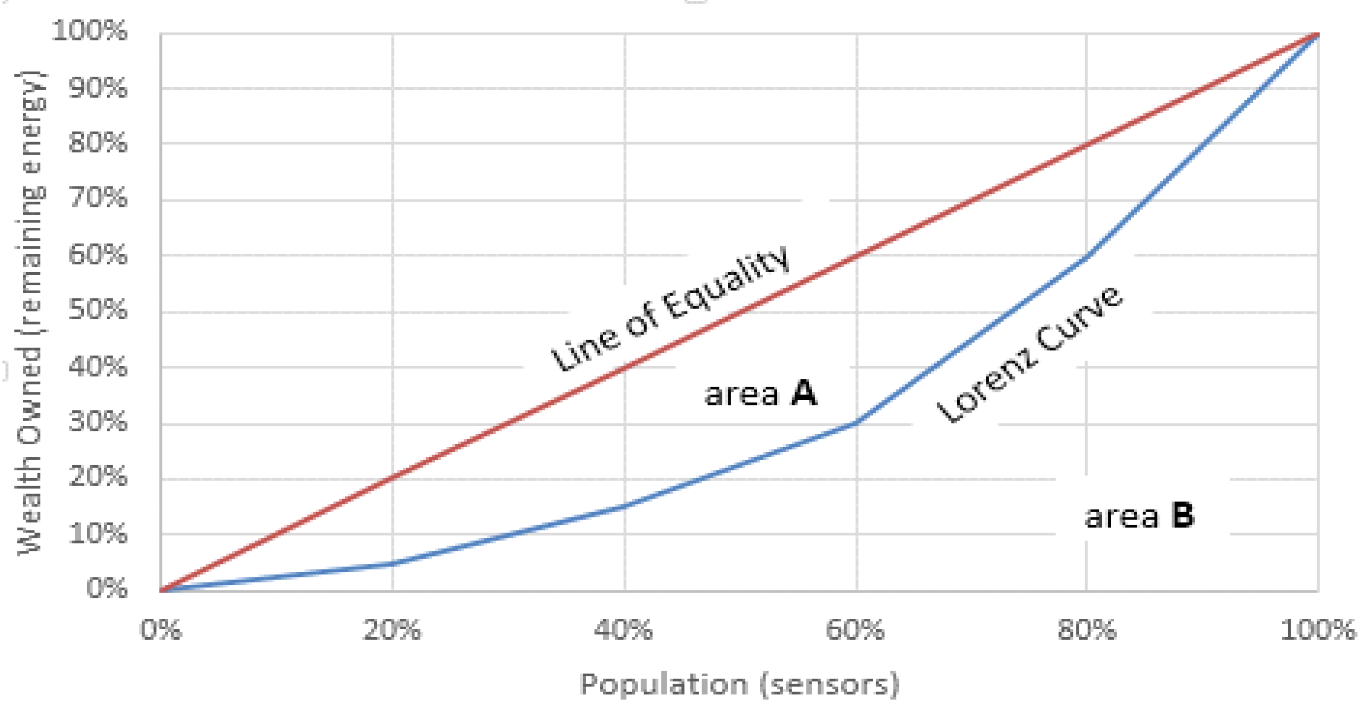
- Gastwirth, J. A General Definition of the Lorenz Curve. Econometrica 1971, 39, 1037–1039. [Google Scholar] [CrossRef]


| Class | Single Layer | Cross Layer | |
|---|---|---|---|
| Cluster Based | Centralized | Sensors are organized into clusters, and transmissions go through CHs. In this approach, node locations are estimated by the BS. This benefits from the global knowledge of the network and achieves a more efficient clustering compared to the distributed approach. Examples appear in [19,25,26,29], and [32]. | Information is collected and combined from different network layers to be utilized for CH election. The works in [49] and [51] follow this approach. |
| Distributed | Sensors are organized into clusters in a distributed manner, and transmissions go through CHs. A drawback of this approach is that it is confined to local information, and this may lead to non-optimal WSN clustering [6,12,24,27,52]. | ||
| Chain Based | Proactive | Sensors are periodically organized into chains through which the transmissions pass. An example of this approach is found in [7]. | |
| Reactive | Sensors are organized as chains through which the transmissions pass. Routes change immediately in response to the changes of relevant parameters of interest [21]. | ||
| SN. | Input Variables | Output Variable | ||||
|---|---|---|---|---|---|---|
| Energy | BS_Distance | AVG_Energy | Density | Compaction | Chance | |
| 1 | Low | Close | Low | Low | Low | LMid |
| 2 | Low | Close | Low | Low | High | HMid |
| 3 | Low | Close | Low | High | Low | HMid |
| 4 | Low | Close | Low | High | High | High |
| 5 | Low | Close | High | Low | Low | Low |
| 6 | Low | Close | High | Low | High | LMid |
| 7 | Low | Close | High | High | Low | LMid |
| 8 | Low | Close | High | High | High | HMid |
| 9 | Low | Medium | Low | Low | Low | VVLow |
| 10 | Low | Medium | Low | Low | High | VLow |
| 11 | Low | Medium | Low | High | Low | VLow |
| 12 | Low | Medium | Low | High | High | LLMid |
| 13 | Low | Medium | High | Low | Low | VVLow |
| 14 | Low | Medium | High | Low | High | VVLow |
| 15 | Low | Medium | High | High | Low | VVLow |
| 16 | Low | Medium | High | High | High | VLow |
| 17 | Low | Far | Low | Low | Low | VVLow |
| 18 | Low | Far | Low | Low | High | VVLow |
| 19 | Low | Far | Low | High | Low | VVLow |
| 20 | Low | Far | Low | High | High | VVLow |
| 21 | Low | Far | High | Low | Low | VVLow |
| 22 | Low | Far | High | Low | High | VVLow |
| 23 | Low | Far | High | High | Low | VVLow |
| 24 | Low | Far | High | High | High | VVLow |
| 25 | Medium | Close | Low | Low | Low | High |
| 26 | Medium | Close | Low | Low | High | VVHigh |
| 27 | Medium | Close | Low | High | Low | VVHigh |
| 28 | Medium | Close | Low | High | High | VVHigh |
| 29 | Medium | Close | High | Low | Low | HMid |
| 30 | Medium | Close | High | Low | High | High |
| 31 | Medium | Close | High | High | Low | High |
| 32 | Medium | Close | High | High | High | VVHigh |
| 33 | Medium | Medium | Low | Low | Low | LLMid |
| 34 | Medium | Medium | Low | Low | High | Mid |
| 35 | Medium | Medium | Low | High | Low | Mid |
| 36 | Medium | Medium | Low | High | High | HHMid |
| 37 | Medium | Medium | High | Low | Low | VLow |
| 38 | Medium | Medium | High | Low | High | LLMid |
| 39 | Medium | Medium | High | High | Low | LLMid |
| 40 | Medium | Medium | High | High | High | Mid |
| 41 | Medium | Far | Low | Low | Low | VVLow |
| 42 | Medium | Far | Low | Low | High | VVLow |
| 43 | Medium | Far | Low | High | Low | VVLow |
| 44 | Medium | Far | Low | High | High | Low |
| 45 | Medium | Far | High | Low | Low | VVLow |
| 46 | Medium | Far | High | Low | High | VVLow |
| 47 | Medium | Far | High | High | Low | VVLow |
| 48 | Medium | Far | High | High | High | VVLow |
| 49 | High | Close | Low | Low | Low | VVHigh |
| 50 | High | Close | Low | Low | High | VVHigh |
| 51 | High | Close | Low | High | Low | VVHigh |
| 52 | High | Close | Low | High | High | VVHigh |
| 53 | High | Close | High | Low | Low | VVHigh |
| 54 | High | Close | High | Low | High | VVHigh |
| 55 | High | Close | High | High | Low | VVHigh |
| 56 | High | Close | High | High | High | VVHigh |
| 57 | High | Medium | Low | Low | Low | HHMid |
| 58 | High | Medium | Low | Low | High | VHigh |
| 59 | High | Medium | Low | High | Low | VHigh |
| 60 | High | Medium | Low | High | High | VVHigh |
| 61 | High | Medium | High | Low | Low | Mid |
| 62 | High | Medium | High | Low | High | HHMid |
| 63 | High | Medium | High | High | Low | HHMid |
| 64 | High | Medium | High | High | High | VHigh |
| 65 | High | Far | Low | Low | Low | Low |
| 66 | High | Far | Low | Low | High | LMid |
| 67 | High | Far | Low | High | Low | LMid |
| 68 | High | Far | Low | High | High | HMid |
| 69 | High | Far | High | Low | Low | VVLow |
| 70 | High | Far | High | Low | High | Low |
| 71 | High | Far | High | High | Low | Low |
| 72 | High | Far | High | High | High | LMid |
| Parameter | Value |
|---|---|
| Data Packet Size | 500 bytes |
| Initial Energy | 2 J |
| 50 nJ/bit | |
| 10 nJ/bit/m bytes | |
| 5 nJ/bit/signal | |
| 0.0013 nJ/bit/m | |
| Threshold Distance | 87 m |
| Deployment Method | Random |
© 2019 by the authors. Licensee MDPI, Basel, Switzerland. This article is an open access article distributed under the terms and conditions of the Creative Commons Attribution (CC BY) license (http://creativecommons.org/licenses/by/4.0/).
Share and Cite
Hamzah, A.; Shurman, M.; Al-Jarrah, O.; Taqieddin, E. Energy-Efficient Fuzzy-Logic-Based Clustering Technique for Hierarchical Routing Protocols in Wireless Sensor Networks. Sensors 2019, 19, 561. https://doi.org/10.3390/s19030561
Hamzah A, Shurman M, Al-Jarrah O, Taqieddin E. Energy-Efficient Fuzzy-Logic-Based Clustering Technique for Hierarchical Routing Protocols in Wireless Sensor Networks. Sensors. 2019; 19(3):561. https://doi.org/10.3390/s19030561
Chicago/Turabian StyleHamzah, Abdulmughni, Mohammad Shurman, Omar Al-Jarrah, and Eyad Taqieddin. 2019. "Energy-Efficient Fuzzy-Logic-Based Clustering Technique for Hierarchical Routing Protocols in Wireless Sensor Networks" Sensors 19, no. 3: 561. https://doi.org/10.3390/s19030561
APA StyleHamzah, A., Shurman, M., Al-Jarrah, O., & Taqieddin, E. (2019). Energy-Efficient Fuzzy-Logic-Based Clustering Technique for Hierarchical Routing Protocols in Wireless Sensor Networks. Sensors, 19(3), 561. https://doi.org/10.3390/s19030561