Mathematical Models of Critical Soft Error in Synchronous and Self-Timed Pipeline

Abstract

This paper analyzes the impact of a single soft error on the performance of a synchronous and self-timed pipeline. A nuclear particle running through the integrated circuit body is considered the most probable soft error source. The existing estimates show that self-timed circuits offer an advantage in terms of single soft error tolerance. The paper proves these estimates on the basis of a comparative probability analysis of a critical fault in two types of pipelines. The mathematical models derived in the paper describe the probability of a critical fault depending on the circuit’s characteristics, its operating discipline, and the soft error parameters. The self-timed pipeline operates in accordance with a two-phase discipline, based on the request–acknowledge interaction within the pipeline’s stages, which provides it with increased immunity to soft errors. Quantitative calculations performed on the basis of the derived mathematical models show that the self-timed pipeline has about 6.1 times better tolerance to a single soft error in comparison to its synchronous counterpart. The obtained results are in good agreement with empirical estimates of the soft error tolerance level of synchronous and self-timed circuits.

1. Introduction

The reliability of electronic equipment, including soft errors (SEs), is one of the most important characteristics of hardware, especially in adverse operating conditions. Cosmic rays, radiation, and nuclear particles are the causes of SEs in digital circuits in computing and control systems in most cases [1,2,3]. A soft error is expressed in the inversion of a signal logical level. It becomes critical if it leads to distortion of the initial data processing result or a pipeline stall.

Among all possible faults associated with external influences, SEs constitute the predominant part. Research has shown [1] that in integrated circuits, SEs are the cause of spacecraft on-board system failures in 95% of cases. With scaling down the design rules, the probability of SE occurrence increases [4], and SEs occur several orders of magnitude more often than failures [5]. A similar ratio of SEs and failures is observed in information systems [6]. Therefore, the development of methods for increasing the fault tolerance of digital circuit components and units is relevant and a priority. Soft error tolerance in this case is understood as the circuit’s ability to continue correct operation when an SE occurs, without loss or corruption of the processed data.

Over the past few decades, the response of digital circuits to SEs has been actively studied [7,8,9], and methods for protecting against SEs have been developed [10,11,12]. To increase the circuit’s immunity to SEs, correction codes [13,14], self-correcting circuits [15] providing automatic correction of SE-induced errors, electrical and time masking [16], and special circuit solutions for typical digital cells and units [17,18,19,20,21] are used. Methods to protect against SEs based on the circuit’s hardware redundancy, such as duplication [22], tripling [23], and “M-of-N” voting [24], are very popular.

Hardware redundancy increases the level of digital circuit immunity to SEs by means of SE control and masking tools built into the circuit. Asynchronous circuits operating on the principles of request–acknowledge interactions are initially hardware redundant. This ensures the circuit’s correct operation control [25,26,27]. Self-timed (ST) circuits, which belong to the subclass of quasi-delay-insensitive asynchronous circuits, have the maximum immunity to SEs with acceptable hardware costs [28,29]. Due to hardware redundancy, they demonstrate a higher fault tolerance level compared to synchronous and asynchronous counterparts [30].

Publications in recent years [30,31,32] have consider the digital circuit’s SE tolerance “in the first approximation” based on speculative estimates of the digital circuit’s response to an SE. References [33,34] use SE emulation to estimate fault tolerance, which allows critical circuit parts to be identified and the probability of SE propagation to the circuit’s outputs to be determined using multiple modeling sessions. There are probabilistic methods that estimate the SE’s observability [35,36] at the level of individual logical cells, large blocks, and systems [37,38]. They are similar to functional analysis and logical function system simulation.

This paper’s objective is to construct a mathematical model for calculating the probability of a single SE turning into a critical fault in a digital synchronous and ST circuit at a constant nuclear particle flux density as the most dangerous source of SEs [39]. Qualitative estimates show that ST circuits have a much higher immunity level to SEs compared to their synchronous counterparts [30,40]. However, they are empiric and based on approximately accounting for the event probabilities accompanying the SE’s occurrence and its propagation throughout the circuit. In particular, to calculate the probability, a speculative analysis of the outcome binary “tree” of the specified events is used, in which each outcome has a probability of 0.5. This article solves the current problem of theoretically assessing the probability of a critical SE occurrence by constructing a mathematical model for synchronous and ST pipelines. The proposed model can be used to determine and compare the digital synchronous and ST circuits’ SE tolerance levels.

The scientific novelty of the paper is as follows:

• Mathematical models of the critical SE occurrence caused by a nuclear particle run through the body of the circuit chip in the synchronous and ST pipeline stages were obtained.
• A comparative analysis of the synchronous and ST pipelines’ SE tolerance was carried out based on analytical estimates, taking into account hardware costs for the typical parameter values of the circuit components and SE characteristics.

2. Statement of the Problem

Modern high-performance computing and control systems have a pipeline structure. Therefore, we chose synchronous and ST pipelines as the objects for constructing a critical SE mathematical model. Figure 1 shows a typical synchronous pipeline block diagram. Here, D_in is the input data; D_out is the output data; and Clk is the global clock signal. Figure 2 shows a typical ST pipeline block diagram. Here, Ack_i is the signal acknowledging the completion of the phase transition in the first pipeline stage and Ack_o is the signal acknowledging the completion of the phase transition in the output data D_out receiver.

The stages of both pipeline types consist of a combinational part (CP) and an output register (Rg). In the ST pipeline, the CP and register include an indication part (Ind), which generates signals acknowledging the CP and register switching completion to the current phase. The Muller’s C-element [26] combines these signals into stage indication output. In the synchronous pipeline, the register bit is implemented on a D flip-flop, while in the ST pipeline it is implemented on two modified two-input C-elements [41].

The ST pipeline stage operates according to a two-phase discipline, including working and spacer phases [28]. It uses an indication subcircuit to detect the completion of all transitions, initiated during the stage switching to the current operation phase. The entire operating cycle of the ST pipeline stage can be divided into four consecutive intervals:

• Stage data output transition to a working phase (I₁);
• Stage’s indication output working value generation (I₂);
• Stage data output transition to a spacer phase (I₃);
• Stage’s indication output spacer value generation (I₄).

SEs can appear both in the CP stage and the register at any ST stage in the operation cycle interval. It becomes critical if it leads to pipeline output result corruption or “hanging” of the data processing, which is possible in the ST pipeline. The paper’s purpose is to create a stochastic mathematical model of the occurrence of critical SEs in the synchronous and ST pipeline stages because of the impact of nuclear particles.

3. Initial Hypotheses

The development of critical fault mathematical models rests on the following initial hypotheses:

• The density ${\gamma }_{NP}$ of the nuclear particle flux that is the SE source is constant in time and within the pipeline layout area. The characteristics of the nuclear particle flux, including its density, depend on the circuit’s operating conditions. The adopted assumption corresponds to the most practical applications.
• Each nuclear particle causes the appearance of an SE, which is not necessarily critical, with probability $P_{NP}$, and at any moment in time no more than one SE is observed in the circuit. Such hypotheses average the conditions of an SE caused by an interaction with the semiconductor, determined by the particle’s incidence angle on the semiconductor’s surface, its energy, the type of active semiconductor structure affected by the particle, and so on.
• An SE’s duration is described by the Gaussian law with the probability density function:

  $$f(T_{SE})={\displaystyle \frac{e^{-\frac{{\left(T_{SE}-m_{SE}\right)}^2}{2{\sigma }_{SE}^2}}}{{\sigma }_{SE}\sqrt{2\pi }}},$$

  (1)

  where $T_{SE}$ is the SE duration; $m_{SE}$ is the mathematical expectation of $T_{SE}$; and ${\sigma }_{SE}$ is the standard deviation of $T_{SE}$.
• The average probability that stage CP does not mask an SE logically equals $P_{NM}$. In a specific circuit, this probability is determined by the circuit hardware complexity and the input data set processed by the circuit when a particle hits it. However, the accepted hypothesis allows one to draw a generalized conclusion in relation to a comparison of the synchronous and ST circuits’ reactions to the SE’s impact.

An SE’s duration is mainly determined by the particle energy. This fact has predetermined the choice of Gauss’ law to describe it. For example, in nuclear physics, Gauss’s law describes the distribution of the mean track length of heavy charged particles in matter and the signal pulse amplitude recording the particle track, which are also determined by the particle energy [42]. The SE’s duration is a positive value, so Gauss’s law describes it with some error. Since the area of the figure bounded by the probability density function curve and the abscissa axis on the interval (0, ∞) is less than 1, this error is taken into account when calculating the SE probability using Equation (1) by means of a normalizing coefficient $K_{err}$:

$$K_{err}=1-{\displaystyle \frac{1}{{\sigma }_{SE}\sqrt{2\pi }}}{\displaystyle \underset{-\infty }{\overset{0}{\int }}{e}^{-\frac{{\left(x-m_{SE}\right)}^2}{2{\sigma }_{SE}^2}}dx}.$$

(2)

If $m_{SE}>3{\sigma }_{SE}$, then the error can be neglected ($K_{err}$ = 1).

Based on the adopted initial hypotheses, let us estimate the probabilities of a critical SE occurring in the synchronous and ST pipeline stages depending on the SE’s characteristics (duration, time, and place of occurrence) and the cell delay parameters of the analyzed stages.

4. Critical Soft Errors in the Synchronous Pipeline Stage

Let us introduce the set of variables that we operate with to estimate the SE probability in synchronous circuits, which is presented in

Table 1. Variables for calculating SE probability in synchronous circuits.

Variable	Name
Clock period	$T_C$
An SE’s appearance time relative to the last active clock edge	$t_S$
Signal propagation delay from the faulty element to the stage register inputs	$t_{DS}$
Critical path delay of the stage’s CP in the worst case	$T_{\max }$
Performance reserve factor	$k_P$
Inverter switching delay	$t_I$
Die area of the stage’s CP	$S_{CP\_S}$
Die area of the stage’s register	$S_{R\_S}$

. The performance reserve factor equals $k_P={\displaystyle \frac{T_{\max }}{T_C}}$.

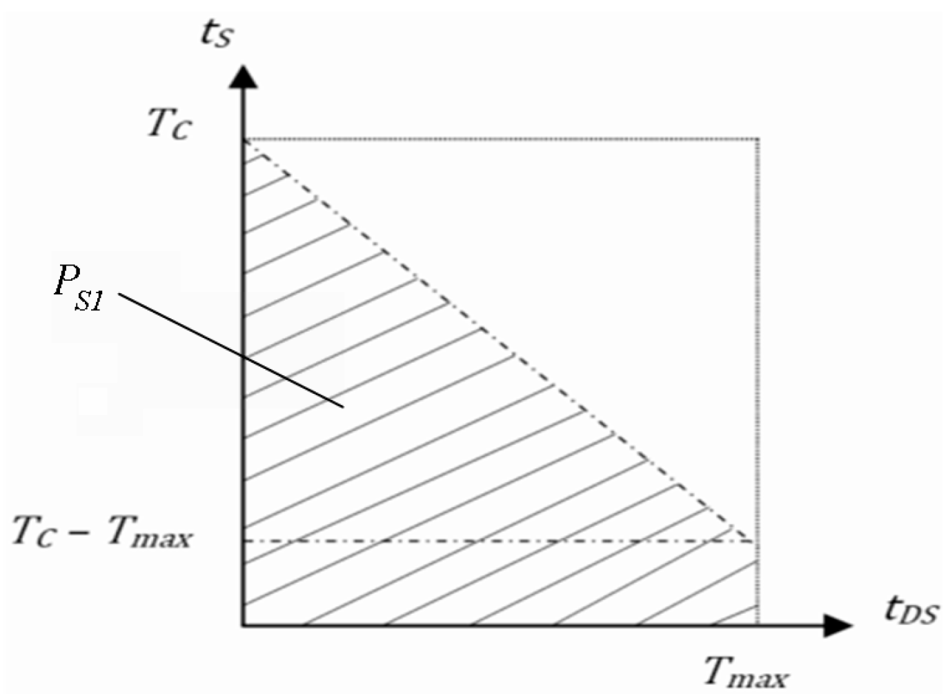
It is assumed that $t_S$ is uniformly distributed over the segment [0, $T_C$) and $t_{DS}$ is uniformly distributed over the segment [0, $T_{\max }$). The zero value of $t_{DS}$ corresponds to the SE in the stage’s CP output cascade cell. In accordance with the hypothesis of fault source flow density immutability, the SE is written to the register if the following conditions are simultaneously met:

$$\left\{\begin{array}{l}{T}_{SE}>T_C-\left(t_S+t_{DS}\right),\\ t_S+t_{DS}<T_C.\end{array}\right.$$

The probability $P_{S1}$ of the condition ($t_S+t_{DS}<T_C$) being fulfilled is estimated using the geometric method illustrated in Figure 3. It is expressed by the following formula:

$$P_{S1}={\displaystyle \frac{0.5T_{\max }{}^2+T_{\max }\left(T_C-T_{\max }\right)}{T_C{T}_{\max }}}=1-{\displaystyle \frac{T_{\max }}{2T_C}}=1-0.5k_P.$$

It is a constant with fixed clock frequency values, supply voltage, and ambient temperature.

Then, an SE that hit the stage’s CP enters the stage register with a probability whose integral function $F_{CP\_S}$ is described by the following formula:

$$F_{CP\_S}\left(t_S,t_{DS}\right)={\displaystyle \frac{(1-0.5k_P)P_{NM}}{K_{err}}}\left(1-{\displaystyle \frac{1}{{\sigma }_{SE}\sqrt{2\pi }}}{\displaystyle \underset{0}{\overset{T_C-\left(t_S+t_{DS}\right)}{\int }}{e}^{-\frac{{\left(x-m_{SE}\right)}^2}{2{\sigma }_{SE}^2}}dx}\right).$$

(3)

The SE can hit the pipeline stage register. Taking into account the typical register bit circuit design as a D-flip–flop on bidirectional keys and inverters, the SE’s uniform distribution in time and the independence of the SE’s appearance in different nets of the register bit circuit, the integral function $F_{R\_S}$ of the probability of the critical SE’s appearance in it is estimated using the following formula:

$$F_{R\_S}(t_S)={\displaystyle \frac{1}{16}}\left\{{\displaystyle \frac{5}{K_{err}}}+5-{\displaystyle \frac{1}{K_{err}{\sigma }_{SE}\sqrt{2\pi }}}\left[3{\displaystyle \underset{0}{\overset{T_C-t_S}{\int }}{e}^{-\frac{{\left(x-m_{SE}\right)}^2}{2{\sigma }_{SE}^2}}dx}+2{\displaystyle \underset{0}{\overset{t_I}{\int }}{e}^{-\frac{{\left(x-m_{SE}\right)}^2}{2{\sigma }_{SE}^2}}dx}\right]\right\},$$

(4)

where $t_I$ is the inverter switching delay.

In accordance with the hypothesis that only a single SE can be observed at any time, the events leading to the appearance of an SE in the CP or in the stage register are incompatible. The probability of a nuclear particle entering the CP or stage register area is directly proportional to the die area of the CP ($S_{CP\_S}$) and the register ($S_{R\_S}$). Then, the critical SE’s total probability in a synchronous pipeline stage can be described by the integral probability function $F_{CF\_S}$:

$$\begin{array}{l}{F}_{CF\_S}(t_S,t_{DS})={\displaystyle \frac{S_{CP\_S}}{\left(S_{CP\_S}+S_{R\_S}\right)}}{\displaystyle \frac{(1-0.5k_P)P_{NM}}{K_{err}}}\left[1-{\displaystyle \frac{1}{{\sigma }_{SE}\sqrt{2\pi }}}{\displaystyle \underset{0}{\overset{T_C-t_S-t_{DS}}{\int }}{e}^{-\frac{{\left(x-m_{SE}\right)}^2}{2{\sigma }_{SE}^2}}dx}\right]+\\ +{\displaystyle \frac{S_{R\_S}}{16\left(S_{CP\_S}+S_{R\_S}\right)}}\left\{{\displaystyle \frac{5}{K_{err}}}+5-{\displaystyle \frac{1}{K_{err}{\sigma }_{SE}\sqrt{2\pi }}}\left[3{\displaystyle \underset{0}{\overset{T_C-t_S}{\int }}{e}^{-\frac{{\left(x-m_{SE}\right)}^2}{2{\sigma }_{SE}^2}}dx}+2{\displaystyle \underset{0}{\overset{t_I}{\int }}{e}^{-\frac{{\left(x-m_{SE}\right)}^2}{2{\sigma }_{SE}^2}}dx}\right]\right\}.\end{array}$$

(5)

Let us introduce the Laplace integral function Φ(x) [43] into Equation (5) by substitution:

$${\displaystyle \frac{x-m_{SE}}{{\sigma }_{SE}}}=u;dx={\sigma }_{SE}du.$$

(6)

Then, Equation (5) changes to the formula:

$$\begin{array}{l}{F}_{CF\_S}\left(t_S,t_{DS}\right)={\displaystyle \frac{\left(1-0.5k_P\right)P_{NM}{S}_{CP\_S}}{K_{err}\left(S_{CP\_S}+S_{R\_S}\right)}}\left[1-\mathsf{\Phi }\left({\displaystyle \frac{T_C-t_S-t_{DS}-m_{SE}}{{\sigma }_{SE}}}\right)-\mathsf{\Phi }\left({\displaystyle \frac{m_{SE}}{{\sigma }_{SE}}}\right)\right]+\\ +{\displaystyle \frac{S_{R\_S}}{16\left(S_{CP\_S}+S_{R\_S}\right)}}\left\{{\displaystyle \frac{5}{K_{err}}}+5-{\displaystyle \frac{1}{K_{err}}}\left[3\mathsf{\Phi }\left({\displaystyle \frac{T_C-t_S-m_{SE}}{{\sigma }_{SE}}}\right)+5\mathsf{\Phi }\left({\displaystyle \frac{m_{SE}}{{\sigma }_{SE}}}\right)+2\mathsf{\Phi }\left({\displaystyle \frac{t_I-m_{SE}}{{\sigma }_{SE}}}\right)\right]\right\}.\end{array}$$

(7)

Formula (7) serves as a mathematical stochastic model of a critical SE in a synchronous pipeline stage caused by the impact of a nuclear particle running through the chip body. It has been obtained for the case of nuclear particle flow leading to the appearance of a single SE and allows one to estimate the probability of a critical SE depending on the SE’s parameters, appearance, place, and time.

5. Critical Soft Errors in the Self-Timed Pipeline Stage

Self-timed circuits use redundant data encoding. Combinational ST circuits typically use dual-rail (DR) encoding with a spacer. The DR signal has two working states (“01” and “10”) and one spacer state (“00” or “11”). The DR signal can switch into an antispacer state, opposite to the spacer, only under the influence of an SE. With a proper ST circuit layout design [30,44], the DR signal fault manifests itself as one of the following events:

• A working state instead of a spacer;
• A spacer instead of a working state;
• An antispacer instead of a spacer;
• An antispacer instead of a working state.

For simplicity, we assume that adjacent ST pipeline stages are well matched and have approximately the same performance. Let us introduce the set of variables we operate with to estimate the probability of an SE in ST circuits, which is presented in

Table 2. Variables for calculating SE probability in self-timed circuits.

Variable	Name
An SE’s appearance time relative to the interval Ii beginning	$t_i$, i = 1…4
Interval Ii duration	$T_i$, i = 1…4
Faulty DR signal switching to the expected state	$t_{DR}$
Inclusive OR cell’s switching delay	$t_{NX}$
C-element switching delay	$t_{CE}$
Die area of the stage’s CP	$S_{CP\_ST}$
Die area of the stage’s register	$S_{R\_ST}$
Die area of the entire ST pipeline stage	$S_{A\_ST}$

. This probability also depends on the following factors:

• A faulty subcircuit (stage CP or register);
• Correspondence of the DR signal’s faulty state to the expected state in the current phase;
• The probability of writing a faulty DR signal into the stage register.

Assume that the occurrence time $t_i$, i = 1…4, is uniformly distributed over the interval [0, $T_i$), i = 1…4, and the time $t_{DR}$ is uniformly distributed over the interval [0, $T_j$), j = {1; 3}. The $t_{DR}$ and $t_{NX}$ have fixed values under the given operating conditions.

In an ST pipeline, the probability that an SE that hit a pipeline stage becomes critical depends not only on the hit stage’s response to the SE but also on its neighbors. In particular, maintaining the state of the current stage inputs during the SE action depends on the stage’s indication subcircuit and the previous stage’s register. Writing a faulty DR signal to the register of the current stage depends on the subsequent stage.

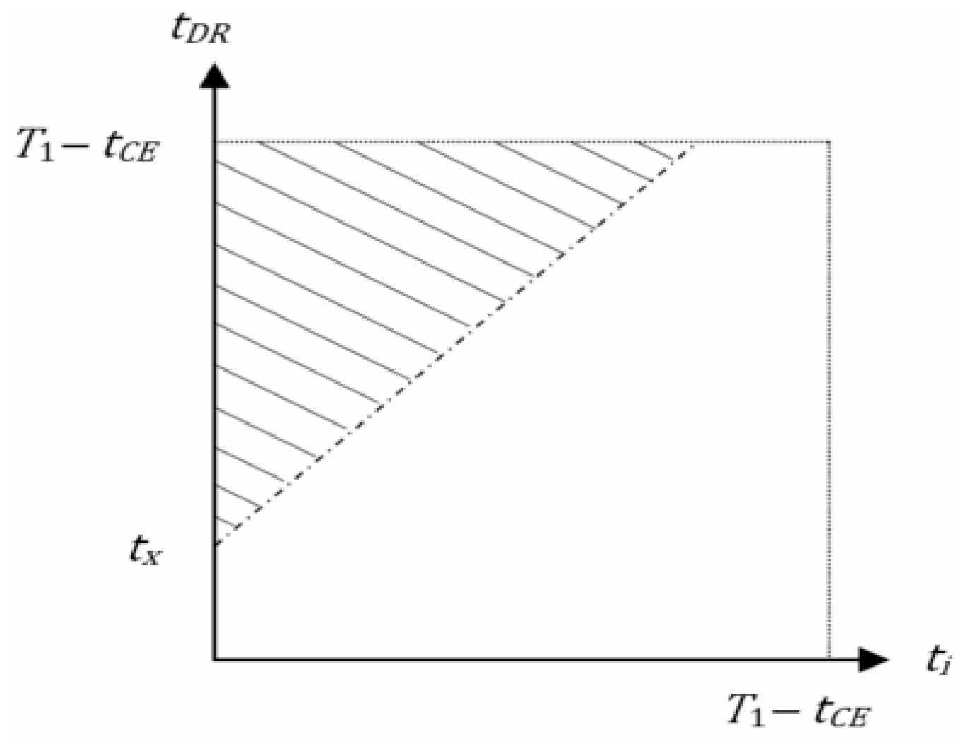
An SE, affecting the DR signal component in the ST pipeline stage’s CP, can become critical only if the following conditions are simultaneously met:

$$\left\{\begin{array}{l}{t}_{CE}\le t_{DR}+t_i,i=\left\{1;3\right\},\\ t_{NX}\le t_{DR}+t_i,i=\left\{1;3\right\}.\end{array}\right.$$

(8)

The probability of fulfilling each of the conditions in Equation (8) is estimated using the geometric method illustrated in Figure 4 for the SE at interval I₁. Here, $t_x$ denotes $t_{CE}$ or $t_{NX}$.

Let the ST pipeline stage CP and register indication subcircuits be implemented on three-input C-elements. The C-element masks the premature switching of one of its inputs in 75% of cases. Then, the probability function $F_C$ of the C-element indicating a faulty DR signal prematurely switching to the expected state due to the SE is determined by the formula:

$$F_C(T_1)={\displaystyle \frac{{\left(T_1-2t_{CE}\right)}^2{\left(T_1-t_{CE}-t_{NX}\right)}^2}{4{\left(T_1-t_{CE}\right)}^4}},$$

(9)

Taking into account the request–acknowledge interaction of the ST pipeline stages and the CP and register die areas, the integral function $F_{T1}$ of the probability of the critical SE’s occurrence in the ST pipeline stage at interval I₁ equals:

$$F_{T1}(T_1,T_2)={\displaystyle \frac{P_{NM}{}^{2}F_C{(T_1)}^2{\left(T_1-2t_{CE}\right)}^2\left(3S_{CP\_ST}+S_{R\_ST}\right)}{128{\left(T_1-t_{CE}\right)}^2{S}_{A\_ST}{K}_{err}}}\left(1-{\displaystyle \frac{1}{{\sigma }_{SE}\sqrt{2\pi }}}{\displaystyle \underset{0}{\overset{T_1+T_2-t_{CE}}{\int }}{e}^{-\frac{{\left(x-m_{SE}\right)}^2}{2{\sigma }_{SE}^2}}dx}\right),$$

Note that $S_{CP\_ST}$ and $S_{R\_ST}$ do not take into account the indication subcircuit areas of the CP and register, since an SE’s appearance in the indication subcircuit at interval I₁ is not critical.

At interval I₂, the outputs of this stage have already switched to the working state and initiated the subsequent stage transition to the working phase. Depending on the SE’s appearance time $t_2$ and the place of its impact, it becomes critical with a probability described by the integral function $F_{T2}$:

$$\begin{array}{l}{F}_{T2}(T_1,T_2,T_3,t_{DR},t_2)={\displaystyle \frac{P_{NM}{}^{2}S_{CP\_ST}}{2S_{A\_ST}{K}_{err}}}\left(1-{\displaystyle \frac{1}{{\sigma }_{SE}\sqrt{2\pi }}}{\displaystyle \underset{0}{\overset{T_1+T_2+t_{CE}-t_2}{\int }}{e}^{-\frac{{\left(x-m_{SE}\right)}^2}{2{\sigma }_{SE}^2}}dx}\right)+\\ +{\displaystyle \frac{P_{NM}\left(T_2-t_{NX}\right)\left(T_2-t_{CE}\right)S_{R\_ST}}{2T_2{}^{2}S_{A\_ST}{K}_{err}}}\left(1-{\displaystyle \frac{1}{{\sigma }_{SE}\sqrt{2\pi }}}{\displaystyle \underset{0}{\overset{T_2+T_3+t_{CE}-t_2}{\int }}{e}^{-\frac{{\left(x-m_{SE}\right)}^2}{2{\sigma }_{SE}^2}}dx}\right),\end{array}$$

Interval I₃ combines the time of the current stage’s CP outputs switching to the spacer and the time of writing the spacer onto the current stage register. Depending on the SE’s appearance time $t_3$ and the place of its impact, it becomes critical with a probability described by the integral function $F_{T3}$:

$$\begin{array}{l}{F}_{T3}(T_1,T_3,t_{DR},t_3)={\displaystyle \frac{3P_{NM}{}^2\left(2T_3-T_1-t_{CE}\right)^2{S}_{CP\_ST}}{8T_3{S}_{A\_ST}{K}_{err}}}\left(1-{\displaystyle \frac{1}{{\sigma }_{SE}\sqrt{2\pi }}}{\displaystyle \underset{0}{\overset{T_3+t_{CE}-t_{DR}}{\int }}{e}^{-\frac{{\left(x-m_{SE}\right)}^2}{2{\sigma }_{SE}^2}}dx}\right)+\\ +{\displaystyle \frac{P_{NM}{S}_{R\_ST}{T}_3}{2S_{A\_ST}{K}_{err}}}\left(1-{\displaystyle \frac{1}{{\sigma }_{SE}\sqrt{2\pi }}}{\displaystyle \underset{0}{\overset{T_1+t_{CE}-t_3}{\int }}{e}^{-\frac{{\left(x-m_{SE}\right)}^2}{2{\sigma }_{SE}^2}}dx}\right).\end{array}$$

An analysis of possible outcomes when an SE occurs at interval I₄ shows that none of them lead to a critical SE. In the worst case, they only cause a temporary suspension of the pipeline operation.

The events of a single SE occurrence in different ST pipeline cycle intervals are incompatible. Therefore, the total integral function of the probability of a critical SE occurrence in the ST pipeline stage equals the sum of the probability of an SE occurrence at individual intervals, weighted by the ratio of their durations to the total duration of all intervals:

$$\begin{array}{l}{F}_{CF\_ST}(T_1,T_2,T_3,t_{DR},t_2,t_3)={\displaystyle \frac{F_{T1}(T_1,T_2)T_1+F_{T2}(T_1,T_2,T_3,t_{DR},t_2)T_2+F_{T3}(T_1,T_3,t_{DR},t_3)T_3}{T_1+T_2+T_3+T_4}}=\\ =\left[{\displaystyle \frac{P_{NM}{}^{2}F_C{\left(T_1\right)}^2{\left(T_1-2t_{CE}\right)}^2\left(3S_{CP\_ST}+S_{R\_ST}\right)T_1}{128{\left(T_1-t_{CE}\right)}^2{S}_{A\_ST}{K}_{err}}}\left(1-{\displaystyle \frac{1}{{\sigma }_{SE}\sqrt{2\pi }}}{\displaystyle \underset{0}{\overset{T_1+T_2+t_{CE}}{\int }}{e}^{-\frac{{\left(x-m_{SE}\right)}^2}{2{\sigma }_{SE}^2}}dx}\right)+\right.\\ +{\displaystyle \frac{P_{NM}{}^{2}S_{CP\_ST}{T}_2}{2S_{A\_ST}{K}_{err}}}\left(1-{\displaystyle \frac{1}{{\sigma }_{SE}\sqrt{2\pi }}}{\displaystyle \underset{0}{\overset{T_1+T_2+t_{CE}+t_{DR}-t_2}{\int }}{e}^{-\frac{{\left(x-m_{SE}\right)}^2}{2{\sigma }_{SE}^2}}dx}\right)+\\ +{\displaystyle \frac{P_{NM}\left(T_2-t_{NX}\right)\left(T_2-t_{CE}\right)S_{R\_ST}}{2T_2{S}_{A\_ST}{K}_{err}}}\left(1-{\displaystyle \frac{1}{{\sigma }_{SE}\sqrt{2\pi }}}{\displaystyle \underset{0}{\overset{T_2+T_3+t_{CE}-t_2}{\int }}{e}^{-\frac{{\left(x-m_{SE}\right)}^2}{2{\sigma }_{SE}^2}}dx}\right)+\\ +{\displaystyle \frac{3P_{NM}{}^2\left(2T_3-T_1-t_{CE}\right)^2{S}_{CP\_ST}}{8T_3{S}_{A\_ST}{K}_{err}}}\left(1-{\displaystyle \frac{1}{{\sigma }_{SE}\sqrt{2\pi }}}{\displaystyle \underset{0}{\overset{T_3+t_{CE}-t_{DR}}{\int }}{e}^{-\frac{{\left(x-m_{SE}\right)}^2}{2{\sigma }_{SE}^2}}dx}\right)+\\ \left. +{\displaystyle \frac{P_{NM}{S}_{R\_ST}{T}_3}{2S_{A\_ST}{K}_{err}}}\left(1-{\displaystyle \frac{1}{{\sigma }_{SE}\sqrt{2\pi }}}{\displaystyle \underset{0}{\overset{T_1+t_{CE}-t_3}{\int }}{e}^{-\frac{{\left(x-m_{SE}\right)}^2}{2{\sigma }_{SE}^2}}dx}\right)\right]{\displaystyle \frac{1}{\left(T_1+T_2+T_3+T_4\right)}},\end{array}$$

(10)

After moving to the Laplace integral function using the substituted Equations (6) and (9), we obtain:

$$\begin{array}{l}{F}_{CF\_ST}(T_1,T_2,T_3,t_2,t_3,t_{DR})=\left\{{\displaystyle \frac{P_{NM}{}^2\left(T_1-t_{CE}-t_{NX}\right)^4{\left(T_1-2t_{CE}\right)}^6\left(3S_{CP\_ST}+S_{R\_ST}\right)}{2048{\left(T_1-t_{CE}\right)}^{10}{S}_{A\_ST}}}\left[1-\right.\right.\\ -\mathsf{\Phi }\left({\displaystyle \frac{T_1+T_2+t_{CE}-m_{SE}}{{\sigma }_{SE}}}\right)\left.-\mathsf{\Phi }\left({\displaystyle \frac{m_{SE}}{{\sigma }_{SE}}}\right)\right]T_1+\left({\displaystyle \frac{P_{NM}^2}{2}}\left[1-\mathsf{\Phi }\left({\displaystyle \frac{T_1+T_2+t_{CE}+t_{DR}-t_2-m_{SE}}{{\sigma }_{SE}}}\right)-\mathsf{\Phi }\left({\displaystyle \frac{m_{SE}}{{\sigma }_{SE}}}\right)\right]+\right.\\ \left.+{\displaystyle \frac{P_{NM}\left(T_2-t_{CE}\right)\left(T_2-t_{NX}\right)}{2T_2^2}}\left[1-\mathsf{\Phi }\left({\displaystyle \frac{T_3+T_2+t_{CE}-t_2-m_{SE}}{{\sigma }_{SE}}}\right)-\mathsf{\Phi }\left({\displaystyle \frac{m_{SE}}{{\sigma }_{SE}}}\right)\right]\right){\displaystyle \frac{S_{CP\_ST}}{S_{A\_ST}}}{T}_2+\\ +\left({\displaystyle \frac{3P_{NM}{}^2\left(2T_3-T_1-t_{CE}\right)^2}{8T_3^2}}\left[1-\mathsf{\Phi }\left({\displaystyle \frac{T_3+t_{CE}-t_{DR}-m_{SE}}{{\sigma }_{SE}}}\right)-\mathsf{\Phi }\left({\displaystyle \frac{m_{SE}}{{\sigma }_{SE}}}\right)\right]+\right.\\ +\left.\left.{\displaystyle \frac{P_{NM}}{2}}\left[1-\mathsf{\Phi }\left({\displaystyle \frac{T_1+t_{CE}-t_3-m_{SE}}{{\sigma }_{SE}}}\right)-\mathsf{\Phi }\left({\displaystyle \frac{m_{SE}}{{\sigma }_{SE}}}\right)\right]\right){\displaystyle \frac{S_{R\_ST}}{S_{A\_ST}}}{T}_3\right\}{\displaystyle \frac{1}{K_{err}\left(T_1+T_2+T_3+T_4\right)}}.\end{array}$$

(11)

Formula (11) serves as a mathematical probability model of a critical SE caused by a nuclear particle in the ST pipeline stage. It can be divided into two components that determine the probability of a critical SE in the stage CP ($F_{CP\_ST}$) and register ($F_{R\_ST}$):

$$\begin{array}{l}{F}_{CP\_ST}(T_1,T_2,T_3,t_2,t_{DR})=\left\{{\displaystyle \frac{3{\left(T_1-t_{CE}-t_{NX}\right)}^4{\left(T_1-2t_{CE}\right)}^6}{1024{\left(T_1-t_{CE}\right)}^{10}}}\left[1-\mathsf{\Phi }\left({\displaystyle \frac{T_1+T_2+t_{CE}-m_{SE}}{{\sigma }_{SE}}}\right)-\right.\right.\left.\mathsf{\Phi }\left({\displaystyle \frac{m_{SE}}{{\sigma }_{SE}}}\right)\right]T_1+\\ +\left[1-\mathsf{\Phi }\left({\displaystyle \frac{T_1+T_2+t_{CE}+t_{DR}-t_2-m_{SE}}{{\sigma }_{SE}}}\right)-\mathsf{\Phi }\left({\displaystyle \frac{m_{SE}}{{\sigma }_{SE}}}\right)\right]T_2+\\ \left.+{\displaystyle \frac{3{\left(2T_3-T_1-t_{CE}\right)}^2}{4T_3^2}}\left[1-\mathsf{\Phi }\left({\displaystyle \frac{T_3+t_{CE}-t_{DR}-m_{SE}}{{\sigma }_{SE}}}\right)-\mathsf{\Phi }\left({\displaystyle \frac{m_{SE}}{{\sigma }_{SE}}}\right)\right]T_3\right\}{\displaystyle \frac{S_{CP\_ST}{P}_{NM}^2}{2S_{A\_ST}{K}_{err}\left(T_1+T_2+T_3+T_4\right)}},\end{array}$$

(12)

$$\begin{array}{l}{F}_{R\_ST}(T_1,T_2,T_3,t_2,t_3)=\left\{{\displaystyle \frac{P_{NM}{\left(T_1-t_{CE}-t_{NX}\right)}^4{\left(T_1-2t_{CE}\right)}^6}{1024{\left(T_1-t_{CE}\right)}^{10}}}\left[1-\mathsf{\Phi }\left({\displaystyle \frac{T_1+T_2+t_{CE}-m_{SE}}{{\sigma }_{SE}}}\right)-\right.\right.\\ \left. -\mathsf{\Phi }\left({\displaystyle \frac{m_{SE}}{{\sigma }_{SE}}}\right)\right]T_1+{\displaystyle \frac{\left(T_2-t_{CE}\right)\left(T_2-t_{NX}\right)}{T_2^2}}\left[1-\mathsf{\Phi }\left({\displaystyle \frac{T_3+T_2+t_{CE}-t_2-m_{SE}}{{\sigma }_{SE}}}\right)-\mathsf{\Phi }\left({\displaystyle \frac{m_{SE}}{{\sigma }_{SE}}}\right)\right]T_2+\\ +\left.\left[1-\mathsf{\Phi }\left({\displaystyle \frac{T_1+t_{CE}-t_3-m_{SE}}{{\sigma }_{SE}}}\right)-\mathsf{\Phi }\left({\displaystyle \frac{m_{SE}}{{\sigma }_{SE}}}\right)\right]T_3\right\}{\displaystyle \frac{P_{NM}{S}_{R\_ST}}{2S_{A\_ST}{K}_{err}\left(T_1+T_2+T_3+T_4\right)}}.\end{array}$$

(13)

Formulas (12) and (13) serve as mathematical stochastic models of the critical SE caused by a nuclear particle in the ST pipeline stage CP and register, respectively.

6. Critical Soft Errors in a Pipeline

The probability of a critical SE in the pipeline, generated by a single SE, depends on the probability of its occurrence in one stage and the affected stage’s location in the pipeline structure. In a typical pipeline consisting of N stages, a critical SE in the k-th stage (k = 1, …, N–1) can be masked by the subsequent stage logics. Then, the probability of the occurrence of a critical SE in the entire pipeline output when a single SE impacts one of its stages is described by the integral function:

$$F_{CF\_P}={\displaystyle \frac{1}{N}}{\displaystyle \sum _{k=1}^N\left(P_{NM}{}^{N-k}F_{CF,k}\right)},$$

(14)

where $F_{CF,k}$ is the integral function of the critical SE probability in the k-th pipeline stage. Formula (14) is invariant to the synchronous and ST pipelines.

7. Discussion

Formulas (3)–(5), (7) and (10)–(14) correspond to the mathematical model definition: “A mathematical model is an approximate description of some class of phenomena, objects of the external world, expressed by means of mathematical concepts and symbols” [45]. Indeed, they describe the critical SE phenomenon in the synchronous and ST pipeline stage by means of mathematical concepts and symbols within the framework of formulated hypotheses and depending on some variables:

• Random time variables ($t_S,t_i$, i = 1…4, $t_{DS},t_{DR}$), uniformly distributed over the corresponding intervals.
• SE durations distributed according to a truncated normal law.
• Logical cell transition delays that take a constant value at a given supply voltage and temperature.
• The duration of the clock period (in a synchronous pipeline) or an operation phase (in an ST pipeline).

These critical SE mathematical models are stochastic. They represent the probability that an SE appearing in the pipeline stage due to the impact of a nuclear particle running through the chip body becomes critical, i.e., corrupts data processing results or stops the pipeline’s operation. Substituting the SEs’ physical parameters and the specific values of their variables corresponding to the specified operating conditions and manufacturing technology process into these functions allows one to obtain the critical SE probability’s numerical value in the pipeline stage and compare the fault tolerance levels of the synchronous and ST pipeline stages.

For the synchronous pipeline stage, such random variables are $t_S$ and $t_{DS}$, which are distributed uniformly over the intervals (0, $T_C$) and (0, $T_{\max }$], respectively, and characterize the time and place of the SE’s appearance in the pipeline stage. The remaining variables in Formulas (3)–(5) and (7) have fixed values for a specific pipeline circuit, a given synchronization frequency, supply voltage, and ambient temperature.

For the ST pipeline stage, the random variables in Formulas (10)–(13) are $T_1,T_2,T_3,t_2,t_3$, and $t_{DR}$. The first three of them depend mainly on the ST pipeline stage’s complexity, supply voltage, and ambient temperature. The random variables $t_2,t_3$, and $t_{DR}$ characterize the time of the SE’s appearance and its place in the pipeline stage. Input data also introduce some randomness to Formulas (10)–(13), as their values affect the time of their processing in the ST pipeline stage.

For example, let us carry out a specific numerical calculation using the obtained models. To obtain quantitative estimates of the fault tolerance level of the synchronous and ST pipeline stages, we substitute typical values of the parameters used in them, which are characteristic of the 65 nm CMOS process, into Equations (7) and (11): $P_{NM}$ = 0.9; $T_C$ = 1 ns; $k_P$ = 0.8; $S_{CP\_S}$ = 0.8$\left(S_{CP\_S}+S_{CP\_S}\right)$; $t_{CE}$ = 40 ps; $t_{NX}$ = 20 ps; $t_I$ = 5 ps; $S_{CP\_ST}$ = 0.6$S_{A\_ST}$; $S_{R\_ST}$ = 0.12$S_{A\_ST}$. The normalizing coefficient $K_{err}$ is determined by Equation (2) using the Laplace integral function for the selected parameters of the SE’s duration and probability distribution function:

$$K_{err}=1-\left(\mathsf{\Phi }\left(-{\displaystyle \frac{m_{SE}}{{\sigma }_{SE}}}\right)-\mathsf{\Phi }(-\infty )\right)=0.5+\mathsf{\Phi }\left({\displaystyle \frac{m_{SE}}{{\sigma }_{SE}}}\right).$$

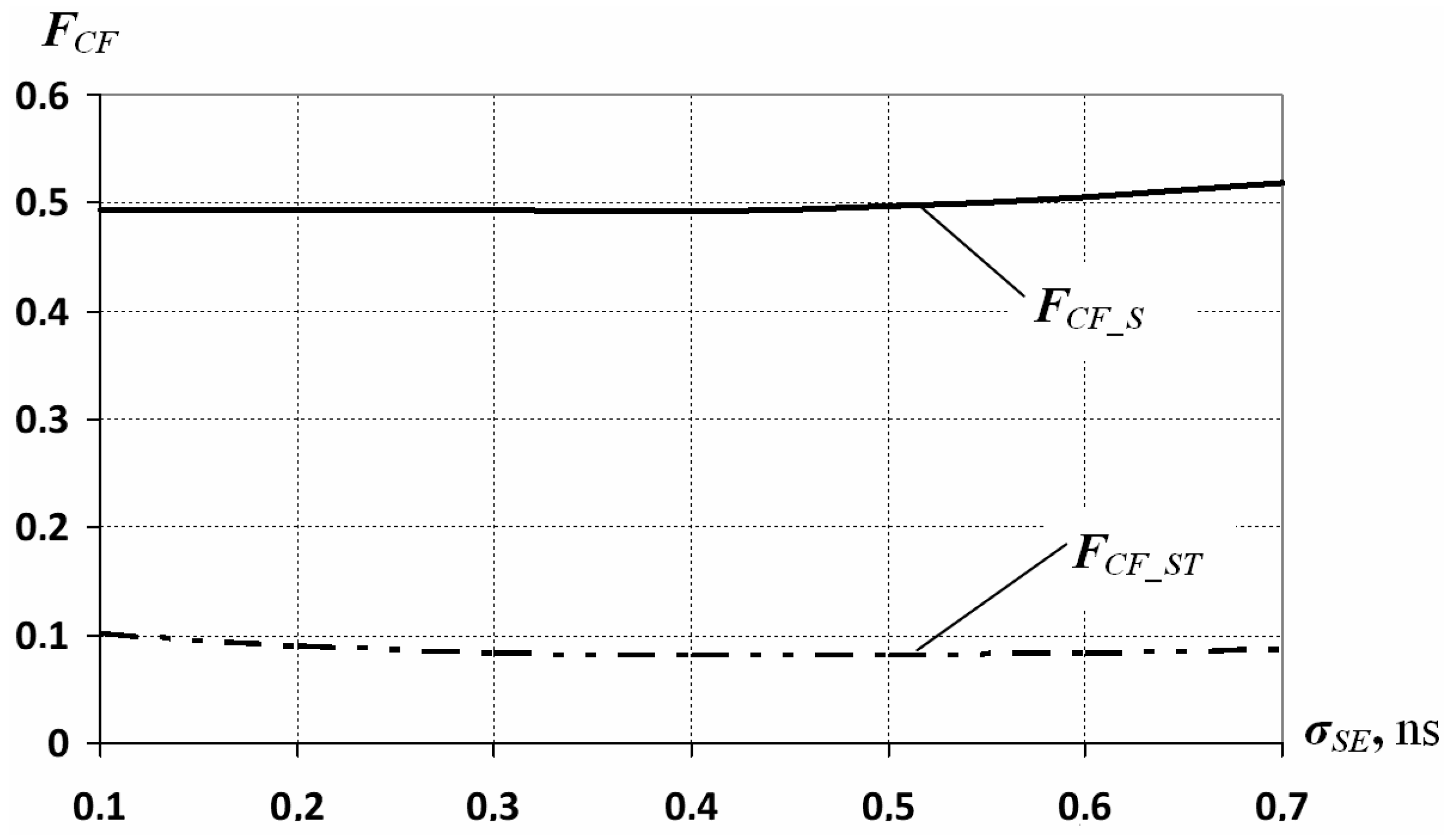
Figure 5 shows dependence diagrams for the probability of the occurrence of the critical SE integral functions $F_{CF\_S}$ and $F_{CF\_ST}$ on the variance in the SE duration distribution function ${\sigma }_{SE}$ with the mathematical expectation $m_{SE}$ = 1 ns calculated from Equations (7) and (11) for typical values of $t_S$ = 0.5 ns, $t_{DS}$ = 0.4 ns, $T_1=T_3$ = 0.5 ns, $T_2$ = 0.3 ns, $t_2$ = 0.15 ns, $t_3$ = 0.25 ns, $t_{DR}$ = 0.23 ns. Figure 6 shows dependence diagrams for the functions $F_{CF\_S}$ and $F_{CF\_ST}$ on the mathematical expectation $m_{SE}$ with the variance ${\sigma }_{SE}$ = 0.4 ns and the same typical values for the other variables in Equations (7) and (11).

Figure 5 shows that for the specific values of the mathematical expectation $m_{SE}$ = 1 ns and variance ${\sigma }_{SE}$ = 0.4 ns for the SE duration distribution, the probabilities of the critical SE occurrence in the synchronous ($P_{CF\_S}$) and ST pipeline ($P_{CF\_ST}$) stages equal $P_{CF\_S}$ = 0.493 and $P_{CF\_ST}$ = 0.081. The ratio of $P_{CF\_S}$ and $P_{CF\_ST}$ shows that an ST pipeline stage is 6.1 times better protected from an SE than the synchronous pipeline stage.

For eight-stage synchronous and ST pipelines (N = 8), where all stages are matched in hardware complexity and speed, with the above variable values, the critical SE probability estimates according to Equation (14) are 0.350 for the synchronous pipeline and 0.057 for the ST pipeline. The advantage of the ST pipeline over the synchronous counterpart remained at the same level.

Thus, the mathematical models obtained allow one to estimate the SE tolerance level of the synchronous and ST pipelines. The resulting quantitative estimates of the critical SE probabilities in the synchronous and ST pipelines using these models support the qualitative result obtained in [30,40,41]. Further research will be devoted to the construction of a mathematical model of multiple SEs in synchronous and ST circuits.

8. Conclusions

Self-timed circuits are hardware-redundant and require proportionally more die area on the chip. Because of this, they are more susceptible to the influence of SEs compared to their synchronous counterparts. At a constant density of nuclear particle flux affecting the circuit, the intensity of an SE in an ST pipeline is also proportionally greater. However, due to the two-phase discipline and redundant data coding and dual rails in combinational circuits and pipeline registers, the ST pipeline masks SEs much better than its synchronous counterpart.

The stochastic mathematical models obtained describe the phenomenon of a single critical SE in a synchronous and ST pipeline. They allow one to evaluate and compare the stability levels of synchronous and ST pipelines to the SE source’s impact in the case when the SE duration is distributed according to the normal law and the flow density of the SE sources is uniformly distributed in time and over the chip area.

Quantitative estimates of the synchronous and ST pipeline stages’ SE immunity are obtained for integrated circuit components with typical operating conditions and electrical parameters. They are based on the mathematical models developed and prove the ST pipeline’s advantage in terms of SE tolerance over its synchronous counterpart, being 6.1 times better.

In future studies, we intend to create stochastic models of multiple soft errors in synchronous and self-timed circuits.

References

- Koons, H.C.; Mazur, J.E.; Selesnick, R.S.; Blake, J.B.; Fennell, J.F.; Roeder, J.; Anderson, P.C. The Impact of the Space Environment on Space Systems, Proceedings of the 6th Spacecraft Charging Technology, AFRL-VS-TR-20001578. 1 September 2000. pp. 7–11. Available online: https://www.researchgate.net/publication/234189291_The_Impact_of_the_Space_Environment_on_Space_Systems (accessed on 22 January 2025).
- Baumann, R.C. Radiation-Induced Soft Errors in Advanced Semiconductor Technologies. IEEE Trans. Device Mater. Reliab. 2005, 5, 305–316. [Google Scholar] [CrossRef]
- Artemov, M.E.; Khamidullina, N.M.; Kombaev, T.S.; Vlasenkov, E.V.; Zefirov, I.V.; Chernikov, P.S. Determination of requirements for radiation dose effect resistance of electronic and radio equipment of a promising spacecraft for studying main-belt asteroids. In Issues of Atomic Science and Technology. Series: Physics of Radiation Effects on Electronic Equipment; JSC “Research Institute of Instruments”: Moscow, Russia, 2020; Volume 4, pp. 35–38. (In Russian) [Google Scholar]
- Mavis, D.; Eaton, P. SEU and SET modeling and mitigation in deep submicron technologies. In Proceedings of the 2007 IEEE International Reliability Physics Symposium Proceedings. 45th Annual, Phoenix, AZ, USA, 15–19 April 2007; pp. 293–305. [Google Scholar] [CrossRef]
- Viktorova, V.S.; Lubkov, N.V.; Stepanyants, A.S. Fault-Tolerant Control Computer Systems’ Reliability Analysis; Institute of Control Problems RAS: Moscow, Russia, 2016; 117p, Available online: https://www.ipu.ru/sites/default/files/card_file/VLS.pdf (accessed on 22 January 2025). (In Russian)
- Shubinsky, I.B. Functional Reliability of Information Systems. Analysis Methods; Journal Reliability: Moscow, Russia, 2012; 296p, Available online: https://www.dependability.ru/jour/manager/files/books/Книга.pdf (accessed on 22 January 2025). (In Russian)
- White, A.L. Establishing Fault Tolerance for a Class of Systems by Experiment. Available online: https://ntrs.nasa.gov/api/citations/20210013688/downloads/NASA-TM-20210013688.pdf (accessed on 22 January 2025).
- Aneesh, Y.M.; Bindu, B.A. Physics-Based Single Event Transient Pulse Width Model for CMOS VLSI Circuits. IEEE Trans. Device Mater. Reliab. 2020, 20, 723–730. [Google Scholar] [CrossRef]
- Cai, S.; He, B.; Wang, W.; Liu, P.; Yu, F.; Yin, L. Soft Error Reliability Evaluation of Nanoscale Logic Circuits in the Presence of Multiple Transient Faults. J. Electron. Test. 2020, 36, 469–483. [Google Scholar] [CrossRef]
- Selahattin, S. Soft Error Mechanisms, Modeling and Mitigation; Springer: Berlin/Heidelberg, Germany, 2016; 116p. [Google Scholar] [CrossRef]
- Venkatesha, S.; Parthasarathi, R. A Survey of Fault Mitigation Techniques for Multi-Core Architectures. 2020; 21p. Available online: https://arxiv.org/pdf/2112.14952v1 (accessed on 22 January 2025).
- Ghavami, B.; Raji, M. Soft Error Reliability of VLSI Circuits: Analysis and Mitigation Techniques; Springer: Berlin/Heidelberg, Germany, 2021; 188p. [Google Scholar] [CrossRef]
- Sen, P.; Sadi, M.S.; Ashab, N.; Rossi, D. A New Error Correcting Coding Technique to Tolerate Soft Errors. In Proceedings of the 2021 International Conference on Electronics, Communications and Information Technology (ICECIT), Khulna, Bangladesh, 14–16 September 2021; pp. 1–4. [Google Scholar] [CrossRef]
- Khan, M.M.R.; Sadi, M.S.; Al-Zihadi, S.M.; Saha, J. Tolerating Soft Errors using Enhanced Matrix Code. In Proceedings of the 2021 International Conference on Information and Communication Technology for Sustainable Development (ICICT4SD), Dhaka, Bangladesh, 27–28 February 2021; pp. 351–355. [Google Scholar] [CrossRef]
- Stempkovsky, A.L.; Telpukhov, D.V.; Zhukova, T.D.; Gurov, S.I.; Soloviev, R.A. Methods for synthesis of fault-tolerant combinational CMOS circuits providing automatic error correction. Bull. SFedU. Eng. Sci. 2017, 7, 197–210. (In Russian) [Google Scholar]
- Tsoumanis, P.; Paliaroutis, G.-I.; Evmorfopoulos, N.; Stamoulis, G. On the Impact of Electrical Masking and Timing Analysis on Soft Error Rate Estimation in Deep Submicron Technologies. In Proceedings of the 2021 IEEE International Symposium on Defect and Fault Tolerance in VLSI and Nanotechnology Systems (DFT), Athens, Greece, 6–8 October 2021; pp. 1–6. [Google Scholar] [CrossRef]
- Hao, L.; Wang, Y.; Liu, Y.; Zhao, S.; Zhang, X.; Li, Y.; Lu, W.; Peng, C.; Zhao, Q.; Zhou, Y.; et al. Low-Cost and Highly Robust Quadruple Node Upset Tolerant Latch Design. IEEE Trans. Very Large Scale Integr. (VLSI) Syst. 2024, 32, 883–896. [Google Scholar] [CrossRef]
- Venkatesha, S.; Parthasarathi, R. 32-Bit One Instruction Core: A Low-Cost, Reliable, and Fault-Tolerant Core for Multicore Systems. J. Test. Eval. 2019, 47, 3941–3962. [Google Scholar] [CrossRef]
- Lin, D.Y.-W.; Wen, C.H.-P. DAD-FF: Hardening Designs by Delay-Adjustable D-Flip-Flop for Soft-Error-Rate Reduction. IEEE Trans. Very Large Scale Integr. (VLSI) Syst. 2020, 28, 1030–1042. [Google Scholar] [CrossRef]
- Eaton, A. Single Event Upset Immune Logic Family. U.S. Patent 6,756,809, 29 June 2004. [Google Scholar]
- Lamichhane, S.; Wang, Y.; Sayil, S. Mitigating soft errors in NCL circuits using a transmission gate. Analog. Integr. Circuits Signal Process. 2023, 115, 101–109. [Google Scholar] [CrossRef]
- Jang, W.; Martin, A. SEU-tolerant QDI circuits. In Proceedings of the 11th IEEE International Symposium on Asynchronous Circuits and Systems, New York, NY, USA, 14–16 March 2005; pp. 156–165. [Google Scholar] [CrossRef]
- Szurman, K.; Kotasek, Z. Run-Time Reconfigurable Fault Tolerant Architecture for Soft-Core Processor NEO430. In Proceedings of the 2019 IEEE 22nd International Symposium on Design and Diagnostics of Electronic Circuits & Systems (DDECS), Cluj-Napoca, Romania, 24–26 April 2019; pp. 1–4. [Google Scholar] [CrossRef]
- Dubrova, E. Fault-Tolerant Design; KTH Royal Institute of Technology: Stockholm, Sweden; Springer: Berlin/Heidelberg, Germany, 2013; 185p. [Google Scholar] [CrossRef]
- Muller, D.E.; Bartky, W.S. A theory of asynchronous circuits. In Proceedings of the International Symposium on the Theory of Switching; Harvard University Press: Cambridge, MA, USA, 1959; pp. 204–243. [Google Scholar]
- Sparsø, J. Introduction to Asynchronous Circuit Design; DTU Compute, Technical University of Denmark: Kongens Lyngby, Denmark, 2020; Available online: https://backend.orbit.dtu.dk/ws/files/215895041/JSPA_async_book_2020_PDF.pdf (accessed on 22 January 2025).
- Sparsø, J.; Staunstrup, J. Delay-insensitive multi-ring structures. Integr. VLSI J. 1993, 15, 313–340. [Google Scholar] [CrossRef]
- Varshavsky, V.; Kishinevsky, M.; Marakhovsky, V.; Peschansky, V.A.; Rosenblum, L.Y.; Taubin, A.R.; Цирлин, B. Self-Timed Control of Concurrent Processes; Kluwer Academic Publishers: Amsterdam, The Netherlands, 1990; 245p. [Google Scholar]
- Oliveira, D.L.; Verducci, O.; Torres, V.L.V.; Moreno, R.; Faria, L.A. Synthesis of QDI Combinational Circuits using Null Convention Logic Based on Basic Gates. Adv. Sci. Technol. Eng. Syst. J. 2018, 3, 308–317. [Google Scholar] [CrossRef]
- Stepchenkov, Y.A.; Kamenskih, A.N.; Diachenko, Y.G.; Rogdestvenski, Y.V.; Diachenko, D.Y. Improvement of the natural self-timed circuit tolerance to short-term soft errors. Adv. Sci. Technol. Eng. Syst. J. 2020, 5, 44–56. [Google Scholar] [CrossRef]
- Sokolov, I.A.; Stepchenkov, Y.A.; Diachenko, Y.G.; Morozov, N.V.; Stepchenkov, D.Y.; Diachenko, D.Y. Analysis of a self-timed pipeline fault tolerance. Syst. Means Inform. 2022, 32, 4–13. (In Russian) [Google Scholar] [CrossRef]
- Stepchenkov, Y.A.; Rogdestvenski, Y.V.; Shikunov, Y.I.; Diachenko, D.Y.; Diachenko, Y.G. Improvement of Self-Timed Pipeline Immunity of Soft Errors. In Proceedings of the 2021 IEEE Conference of Russian Young Researchers in Electrical and Electronic Engineering (ElConRus), St. Petersburg, Russia; Moscow, Russia, 26–29 January 2021; pp. 2045–2049. [Google Scholar] [CrossRef]
- Sokolov, I.A.; Stepchenkov, Y.A.; Diachenko, Y.G.; Rogdestvenski, Y.V.; Diachenko, D.Y. Increasing Self-Timed Circuit Soft Error Tolerance. In Proceedings of the 2020 IEEE East-West Design & Test Symposium (EWDTS), Varna, Bulgaria, 4–7 September 2020; pp. 450–454. [Google Scholar] [CrossRef]
- Danilov, I.A.; Schneider (Khazanova), A.I.; Balbekov, A.O.; Gorbunov, M.S.; Antonov, A.A. Development flow of fault-tolerant VLSI using topology-aware fault injection. In Issues of Atomic Science and Technology; Series: Physics of Radiation Effects on Radioelectronic Equipment; JSC "Research Institute of Instruments": Moscow, Russia, 2019; Volume 4, pp. 5–10. (In Russian) [Google Scholar]
- Farias, C.R.; Schvittz, R.B.; Balen, T.R.; Butzen, P.F. Evaluating Soft Error Reliability of Combinational Circuits Using a Monte Carlo Based Method. In Proceedings of the 2022 IEEE 23rd Latin American Test Symposium (LATS), Montevideo, Uruguay, 5–8 September 2022; pp. 1–6. [Google Scholar] [CrossRef]
- Balakrishnan, G.; Medeiros, C.; Gürsoy, C.C.; Hamdioui, S.; Jenihhin, M.; Alexandrescu, D. Modeling Soft-Error Reliability Under Variability. In Proceedings of the 2021 IEEE International Symposium on Defect and Fault Tolerance in VLSI and Nanotechnology Systems (DFT), Athens, Greece, 6–8 October 2021; pp. 1–6. [Google Scholar] [CrossRef]
- Gava, J.; Reis, R.; Ost, L. RAT: A Lightweight System-level Soft Error Mitigation Technique. In Proceedings of the 2020 IFIP/IEEE 28th International Conference on Very Large Scale Integration (VLSI-SOC), Salt Lake City, UT, USA, 5–7 October 2020; pp. 165–170. [Google Scholar] [CrossRef]
- Bodmann, P.R.; Papadimitriou, G.; Junior, R.L.R.; Gizopoulos, D.; Rech, P. Soft Error Effects on Arm Microprocessors: Early Estimations versus Chip Measurements. IEEE Trans. Comput. 2022, 7, 2358–2369. [Google Scholar] [CrossRef]
- Sayil, S. A survey of circuit-level soft error mitigation methodologies. Analog. Integr. Circuits Signal Process. 2019, 99, 63–70. [Google Scholar] [CrossRef]
- Sokolov, I.A.; Stepchenkov, Y.A.; Rogdestvenski, Y.V.; Diachenko, Y.G. Approximate evaluation of the effectiveness of synchronous and self-timed methodologies in problems of designing failure-tolerant computing and control systems. Autom. Remote Control. 2022, 83, 264–272. [Google Scholar] [CrossRef]
- Zatsarinny, A.A.; Stepchenkov, Y.A.; Diachenko, Y.G.; Rogdestvenski, Y.V. Failure-Tolerant Synchronous and Self-Timed Circuits Comparison. Russ. Microelectron. 2022, 51, 630–632. [Google Scholar] [CrossRef]
- Sergeev, V.O. (Ed.) Practical Training in Nuclear Physics; St. Petersburg State University: St. Petersburg, Russia, 2006; 184p. (In Russian) [Google Scholar]
- Belikova, G.I.; Vitkovskaya, L.V. Fundamentals of Probability Theory and Elements of Mathematical Statistics. Study Guide; Russian State Medical University: St. Petersburg, Russia, 2018; 160p. (In Russian) [Google Scholar]
- Balbekov, A.O.; Gorbunov, M.S.; Galimov, A.M. Design-Stage Hardening of 65-nm CMOS Standard Cells against Multiple Events. IEEE Trans. Nucl. Sci. 2021, 68, 1712–1718. [Google Scholar] [CrossRef]
- Voronenko, B.A.; Krysin, A.G.; Pelenko, V.V.; Tsuranov, O.A. Introduction to Mathematical Modeling: Training Manual; National Research University ITMO, Institute of Chemical Technology and Biotechnology: St. Petersburg, Russia, 2014; 44p. (In Russian) [Google Scholar]