Large-Eddy Simulation of the Flow Past a Circular Cylinder at Re = 130,000: Effects of Numerical Platforms and Single- and Double-Precision Arithmetic

Abstract

Numerical simulations of sub-critical flow past a circular cylinder at Reynolds number $\mathrm{R}\mathrm{e}$ = 130,000 are performed using two numerical platforms: the commercial, Ansys Fluent, and the open-source, OpenFOAM (finite volume method and large-eddy simulation based on a differential equation for the sub-grid kinetic energy). An overview of the available experimental data and similar large-eddy simulation studies is presented. A detailed analysis of all accumulated data demonstrates satisfactory agreement between them with a dispersion of approximately $20\%$ for the main integral flow parameters. A detailed comparison of the results obtained using single- and double-precision numerical methods in Ansys Fluent did not reveal any noticeable discrepancies in the integral and local flow parameters as well as the spectral characteristics. It is shown that the behavior of the dynamic system of the fluid dynamic equations computed with single precision is stable by Lyapunov and does not lead to any loss of accuracy. The reconstructed attractors of the dynamic systems in phase space are limited by an ellipsoid.

1. Introduction

The results of a large-eddy simulation (LES) of the flow over a circular cylinder for the Reynolds number $\mathrm{R}\mathrm{e}$ = 130,000 are presented. This work is a logical continuation of previous studies, where the large-eddy simulation was verified through external aerodynamic problems of various bluff bodies for the Reynolds numbers $\mathrm{R}\mathrm{e}=3900$ [1,2,3], $\mathrm{R}\mathrm{e}$ = 20,000 [4], $\mathrm{R}\mathrm{e}$ = 40,000–50,000 [5,6,7]. The present results can be used as a basis for the further development of active flow control and boundary layer separation technology using trapped vortex cells [8].

The goals and objectives are as follows:

• Further verify and validate large-eddy simulation for the turbulent separated flows at practical Reynolds numbers.
• Review the available experimental data and compare the LES results obtained by the Ansys Fluent and OpenFOAM platforms.
• Evaluate the accuracy of LES using coarse and medium-sized computational grids (10–25 million cells).
• Investigate the LES results computed with single-precision arithmetic.
• Apply stability theory and Lyapunov metrics to analyze the turbulent separated flows as dynamic systems.

The flow over a circular cylinder at different Reynolds and Mach numbers is a generally recognized benchmark in both computational and experimental aerodynamics. For the specific Reynolds number, $\mathrm{R}\mathrm{e}$ = 130,000, the pioneering LES work can be considered Breuer’s [9], which investigated numerical schemes, computational grids, and sub-grid scale models. Cao and Tamura [10] focus on the study of three-dimensional vortex structures in the wake of a cylinder by analyzing the periodicity (modulation) of time series of aerodynamic coefficients. Lloyd and James [11] test LES on fairly coarse computational grids for the Reynolds numbers $\mathrm{R}\mathrm{e}$ = 63,000–500,000. Yeon et al. [12] present detailed results from numerical simulations for several flow regimes: sub-critical ($\mathrm{R}\mathrm{e}$ = 126,000), critical ($\mathrm{R}\mathrm{e}$ = 250,000), and post-critical ($\mathrm{R}\mathrm{e}$ = 757,000). Much attention is paid to estimating the required linear size of the computational domain in the spanwise direction. For $\mathrm{R}\mathrm{e}$ = 126,000, a fairly satisfactory agreement between the predictions and experimental data was obtained. Plata et al. [13] utilize an adapted LES based on the Galerkin method for the Reynolds numbers $\mathrm{R}\mathrm{e}=3900$, $\mathrm{R}\mathrm{e}=$ = 20,000, and $\mathrm{R}\mathrm{e}=$ = 140,000.

The work of Cantwell and Coles [14] can be considered a fundamental experimental study, where, in addition to the integral flow parameters (such as forces, vortex shedding frequency, and pressure coefficient), local distributions of the velocity field in the streamwise and vertical directions are given, which is an important aspect for the validation and verification of the LES technique. In addition to the work of Cantwell and Coles [14], a number of experimental studies are available in the literature where alternative data can be found, but are mainly limited to integral characteristics [15,16,17,18,19,20,21,22,23,24,25,26,27,28,29,30,31].

It is crucial to critically examine the extensive experimental database available. Parameters such as the mean lift coefficient, mean angle of separation, and Strouhal number, computed using LES and measured experimentally, show high density and low scattering. However, a significant dispersion of approximately $20\%$ is observed for the mean drag coefficient and distributions of the fluctuating lift. This dispersion suggests the existence of flow bifurcation or an earlier transition of laminar boundary layers to turbulent ones, leading the flow to the critical regime.

Available data on the effect of floating-point arithmetic on the accuracy of computational fluid dynamics (CFD) problems are limited to the work of Brogi et al. [32], where the effect of single-, double-, and mixed-precision (SP, DP, and SPDP hereinafter, respectively) arithmetic was presented using the OpenFOAM toolbox. They showed, on the one hand, that the use of SP and DP for a number of laminar flows does not affect the accuracy of the solution. On the other hand, for a number of the turbulent flows, the opposite results were obtained. For the turbulent flows, round-off errors in nonlinear terms of the Navier–Stokes equations lead to an increase of high-frequency disturbances (or noise) and, in some cases, can lead to a solution’s divergence for systems of linear algebraic equations. Thus, Brogi et al. [32] failed to obtain a converged solution for the isotropic decaying turbulence test case using the ‘rhoPimpleFoam’ application and single-precision arithmetic. Here, they recommend using the concept of mixed-precision arithmetic, SPDP, implemented in OpenFOAM (starting from v1906), where matrix operations are computed within DP and all other underlying code is compiled and executed within SP. They also show the importance of the turbulence model and the grid cell sizes, i.e., that implicit numerical diffusion can compensate for the high-frequency perturbations caused by rounding errors in the case where the linear scales of the smallest eddy structures are comparable to or smaller than the size of the grid cell.

The article is presented in five parts. The first two sections are devoted to the problem statement and aspects of numerical and mathematical modeling. Then, the main results are presented and compared with the already available experimental and numerical data. The fourth part provides a brief discussion and critical review. At the end, the main conclusions are presented.

2. Problem Statement, Computational Grids, and Brief Aspects of Mathematical Modeling and Numerical Methods

A brief problem statement, description of the computational domain and finite-volume grids, and some aspects of mathematical modeling and numerical methods are presented.

The turbulent flow is characterized by the following Reynolds and Mach numbers: $\mathrm{R}\mathrm{e}={\rho }_{\infty }{U}_{\infty }D/{\mu }_{\infty }$ = 130,000, $M=U_{\infty }/a_{\infty }=0.05$, respectively. Here, $\rho$ is the density, U is the velocity, a is the speed of sound, $\mu$ represents the dynamic molecular viscosity, and D is the diameter of cylinder. The subscript ∞ indicates the flow parameters at the inlet boundary.

Computational Grids

Numerical simulations are performed on two types of meshes:

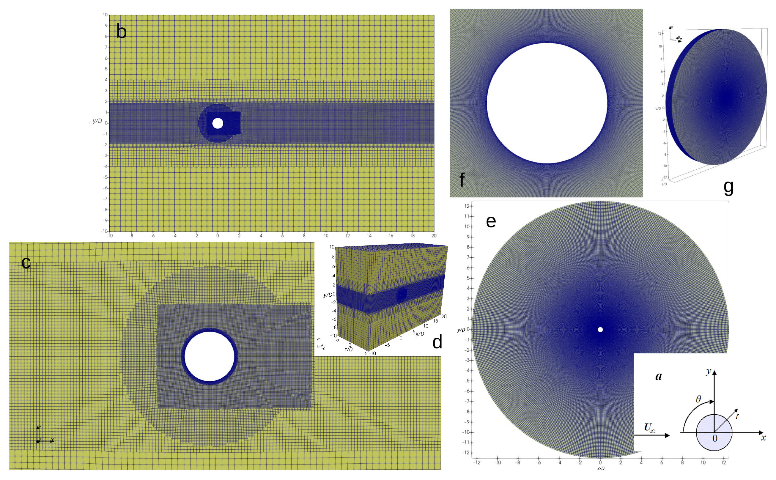
• Unstructured, hexahedral with different levels of adaptation (Figure 1b–d; used here and below the abbreviation HM). The computational domain is defined as a rectangular parallelepiped with dimensions $30D\times 20D\times 10D$ in the x, y, and z directions, respectively. As a starting point, the computational block was divided into $60\times 40\times 20$ nodes. Next, the grid was successively adapted in three iterations with a coefficient of $2\times 2\times 2$ in the regions from $y/D=-4$ to $y/D=4$, $y/D=-2.25$ to $y/D=2.25$, and $y/D=-1.9$ to $y/D=1.9$. The cylindrical region with a radius of $1.75$, located in the center of the Cartesian coordinates, was adapted at the next level with the same coefficient. The last iteration was applied to a rectangular region with dimensions $x/D=-1$ to $x/D=2$ and from $y/D=-1$ to $y/D=1$. Grid adaptation at all levels completely covered the computational region in the spanwise direction. Thus, the circumferential grid resolution of the cylinder is $N_{\theta }=184$, and along the span, $N_z=640$ ($L_z/D=0.0156$). For the adequate resolution of the boundary layer on the surface of the cylinder, a viscous sub-grid was added with a minimum dimensionless cell height, $y+=h_{1st}/D=4\times {10}^{-4}$, an expansion factor of $1.04$, and a total number of layers of 40, respectively. The total grid size is $2.43\times {10}^7$ cells.
• Curvilinear, orthogonal O-type (Figure 1e–g; used here and below the abbreviation OM) with a dimension of $444\times 444\times 64$ ($1.36\times {10}^7$ cells) in the x, y, and z directions, respectively. The length of the computational domain in the streamwise direction is $25\times D$, and in the spanwise direction, $L_z=\pi \times D$. The grid nodes are radially relaxed from the cylinder toward the outflow boundary with the dimensionless height of the first cell being $y^{+}=r/D=1.25\times {10}^{-4}$ and an expansion coefficient in the radial direction of $1.06$.

Two automatic grid partitioning techniques were used in the present simulations: METIS [33] and PT-Scotch [34], which are based on a graph partitioning approach and implemented in Ansys Fluent and OpenFOAM packages, respectively.

3. Brief Aspects of Mathematical Modeling and Numerical Simulations

The Favre-filtered balance equations for mass, momentum, and energy are

$${\displaystyle \frac{\partial \overline{\rho }}{\partial t}}+{\displaystyle \frac{\partial \overline{\rho }{\tilde{\mathbf{u}}}_j}{\partial x_j}}=0,$$

(1)

$${\displaystyle \frac{\partial \overline{\rho }{\tilde{\mathbf{u}}}_i}{\partial t}}+{\displaystyle \frac{\partial \overline{\rho }{\tilde{\mathbf{u}}}_i{\tilde{\mathbf{u}}}_j}{\partial x_j}}+{\displaystyle \frac{\partial \overline{p}}{\partial x_i}}-{\displaystyle \frac{\partial {\check{\sigma }}_{ij}}{\partial x_j}}=-{\displaystyle \frac{\partial {\tau }_{ij}}{\partial x_j}},$$

(2)

$${\displaystyle \frac{\partial \overline{\rho }\tilde{h}}{\partial t}}+{\displaystyle \frac{\partial \overline{\rho }\tilde{h}{\tilde{\mathbf{u}}}_j}{\partial x_j}}-{\displaystyle \frac{\partial \overline{p}}{\partial t}}-{\tilde{\mathbf{u}}}_j{\displaystyle \frac{\partial \overline{p}}{\partial x_j}}+{\displaystyle \frac{\partial \check{q_j}}{\partial x_j}}-{\check{\sigma }}_{ji}{\tilde{S}}_{ij}=-C_v{\displaystyle \frac{\partial Q_j}{\partial x_j}}.$$

(3)

The symbols $\rho$, p, and $\mathbf{u}$ represent density, pressure, and velocity, respectively. Enthalpy per unit mass, h, is given by $h=\epsilon +p/\rho$, with $\epsilon$ as internal energy per unit mass and T as temperature. The notations $\left(\overline{·}\right)$, $\left(\widetilde{·}\right)$, and $\left(\check{·}\right)$ indicate Reynolds-averaging, Favre-averaging, and filtering operations, respectively.

The conductive flux and viscous stresses are expressed as

$$\check{q_j}=-\kappa \left(\tilde{T}\right){\displaystyle \frac{\partial \tilde{T}}{\partial x_i}}$$

(4)

and

$${\check{\sigma }}_{ij}=2\mu \left(\tilde{T}\right)\left({\tilde{S}}_{ij}-{\displaystyle \frac{1}{3}}{\delta }_{ij}{\tilde{S}}_{kk}\right),$$

(5)

where the rate-of-strain tensor, ${\tilde{S}}_{ij}$, is

$${\tilde{S}}_{ij}={\displaystyle \frac{1}{2}}\left({\displaystyle \frac{\partial {\tilde{\mathbf{u}}}_i}{\partial x_j}}+{\displaystyle \frac{\partial {\tilde{\mathbf{u}}}_j}{\partial x_i}}\right).$$

(6)

Here, the viscosity, $\mu$, is calculated by Sutherland’s law and $\kappa$—conductivity.

For completeness, a filtered equation of state (EoS) is provided to close the system of governing equations using the ideal gas law:

$$\overline{p}=\overline{\rho }R\tilde{T}.$$

(7)

Assuming the sub-grid scales (SGS) incompressibility hypothesis [35,36], the SGS stress ${\tau }_{ij}$ and heat flux $Q_j$ can be expressed as follows:

$${\tau }_{ij}=\overline{\rho }\left(\widetilde{{\mathbf{u}}_i{\mathbf{u}}_j}-{\tilde{\mathbf{u}}}_i{\tilde{\mathbf{u}}}_j\right),$$

(8)

$$Q_j=\overline{\rho }\left(\widetilde{{\mathbf{u}}_{j}T}-{\tilde{\mathbf{u}}}_j\tilde{T}\right).$$

(9)

For closure, the k-equation eddy viscosity SGS model [37,38,39] and its dynamic version are used, based on the SGS kinetic energy $\tilde{k}={\displaystyle \frac{1}{2}}\left(\widetilde{\mathbf{u}·\mathbf{u}}-\tilde{\mathbf{u}}·\tilde{\mathbf{u}}\right)$. The SGS turbulence stresses are expressed as

$${\tau }_{ij}=-2{\mu }_B{\tilde{S}}_{ij}=-2c_k\overline{\rho }\sqrt{\tilde{k}}\Delta {\tilde{S}}_{ij},$$

(10)

with the SGS viscosity computed as

$${\mu }_B=c_k\overline{\rho }\sqrt{\tilde{k}}\Delta ,$$

(11)

where $\Delta$ is the filter length. The transport equation used to estimate $\tilde{k}$ is

$${\displaystyle \frac{\partial }{\partial t}}\left(\overline{\rho }\tilde{k}\right)+{\displaystyle \frac{\partial }{\partial x_j}}\left(\overline{\rho }{\tilde{\mathbf{u}}}_j\tilde{k}\right)=F_p+F_d-F_{ϵ},$$

(12)

where production $F_p$, diffusion $F_d$, and dissipation $F_{ϵ}$ are expressed as

$$F_p=-\mathbf{B}·\tilde{\mathbf{D}},$$

(13)

$$F_d={\displaystyle \frac{\partial }{\partial x_j}}\left(({\mu }_B+\mu ){\displaystyle \frac{\partial \tilde{k}}{\partial x_j}}\right),$$

(14)

$$F_{ϵ}=c_{ϵ}\overline{\rho }{\tilde{k}}^{3/2}/\Delta ,$$

(15)

$$\mathbf{B}={\displaystyle \frac{2}{3}}\overline{\rho }\tilde{k}\mathbf{I}-2{\mu }_B{\tilde{\mathbf{D}}}_D,$$

(16)

$${\tilde{\mathbf{D}}}_D=\left[\tilde{\mathbf{D}}-{\displaystyle \frac{1}{3}}\left(\mathrm{tr}\tilde{\mathbf{D}}\right)\mathbf{I}\right],$$

(17)

$$\tilde{\mathbf{D}}={\displaystyle \frac{1}{2}}\left(\mathrm{grad}\tilde{\mathbf{u}}+\mathrm{grad}{\tilde{\mathbf{u}}}^{\mathrm{T}}\right).$$

(18)

Here, $\mathbf{I}$ is the unit tensor, $\mathbf{B}$ is the density-weighted stress tensor, ${\tilde{\mathbf{D}}}_D$ is the deviatoric part of the rate of strain tensor, and the model coefficients are $c_k=0.07$ and $c_{ϵ}=1.048$ [40]. The dynamic model for the k-equation can be derived using the Germano identity with another filter kernel of width $\overline{\Delta }=2\Delta$ (the theoretical background can be found in [35]).

Large-eddy simulation is performed using the CFD platforms Ansys Fluent 2021R1 [41] and OpenFOAM v2212 [42] (hereinafter, the abbreviations AF and OF are used, respectively). To close the filtered, Favre-averaged Navier–Stokes equations, the differential sub-grid scale model for the turbulence kinetic energy (k-model) and its dynamic modification are used. Both numerical platforms are based on the finite volume method (FVM) implemented as a pressure-based solver [43] using a limited central differencing scheme of the second-order (bounded CDS-2) for the velocity, a second-order upwind scheme (SOU) for the remaining nonlinear convective terms, and an implicit Euler method (bounded BDF-2) for time integration [35]. The time integration step is chosen to ensure that the local Courant number is less than one ($\mathrm{CFL}<1$). The system of linear algebraic equations is solved using the algebraic multigrid method (AMG) accompanied by the additive correction strategy [44] and the classical iterative Gauss–Seidel procedure in AF and the symmetric iterative Gauss–Seidel method for all dependent variables except pressure, which is calculated using the geometric multigrid method (GAMG) [45] in OF.

For the spectral analysis of time series, the classical methods of the fast Fourier transform (FFT), Welch periodograms [46], and continuous wavelet transform (CWT) are used, detailed descriptions of which can be found in [1]. The Lyapunov metric, described in detail in our previous work [3], is used to study the phase properties of dynamic systems.

The formulation of boundary and initial conditions is similar to that presented earlier [1] with the exception of setting the velocity field at the inlet boundary and corresponds to the free-stream values of the Reynolds and Mach numbers $\mathrm{R}\mathrm{e}$ = 130,000 and $\mathrm{M}=0.05$. The inlet boundary conditions (on the left side of the computational domain) were treated as laminar. At the outlet, wave-transmissive or non-reflecting conditions were applied. Isothermal no-slip conditions were enforced on the cylinder’s surface. Periodic flow was assumed in the spanwise direction of the cylinder. The initial conditions corresponded to the sudden stopping of a cylinder in a fluid flow, meaning the inflow conditions were initially extended throughout the entire computational region. The ideal gas law is used to account for compressibility. Molecular viscosity and thermal conductivity are assumed to be constant. The Prandtl number was taken to be $0.75$, and the ratio of specific heat capacities was $1.4$.

The characteristic convective time is defined as the ratio of the streamwise length of the computational domain to the free-stream velocity, ${\tau }_{conv}=L_x/U_{\infty }$. The solution is considered statistically converged after ${\tau }_{conv}>4$. To obtain statistically independent data, time averaging is performed over an interval equal to $N_{vs}=25$ (here, $N_{vs}$ is the vortex shedding cycle or the period of oscillatory motion). The averaging operator is denoted as 〈〉.

4. Results

The runs matrix is given in

Table 1. Runs matrix: numerical platform, floating-point arithmetic, computational grid, and sub-grid scale model.

Run	CFD Code	Precision	Mesh	TM
OF-TKE	OF	DP	HM	TKE
OF-dTKE	OF	DP	HM	dTKE
OFm-dTKE	OF	SPDP	OM	dTKE
AF32-dTKE	AF	SP	OM	dTKE
AF64-dTKE	AF	DP	OM	dTKE
T-AF32-dTKE	AF	SP	HMT	dTKE
T-AF64-dTKE	AF	DP	HMT	dTKE

. It should be noted that LES using OF were performed on an unstructured hexahedral grid, while the O-type grid was used to study the effects of single- and double-precision arithmetic using AF. The following sub-grid scale models were tested: the differential model for the kinetic energy (or the k-model, with coefficients $C_k=0.07$ and $C_{ϵ}=1.042$, hereinafter TKE) and its dynamic modification (hereinafter dTKE). The results are compared with the experimental data of Achenbach [17], Cantwell and Coles [14], Schewe [22], Norberg [27], and Lim and Li [29] and LES data presented by Breuer [9], Cao and Tamura [10], Lloyd and James [11], Yeon et al. [12], and Plata et al. [13]. A critical remark should be made here: in physical experiments of external aerodynamics, an important factor is the turbulence intensity and the uniformity of the incoming flow, which in turn is determined by the quality of a wind tunnel. Sometimes, there is a possibility that the laminar–turbulent transition will occur directly in the boundary layer before its separation from the bluff body surface. In this case, a number of integral parameters, such as the separation angle, pulsations of the lift coefficient, and the length of the recirculation zone, can be significantly overestimated/underestimated. In addition, a flow bifurcation is possible, as in the case of the flow over a circular cylinder at $\mathrm{R}\mathrm{e}=3900$ [3].

4.1. Instantaneous Flow Field

The dynamics of the lift and drag coefficients over time are shown in Figure 2. Figure 3 illustrates the formation of a vortex street and coherent energy structures using the Q-criterion, $Q=S^2-{\Omega }^2={10}^4$ (where S is the strain rate tensor and $\Omega$ represents the vorticity). Figure 4 shows the probability density function of the normalized lift coefficient $C_l$. Two different forms of probability distribution obtained for the AF32-dTKE, AF64-TKE and OF-TKE, OF-dTKE runs, respectively, are clearly visible. OF-TKE (and it seems OF-dTKE as well) has a distribution close to bi-modal, having two widely spaced and symmetrical peaks. For AF32-dTKE and AF64-dTKE, the histograms reproduce the shape of the Gaussian curve (or normal distribution) quite well. In practice, for the sub-critical flow over a cylinder, the normal distribution of $C_l$ obtained by Schewe [22], as well as in the numerical results obtained by Cao and Tamura [10], is confirmed. The physical interpretation of this phenomenon is that random modulations of amplitude and frequency during the formation and shedding of vortices and their subsequent convection downstream from the wake contribute to the formation of a distribution close to normal [10]. The difference in probability density distributions between AF32-dTKE, AF64-TKE and OF-TKE, OF-dTKE may explain the observed variations in aerodynamic coefficients in Figure 2. It should also be considered that the time integration interval used in this study may not be large enough to obtain a fully statistically converged flow field.

4.2. Integral Parameters

Table 2. Review of experimental and LES studies for the turbulent flow over a circular cylinder at $\mathrm{Re}$ = 130,000: parameters and integral characteristics.

Source	Method	$\langle {\mathit{C}}_{\mathit{d}}\rangle$	$\langle {\mathit{C}}_{\mathit{l}}^{\prime }\rangle$	$\mathbf{St}$	$-\langle {\mathit{C}}_{\mathit{p},\mathit{b}}\rangle$	$\langle {\mathit{L}}_{\mathit{r}}/\mathit{D}\rangle$	${\mathit{\theta }}_{\mathit{s}}$
Achenbach [17]	HWA	1.19			1.25		78
Cantwell & Coles [14]	HWA	1.24	0.52	0.179	1.21	0.4–0.5	77
Schewe [22]	HWA	1.17	0.25	0.20
Norberg [27]			0.49	0.185
Lim & Lee [29]	HWA	1.2		0.185	1.15
Breuer (DC) [9]	LES	1.28		0.22	1.51	0.46	94
Breuer (D3) [9]	LES	1.37		0.21	1.6	0.42	91
Cao & Tamura [10]	LES	1.16	0.3	0.2
Lloyd & James (4C) [11]	LES	1.00	0.63	0.177	1.01
Lloyd & James (4F) [11]	LES	0.89	0.5	0.203	0.86
Yeon et al. [12]	LES	1.37	0.62	0.2	1.64	0.63	81
Plata et al. [13]	LES	1.43		0.19	1.59	0.5
Present work
$\mathrm{OF}-\mathrm{TKE}$	LES	1.33	0.41	0.19	1.36	0.55	83°
$\mathrm{OF}-\mathrm{dTKE}$	LES	1.34	0.53	0.19	1.37	0.58	83°
$\mathrm{OFm}-\mathrm{dTKE}$	LES	0.98	0.55	0.18	1.03	0.62	89°
$\mathrm{AF}32-\mathrm{dTKE}$	LES	0.94	0.28	0.21	1.01	0.68	85°
$\mathrm{AF}64-\mathrm{dTKE}$	LES	0.94	0.27	0.21	1.01	0.68	85°
$\mathrm{T}-\mathrm{AF}32-\mathrm{dTKE}$	LES	1.01	0.30	0.22	0.95	0.67	89°
$\mathrm{T}-\mathrm{AF}64-\mathrm{dTKE}$	LES	1.01	0.31	0.22	0.95	0.67	89°

presents the main integral flow parameters, such as the lift ($C_l$), drag ($C_d$), and pressure base suction ($C_{pb}$) coefficients, the Strouhal number (${St}_p$), the separation zone length ($L_r$), and the primary boundary layer separation angle ${\theta }_s$.

The distribution of the pressure coefficient $\langle C_p\rangle =2(\langle p\rangle -p_{\infty })/\left({\rho }_{\infty }{U}_{\infty }^2\right)$ (here, $p_{\infty }$ is the free-stream pressure) over a circular cylinder is shown in Figure 5a. The numerical results obtained by OF-TKE, OF-dTKE are in satisfactory agreement with the experiments of Cantwell and Cowles [14] and Lim and Li [29], as well as with the numerical data of Cao and Tamura [10] and Yeon et al. [12], while the $\langle C_p\rangle$ distributions by AF32-dTKE and AF64-dTKE better approximate the experimental data of Achenbach [17].

In Figure 5b, the friction coefficient along the cylinder surface $\langle C_{\tau }\rangle =2(\langle \tau \rangle -p_{\infty })/\left({\rho }_{\infty }{U}_{\infty }^2\right)$ (here, $\tau$ is the friction) obtained in the present LES is compared with the experiment by Achenbach [17]. The OF-TKE, OF-dTKE runs are in satisfactory agreement with the numerical data of Yeon et al. [12] and qualitatively reproduce distributions by Achenbach [17]. It should be noted that the experimental measurements of Achenbach [17] for $\mathrm{Re}$ = 100,000 are used. The AF32-dTKE and AF64-dTKE runs show qualitative agreement with the data of Achenbach [17] starting from the stagnation point (${\theta }_s=0^{\circ }$) to the separation point $\theta \approx {80}^{\circ }$. The separation angle ${\theta }_s$ is determined from the condition of zero shear stress on the cylinder surface. From the experiments of Achenbach [17] and Cantwell and Cowles [14], the boundary layer separation occurs at ${\theta }_s$ = 77–${78}^{\circ }$. The computed values of ${\theta }_s$ are slightly overestimated as ${\theta }_s$ = 83–${85}^{\circ }$ but are consistent with the data of Yeon et al. [12] (${\theta }_s={81}^{\circ }$). In the results obtained by Breuer [9], the separation point is shifted even further downstream ${\theta }_s$ = 91–${94}^{\circ }$. The nature of the curves $\langle C_{\tau }\rangle$ obtained in the simulations on the back side of the cylinder indicates the presence of secondary vortex structures, however, due to the lack of experimental data, their quantitative assessment is not given here.

The mean base suction coefficient $\langle C_{p,b}\rangle$ is defined as the pressure coefficient on the cylinder surface at the point where $\theta ={180}^{\circ }$. Its values computed by OF-TKE, OF-dTKE, AF32-dTKE, and AF64-dTKE were $\langle -C_{p,b}\rangle =1.36$ and $\langle -C_{p,b}\rangle =1.01$, respectively. At the same time, the experimental results yield values in the range of $\langle -C_{p,b}\rangle$ = 1.15–1.25 [14,17,29]. A wide range of values of $\langle C_{p,b}\rangle$ is also observed in the available LES works: from $\langle -C_{p,b}\rangle$ = 0.86–1.01 [11] to $\langle -C_{p,b}\rangle$ = 1.51–1.64 [9,12,13].

The base suction pressure coefficient is related to the drag ($C_d$) and lift ($C_l$) coefficients, which are calculated by integrating the pressure over the cylinder surface: $C_d=2F_x/\left({\rho }_{\infty }{U}_{\infty }^{2}A\right)$ and $C_l=2F_y/\left({\rho }_{\infty }{U}_{\infty }^{2}A\right)$. Here, $F_x$ and $F_y$ are the forces acting on the cylinder in the streamwise and vertical directions, respectively. $A=L_z\times D$ is the surface area of the cylinder projected along the span. The mean drag coefficient was $\langle C_d\rangle =1.34$ for OF-TKE, OF-dTKE and $\langle C_d\rangle =0.94$ for AF32-dTKE and AF64-dTKE, respectively. The experimental value of the drag coefficient converges to $\langle C_d\rangle =1.2$ [14,17,22,29], except in the data provided in the NACA-TM-3038 report [16], where $\langle C_d\rangle \approx$ 0.95–1.05 is presented. The numerical values obtained from different LES studies show a large scatter $\langle C_d\rangle$ = 0.89–1.43 [9,10,11,12,13]. It is interesting to note that the mean value predicted by LES, including the present results, converges to $\langle C_d\rangle =1.19\pm 0.2\%$ with a dispersion of about $20\%$. The lift coefficient pulsations obtained in the present work ($\langle C_l^{\prime }\rangle$ = 0.27–0.41) are consistent with the available experimental ($\langle C_l^{\prime }\rangle$ = 0.25–0.52 [14,22,27]) and numerical ($\langle C_l^{\prime }\rangle$ = 0.3–0.63 [10,11,12]) data.

An important parameter is the length of the recirculation zone $L_r$, defined as the distance between the base of the cylinder and the sign change of the centerline mean streamwise velocity. It is well-known that the measurement of $L_r$ in experiments often strongly depends on the early laminar–turbulent transition in separated shear layers, usually caused by the incoming turbulence intensity, when the early transition corresponds to a shorter length of the separated zone [3,47]. From the LES point of view, the important parameters are the statistical convergence [48], the free-stream turbulence intensity [3], the spanwise length of the computational domain [10], and, in general, the numerical dissipation of the computational methodology (grids, convective schemes, algorithms, etc.) [9,11,12,13]. The experimental values of the recirculation zone length are limited by the data of Cantwell and Cowles [14], $L_r$ = 0.4–0.5. These values correlate quite satisfactorily with the numerical data of [9,12,13], $L_r$ = 0.42–0.63, and the present results obtained by OF-TKE and OF-dTKE, $L_r$ = 0.55–0.58. At the same time, AF32-dTKE and AF64-dTKE show $L_r=0.68$ when the length of the separation zone significantly exceeds the experimental measurements [14].

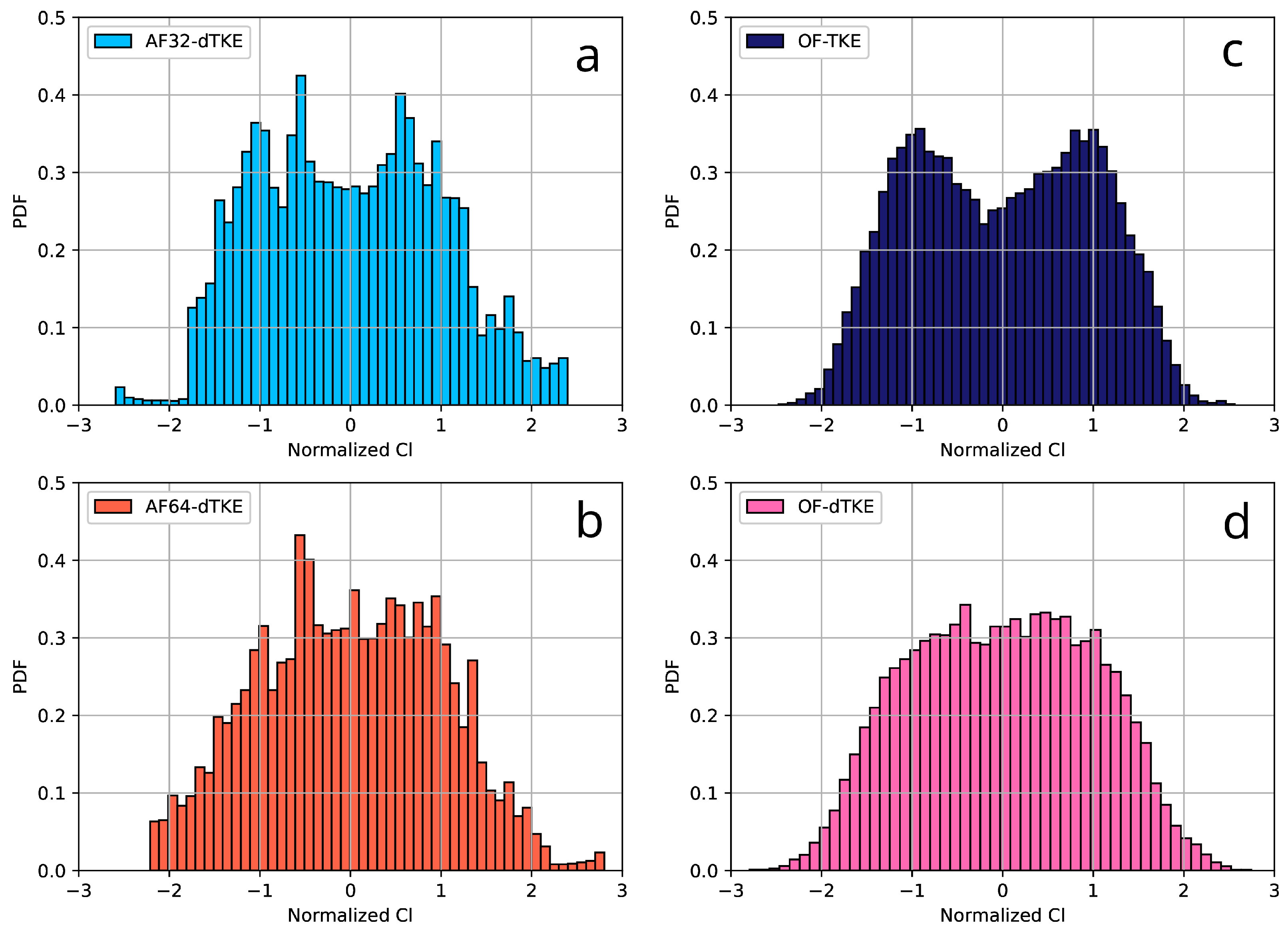
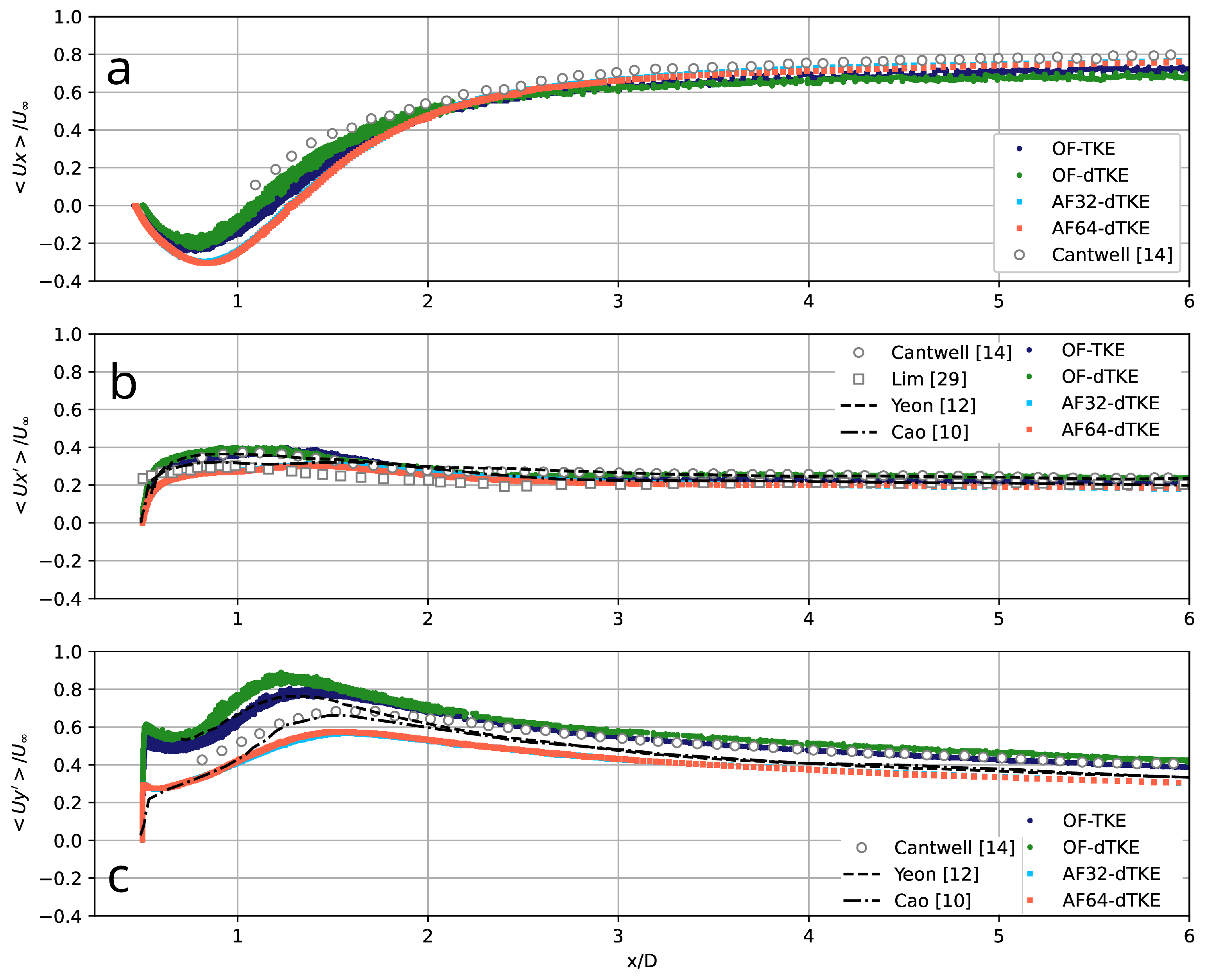
4.3. First- and Second-Order Statistics

The distribution of the mean streamwise velocity $〈U_x〉$ along the central axis is shown in Figure 6a. It is clearly seen that the present LES is in satisfactory agreement with the experiment by Cantwell and Coles [14] in the far wake ($x/D>2$), while in the vicinity of the cylinder, the results generally overestimate the length of the recirculation zone. It is interesting to note that the flow intensity (minimum values of the streamwise velocity) in the core of the separation zone obtained by AF32-dTKE and AF64-dTKE differs by approximately $1.5$ times from the values obtained by OF-TKE and OF-dTKE.

The pulsations of the streamwise velocity $〈U_x^{\prime }〉$ along the central axis (Figure 6b) obtained by OF-TKE and OF-dTKE are in satisfactory agreement with measurements made by Cantwell and Coles [14] and with the LES data of Cao and Tamura [10] and Yeon et al. [12]. The results obtained by AF32-dTKE and AF64-dTKE are closer to the experiment by Lim and Lee [29].

The predicted pulsations of the vertical velocity $〈U_y^{\prime }〉$ along the central axis and experiment data of Cantwell and Coles [14] are compared in Figure 6c. The results obtained by AF32-dTKE and AF64-dTKE match the numerical data of Cao and Tamura [10] and are underestimated by about $15\%$ compared with the experiment of Cantwell and Coles [14]. The results obtained by OF-TKE and OF-dTKE diverge by about $30\%$ from the physical measurements in the near wake ($x/D<2$), after which they begin to converge smoothly. The same trend is observed in the LES results obtained by Yeon et al. [12].

In Figure 7, the predicted and experimental profiles of the mean streamwise and vertical velocities in the radial cross-section of the computational domain are compared at $x/D=1$, $1.5$, and 2. The deficit observed in the present LES in all three cross-sections for the streamwise velocity with respect to the experimental data is explained by the general overestimated value of the separation zone length. For the vertical velocity, satisfactory agreement was obtained between the present LES and experiment by Cantwell and Coles [14], with the exception of $x/D=1$, where a small disagreement was also observed for AF32-dTKE and AF64-dTKE. Figure 7 shows the radial profiles of the root-mean-square values of the normal Reynolds stresses, $\langle U_x^{\prime }{U}_y^{\prime }\rangle$, where, in general, qualitative agreement between the present and experimental data is observed. The discrepancies for the peak values are approximately $20\%$.

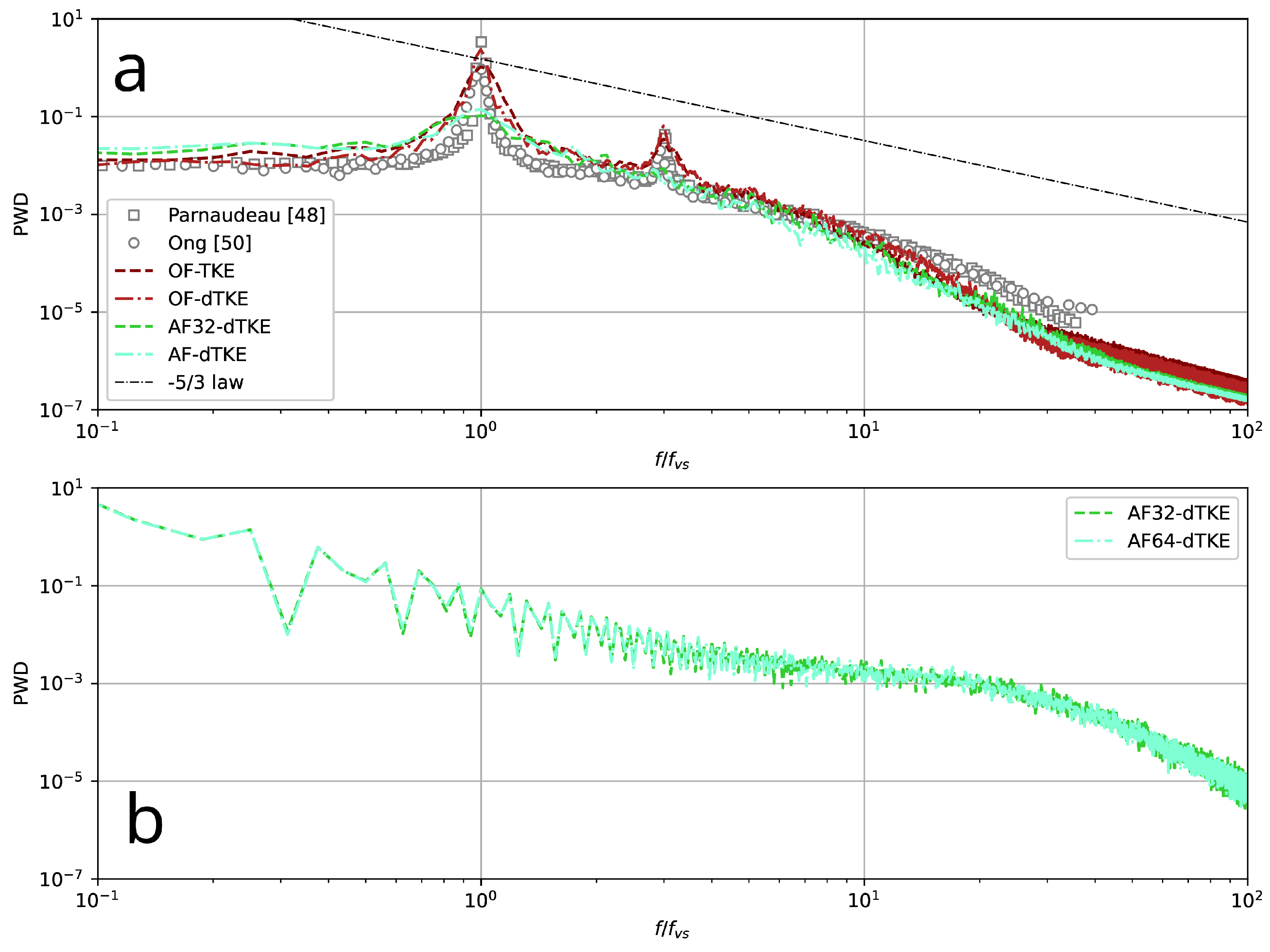
4.4. One-Dimensional Energy Spectra

The flow over a circular cylinder at $\mathrm{Re}=$ = 130,000 belongs to the sub-critical regime when the boundary layers remain laminar ($1000<\mathrm{Re}$ < 200,000). In this range of Reynolds numbers, both absolute and convective instabilities are present: asymmetric vortex shedding (Benard/von Kármán) and Kelvin–Helmholtz (KH) in the shear layer [49]. The vortex instability is periodic and has a characteristic frequency $f_{vs}=\mathrm{St}{U}_{\infty }/D$, where $\mathrm{St}$ is the Strouhal number. Using FFT for the vertical velocity in the near wake of the cylinder ($x/D=1.5,y/D=0$), the computed Strouhal numbers were $\mathrm{St}=0.19$ for AF32-dTKE and AF64-dTKE, and $\mathrm{St}=0.21$ for OF-TKE and OF-dTKE, respectively. It should be noted that if FFT is applied for the lift coefficient, the Strouhal numbers are slightly different: $\mathrm{St}=0.19$ and $\mathrm{St}=0.18$ for AF32-dTKE, AF64-dTKE and OF-TKE, OF-dTKE, respectively. The experimental value of the Strouhal number for $\mathrm{Re}$ = 130,000 varies within $\mathrm{St}$ = 0.18–0.20 [14,22,27,29]. The LES data from Table 2 also show a small dispersion, $\mathrm{St}$ = 0.177–0.22.

In Figure 8a, the one-dimensional energy spectra, normalized by the characteristic Strouhal frequency ($f_{vs}$), are compared with the experimental measurements of Ong and Wallace [50], Parnaudeau et al. [48], and the $-5/3$ power law. The Welch’s periodogram technique [46] is used to smooth the spectral curves. Also, to increase the statistical significance [47], the spectra are averaged in the spanwise direction. It is well known that the effect of the excessive dissipation of the numerical method usually leads to the rapid attenuation of the spectrum and unsatisfactory reproduction of the inertial interval [1,47,51]. In the present work, the inertial interval is clearly reproduced over a wide range of wave numbers, which agrees well with the experiments by Ong and Wallace [50] and Parnaudeau et al. [48]. The presence of small-scale, coherent energy structures that remain active far from the cylinder is shown in Figure 3. All predicted curves in Figure 8a collapse satisfactorily up to $f/f_{vs}\approx 1$, after which they begin to decay slowly.

The dynamics of boundary layer separation are similar to the mixing layer when the length of the recirculation zone is large enough. The Kelvin–Helmholtz (KH) mechanism underlying the shear layer instability has a characteristic frequency ($f_{kh}$) for $\mathrm{Re}>1200$ at which the mixing layer collapses into highly concentrated vortices [52]. At present, a sufficiently large amount of experimental data has accumulated to analyze the dependence of the characteristic frequency of the mixing layer on the Reynolds number for various simple geometric figures. Some data are presented in Figure 9, and the reader can find a further analysis of them in [6,7].

In the LES framework of the flow over a circular cylinder at $\mathrm{Re}=3900$ [1] and $\mathrm{Re}$ = 20,000 [4], the values $f_{kh}/f_{vs}$ = 7–8 and $f_{kh}/f_{vs}=16.2$ were computed, respectively. These results are in good agreement with the available experimental and numerical results [53]. In the work of Cao and Tamura [10] for $\mathrm{Re}$ = 130,000, the numerical values of the characteristic peak frequencies $f_{kh}/f_{vs}$ = 15–17 are presented. The present LES for $\mathrm{Re}$ = 130,000 (AF32-dTKE and AF64-dTKE) are in the range of $f_{kh}/f_{vs}\approx 28.9$. Based on these numbers, it is possible to show a quadratic dependence of the characteristic instability frequency on the Reynolds number of the form $\sqrt{\mathrm{Re}}$, taking into account the thickness and separation velocity of the laminar boundary layer, which is in good agreement with Bloor [54], who established the exponent, $n=0.67$: $f_{kh}/f_{vs}=A\times {Re}^{0.67}$. The present results are well approximated by the adjusted value $n=0.65$ (Figure 9).

Figure 9. Dependence of the normalized characteristic frequency of the separated shear layers on the Reynolds number: results of numerical and physical modeling. Here CC, SC, TC and HC—abbreviations for the circular, square, triangular and semi-circular cylinders, respectively. Experimental and numerical data collected from [1,4,6,7,54,55,56,57,58,59,60,61,62,63,64,65].

Figure 9. Dependence of the normalized characteristic frequency of the separated shear layers on the Reynolds number: results of numerical and physical modeling. Here CC, SC, TC and HC—abbreviations for the circular, square, triangular and semi-circular cylinders, respectively. Experimental and numerical data collected from [1,4,6,7,54,55,56,57,58,59,60,61,62,63,64,65].

Figure 8b shows the curves of the energy spectra, where a relatively broadband frequency range of $f_{kh}/f_{vs}$ is visible. To quantitatively estimate the average frequency of the KH instability, the one-dimensional wavelet transform is used. Figure 10 presents the CWT results for the vertical velocity measured in the shear layer near the vicinity of the circular cylinder for the different Reynolds numbers. It is clearly seen that both the BK and KH instabilities occur only periodically and have an intermittent character. The KH peaks do not always appear at the same frequency but are localized in a certain frequency range and also depend on time. A tendency for the energy density to increase with increasing Reynolds number is clearly visible.

4.5. Lyapunov Metric

In this section, an attempt is made to quantitatively and qualitatively estimate the difference between the two dynamic systems, AF32 and AF64, using the Lyapunov metric. The modified procedure, proposed by Nastak et al. [66] and later adapted by Lysenko [3], is used for the LES of the flow over a circular cylinder.

To solve the problem, the same numerical methodology and computational grid (similar to AF32-dTKE and AF64-dTKE) are utilized. Two scenarios are investigated. In the first case, single-precision arithmetic is used, while in the second, double-precision arithmetic is employed. The simulations start at the same time $t_0$. Both solutions are initialized with statistically converged data after reaching the convective time ${\tau }_{conv}=4$. Figure 11 compares the difference in phase trajectories obtained for two solutions, AF32 and AF64. To calculate the divergence, the $L_2$-norm is used, and it is assumed that the process is ergodic (the Lyapunov exponent does not depend on the initial conditions when the level of initial perturbations is sufficiently small: $ϵ\ll 1$ [67]). In this case, the initial perturbations are the loss of accuracy due to round-off errors when going from DP to SP, i.e., for the C and C++ programming languages (in which both numerical platforms are implemented), $ϵ\approx \parallel 2^{-52}-2^{-23}\parallel$. The presented time evolution of the separation is similar to the work of Nastak et al. [66] and contains two domains: the linear region and the saturation region. It can be noted that the divergence increases with time when the velocity fields first diverge from small structures to larger homogeneous isotropic structures over time [3,66]. Also, in Figure 11c, there is a well-defined region of the so-called initial pulse (the initial response region) [66] which is absent in the phase trajectories for the streamwise and vertical velocities.

The Lyapunov exponent is estimated from the slope of the separation curve in the logarithmic region and is shown as dashed lines in Figure 11. The slope of the Lyapunov exponent is related to the predictability time [66], which corresponds to $t_p$∼$1.5{\tau }_{conv}$. In practice, the predictability time shows how quickly a dynamic system will transit from one state to another [3]. According to [66], the predictability time and the Lyapunov exponent can be used as quantitative information about the time horizon over which the phase transition can be modeled. The Lyapunov metric can also be used to study the stability of dynamic systems. Thus, an important conclusion and a direct consequence of Figure 11 is that the dynamic system AF32 is stable by Lyapunov [68]. From Figure 11, it is clearly seen that after reaching the predictability time, saturation occurs, since the divergence of phase trajectories reaches an asymptotic: a statistically stationary state of both systems is reached.

Under some considerations, it can be assumed that the concepts of turbulence and chaos are closely related [3,69,70]. Thus, the concept of an attractor for nonlinear dynamic systems from the chaos theory can be applied to the analysis of turbulent flows described by the Navier–Stokes equations. To reconstruct attractors, i.e., states of the phase space or the evolution of the system from the initial conditions, one can use a three-dimensional time signal of the computed norm of the dimension p, $\parallel L_p\parallel \equiv {\left(1/V{\int }_V{(·)}^{p}dV\right)}^{1/p}$ (where V is the volume of the computational domain) using the Takens embedding method [71] in the same spirit as Alberti et al. [70] and Lysenko [3]. In practice, the second-order norm can be used to examine the behavior of the attractor in the phase space: $\mathrm{\Theta }\left(t\right)=\left[{\displaystyle \frac{d\parallel U_x\parallel }{dt}},{\displaystyle \frac{d\parallel U_y\parallel }{dt}},{\displaystyle \frac{d\parallel U_z\parallel }{dt}}\right]$ (here, the symbol t denotes time). Figure 12 shows the evolution of the AF32 and AF64 attractors in the three-dimensional space as well as the results obtained by Lysenko [3] for $\mathrm{Re}=3900$. It is evident that the results for $\mathrm{Re}=3900$ and $\mathrm{Re}$ = 130,000 are quite consistent, and the dimension of the attractors for $\mathrm{Re}$ = 130,000 significantly exceed the case for $\mathrm{Re}=3900$. Similarly to Lysenko [3], all systems are limited to simple geometric figures, ellipsoids.

5. Discussion

Large-eddy simulations of the flow over a circular cylinder at $\mathrm{Re}$ = 130,000 were carried out in order to assess the following goals and objectives:

• Further validation and verification of LES for the external aerodynamics and turbulent separated flows. Previously, the turbulent flows over circular ($\mathrm{Re}=3900$ [1,2,3] and $\mathrm{Re}$ = 20,000 [4]), semi-circular ($\mathrm{Re}$ = 50,000 [7]), and triangular ($\mathrm{Re}$ = 45,000 [5,6]) cylinders were studied in detail. The differential sub-grid scale k-model (with constants $C_k=0.07$ and $C_{ϵ}=1.048$) and its dynamic modification were tested. In the present work, the Reynolds number was increased by almost an order of magnitude to $\mathrm{Re}$ = 130,000. Also, in addition to OF, numerical simulations was extended to use the commercial CFD code AF.
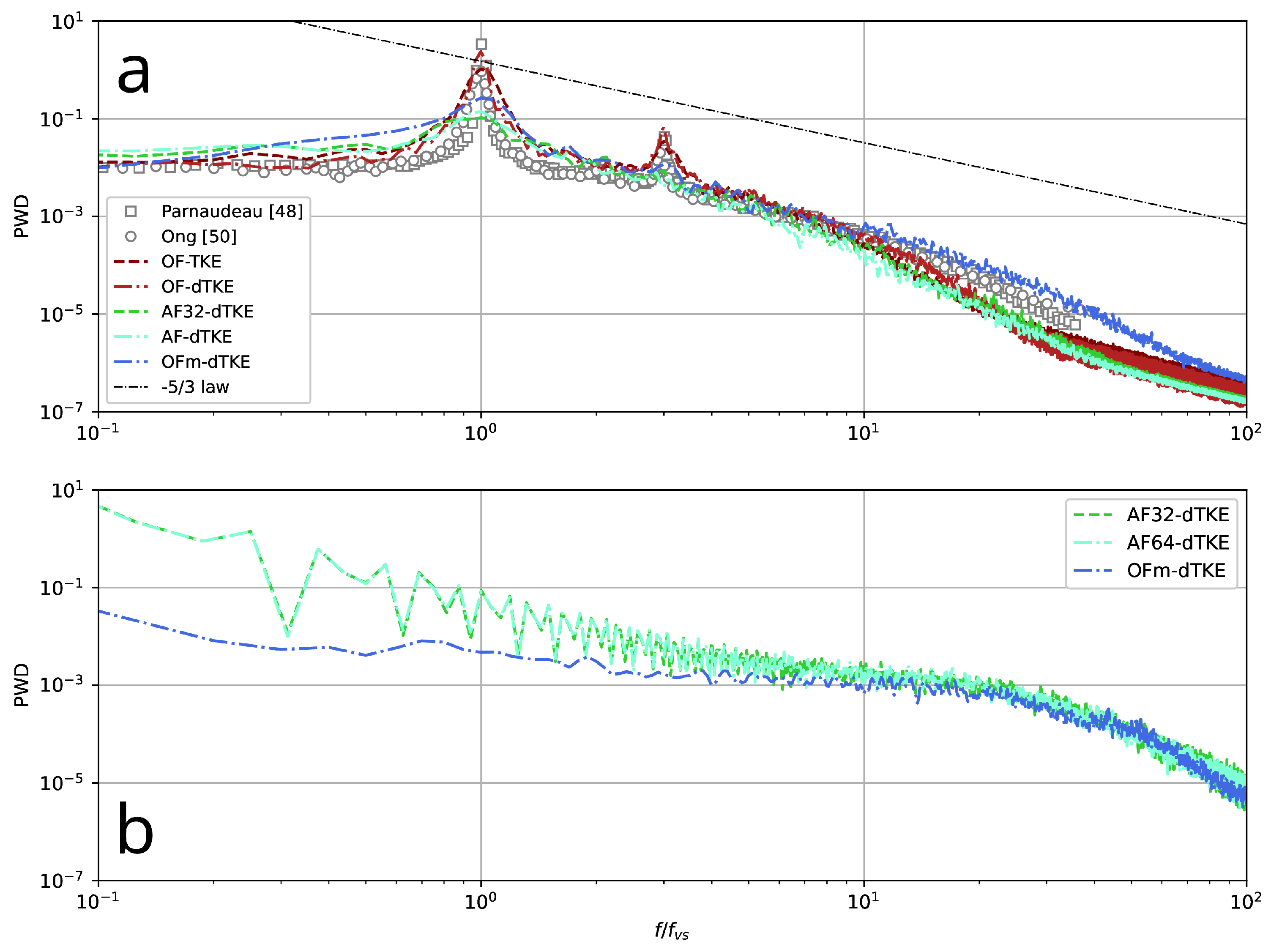
• Investigation of LES and related numerical methods using single-precision arithmetic, which is also due to several factors. The most important is the possibility of the more efficient use of computational resources: on the one hand, numerical methods using SP arithmetic use less RAM and, as a rule, provide a small performance gain (≈10–20%) when using classical CPUs. On the other hand, they allow for achieving significant acceleration on graphics accelerators, which are usually optimized for single-precision calculations, as well as on hybrid CPU–GPU systems.
  As mentioned above, OF provides the ability to perform simulations using mixed-precision arithmetic, SPDP. To test it, another special run (OFm-dTKE) was performed using the O-type grid. In this case, the problem was set up as closely as possible to match the AF32-dTKE and AF64-dTKE runs. On the one hand, the predicted integral flow characteristics (Table 2) converge with a small variation to the data obtained by AF32-dTKE and AF64-dTKE, which indicates the reasonable consistency of the two numerical platforms. On the other hand, the numerical method implemented in OF, even for the SPDP case, has a smaller numerical diffusion, which is clearly seen in Figure 13, where the one-dimensional energy spectra are compared. Numerical dissipation is clearly visible for the AF32-dTKE and AF64-dTKE runs. It should be noted that it was not possible to obtain a final physical solution using OF with single-precision arithmetic (similarly to Brogi et al. [32]). Most likely, this is due to the fact that the linear algebra algorithms implemented in OF are more sensitive to high-frequency perturbations due to round-off errors. It is also worth emphasizing that in the present work, the dynamic differential sub-grid scale model for the kinetic energy was used, which is strictly dissipative under the condition that the turbulent viscosity is positive [35], i.e., it makes a certain contribution to the suppression of high-frequency oscillations, which, together with the algebraic multigrid method implemented in AF, allows for the effective simulation of the turbulent flows with single precision.
• Qualitative and quantitative testing of LES implemented in two numerical platforms, AF and OF, using coarse and medium-sized computational grids (10–25 M cells) for the Reynolds number of practical interest ($\mathrm{Re}$ = 130,000). Curved, orthogonal O-type (OM) and unstructured, hexahedral (HM) meshes, with several levels of computational adaptation, are used.

In general, the present LES reproduced the physics of the flow over a cylinder, consisting of several important mechanisms. First of all are the occurrence of the Kelvin–Heimholtz instability in the separated shear layers, further growth and development of disturbances on the discontinuity interface and the subsequent laminar–turbulent transition, and the development of vortex cores and their convection downstream (asymmetric vortex formation or Benard/von Kármán instability). The vortex dynamics in the wake, characterized by the Strouhal number, are in satisfactory agreement with the available data. Since it was not possible to find any values for the Kelvin–Heimholtz instability for the Reynolds number $\mathrm{Re}$ = 130,000, the values obtained in this work are difficult to quantify. Qualitatively, they are well approximated by the value $n=0.65$ for the power law dependence proposed by Bloor [54]. The root-mean-square values of lift pulsations are in good agreement with the available LES and experimental data. The predicted drag coefficients are within the range of values presented in the literature. Another important parameter is the length of the separation zone. The present work shows quite large discrepancies between simulations and measurements. Other authors also show significant scatter. It should be noted that for a given Reynolds number, there is only one experiment [14]. A wide variety of factors influence the quality of LES (computational grids and their dimensions, boundary conditions, convective schemes, sub-grid scale models, numerical methods, etc.), and it is difficult to single out several fundamental ones that influence the prediction of $C_d$ and $L_r$.

Despite the fact that, in general, satisfactory agreement has been achieved for a number of integral and local parameters, the found deviations for $C_d$ and $L_r$ indicate that this test case for $\mathrm{Re}$ = 130,000 is still a ’challenge’ problem for the large-eddy simulations. This is primarily due to limited computational resources, which are usually bounded by the following factors:

• The overall performance of the computing system, which is usually limited by the execution time (the time per step per grid node, which is now effectively fixed, since the processor clock rate does not increase) and the number of effective MPI nodes, which depends on the problem size and the network communication rate. Parallel efficiency is also usually limited to about $70\%$ of the theoretical one in the case when pressure-based algorithms are used and the stability condition ($\mathrm{CFL}<1$) is imposed by the computational grid and the boundary layer resolution ($y^{+}<1$);
• The final period of time integration (the total number of time integration steps), consisting of the interval required to obtain a statistically converged flow field (reaching the self-oscillatory regime, on the order of several ${\tau }_{conv}$) and the time segment required to get time-averaged data (usually several tens of $N_{vs}$).

It is important to note that in Breuer’s pioneering work [9] (published about twenty-five years ago), high-performance computing (HPC) systems like NEC SX-4 and VP300/VP700 (included in the TOP500 list at that time (https://www.top500.org/ accessed on 12 December 2024) were used for LES. The results obtained by Lysenko et al. [1] for $\mathrm{Re}=3900$ (published about twelve years ago) were performed on the Stallo (HPC) using 256 cores, when a typical simulation took about two weeks. For the runs performed by Lysenko et al. [5,6,7] for $\mathrm{Re}$ = 45,000–50,000, the Vilje (https://www.sigma2.no/hpc-and-storage-systems accessed on 12 December 2024) HPC was used with 128–256 cores in parallel, and the typical simulation time was also about two weeks. Thus, the forecast about LES applications for the Reynolds numbers of practical interest made by Breuer [9] about two and a half decades ago is confirmed yet. In the present study, the simulations were performed on work stations with Intel Gold 6142 (32 cores) and I9-13900 (32 cores) CPUs with the typical time of about two weeks as well.

A detailed analysis and comparison of the results calculated using SP and DP revealed minimal discrepancies for both integral and local characteristics, as well as for one-dimensional spectra between AF32-dTKE and AF64-dTKE runs, respectively. It is also important that the AF32-dTKE calculation is stable by Lyapunov, and the properties of its attractor in the phase space are the same as for AF64-dTKE. Of course, these are strictly preliminary, but quite important results for machine learning problems in aerodynamics [72].

Critical Remark on the Grid Dependence

The grid dependence study is one of the most critical parts of any numerical simulation. The effects of the sub-grid scaling modeling are of interest as well but were not investigated in the present work, leaving plenty of room for future research. Here, we concentrate only on the dynamic k-equation SGS model and the standard numerical platform (the finite-volume method of the second order in space and time). In order to provide cross-validation of the results, two additional runs were performed. At this stage, the unstructured mesh HM was modified by the truncation of its span length to $L_z=\pi \times D$, the same as for the O-type mesh, but keeping the original resolution of the HM mesh (hereafter, this mesh has the abbreviation HTM). Two large-eddy simulations using the AF technology were carried out using SP and DP within the similar mathematical framework (boundary conditions and numerical method) as for the AF32-dTKE and AF64-dTKE cases. These runs have indexes as T-AF32-dTKE and T-AF64-dTKE, respectively.

The main results in terms of the prime integral parameters and local distributions of the Reynolds stresses are summarized in Table 2 and Figure 14 and Figure 15. One can see that both integral characteristics obtained by AF64-dTKE and T-AF64-dTKE using the OM and T meshes were converged reasonably well. The same conclusion is made for the simulations AF32-dTKE and T-AF32-dTKE, computed with single-precision arithmetic. The local radial distributions of the mean Reynolds stresses $〈U_x^{\prime }{U}_u^{\prime }〉$ are shown in Figure 14, where all the curves have collapsed fairly well, with small deviations of a few percentages.

Finally, Figure 15 displays distributions of several parameters like the mean lift, drag and pressure-base coefficients, separation angle, and Strouhal number within the Reynolds number range, 10,000 $\le \mathrm{Re}\le$ 1,000,000, collected based on different experimental studies: the drag and lift coefficients [16,18,22,29,30], the fluctuations of the lift coefficient [22,24,26], the mean separation angle [14,17,19,20,21,31], the mean pressure-base coefficient [17,18,23,25] and the Strouhal number [15,18,22,28,30]. Figure 15 is also supplemented with LES results available for the specific numbers $\mathrm{Re}$ = 130,000–140,000, and interesting conclusions can be drawn. On the one hand, some parameters like $〈C_l〉$, $〈{\theta }_s〉$, and $\mathrm{St}$, computed by LES and physically measured, are quite dense on the graphs. On the other hand, the large dispersion of about $20\%$ is observed for the mean drag coefficient, and distributions of the fluctuating lift suggest the existence of the flow bifurcation or its earlier transition to the critical regime. The latest observation is supported by the numerous LES data obtained for the pressure-base coefficient. Another interesting observation from Figure 15 is the negative and positive mean lift coefficients experimentally predicted by Bearman [18] and Schewe [22] at the transition Reynolds numbers. The high-end simulations of the flow transition from a sub-critical to critical regime will definitely be an interesting and challenging topic for future research.

6. Conclusions

In this paper, the testing of the large-eddy simulation implemented on two numerical platforms, Ansys Fluent and OpenFOAM, for the flow over a circular cylinder at $\mathrm{Re}$ = 130,000, was continued. The priority was to examine the ability of LES to reproduce complex physical phenomena of the flow at a given Reynolds number using medium-sized computational grids (10–25 million cells), which is of practical interest for engineering applications. The second key aspect was to validate LES using single-precision arithmetic and further evaluate the results using the Lyapunov stability theory.

In practice, it was found that:

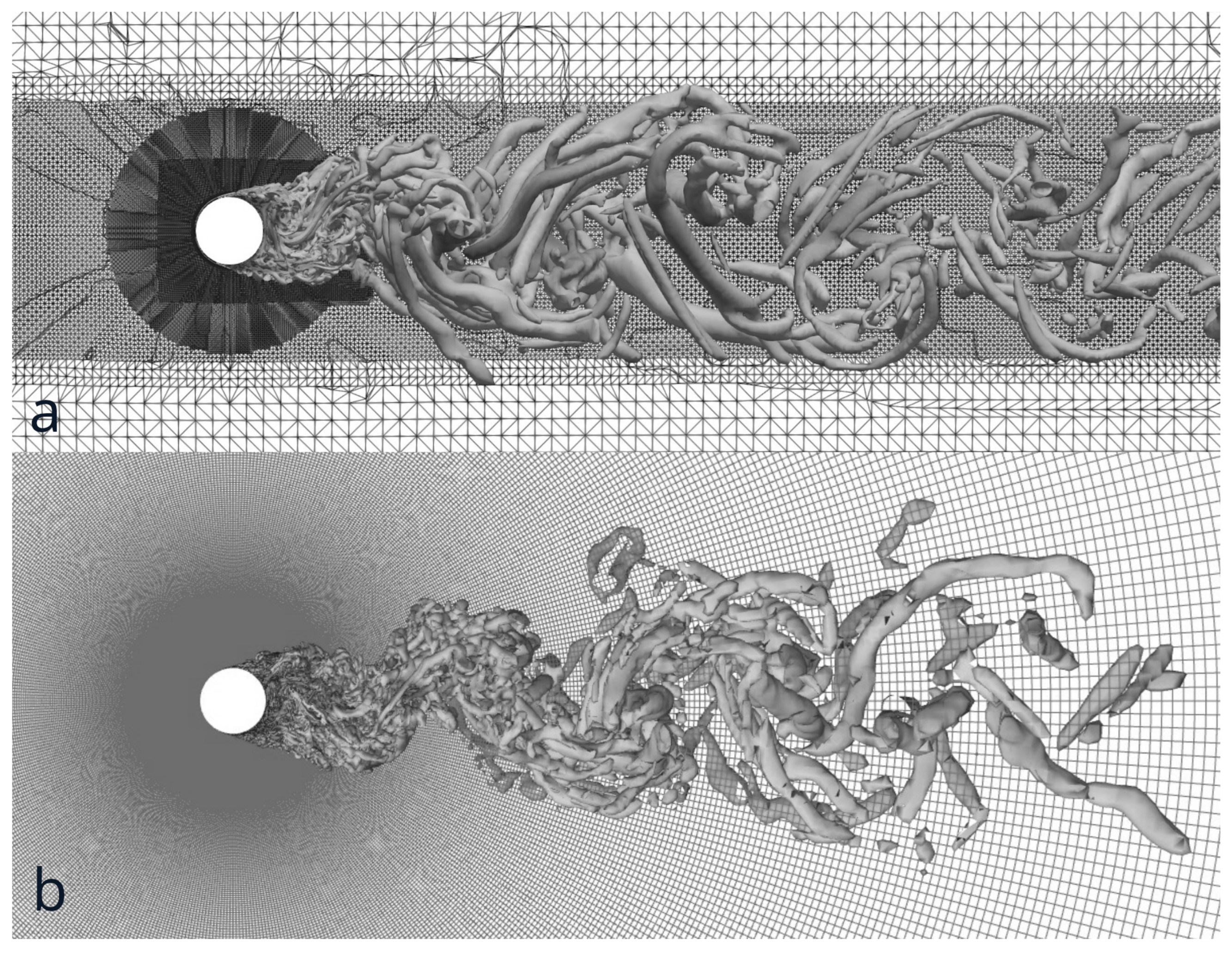
• The present LES (finite-volume method and the dynamic k-equation sub-grid scale model) successfully reproduced the complex physics of the turbulent flow over a circular cylinder, including the Kelvin–Helmholtz and Benard/von Kármán instabilities, the laminar–turbulent transition, development of vortex cores, their downstream convection, and vortex dynamics in the wake.
• In general, satisfactory agreement between LES results obtained using Ansys Fluent and OpenFOAM and experimental data was observed. Discrepancies between them can be attributed to the specifics of numerical simulations (e.g., various computational grids, convective schemes, sub-grid scale models, algorithms, and methods to solve the Navier–Stokes equations) and the techniques used for collecting physical measurements. The location of the laminar–turbulent transition, which is very sensitive to the turbulence intensity of the incoming flow, is critically important.
• The present LES results showed that it is possible to capture complex flow physics for this particular Reynolds number using medium-sized computational grids (up to 25 million cells) generated by different refinement strategies (O-type versus unstructured).
• Differences between LES results computed using single- and double-precision arithmetic implemented in Ansys Fluent were negligible for all integral, local, and spectral characteristics of the turbulent flow. A special run using the concept of mixed-precision arithmetic implemented in OpenFOAM showed satisfactory convergence with the results predicted by Ansys Fluent, indicating a significant degree of consistency between these numerical platforms.
• It is worth noting that an attempt to use OpenFOAM with single-precision arithmetic to predict this turbulent flow failed. It seems that the linear algebra solvers implemented in OpenFOAM are more sensitive to round-off errors and related high-frequency noise.
• Lyapunov stability theory and its metrics were applied to analyze the large-eddy simulation technique using single-precision arithmetic. The numerical methodology using single-precision arithmetic was shown to be stable by Lyapunov.
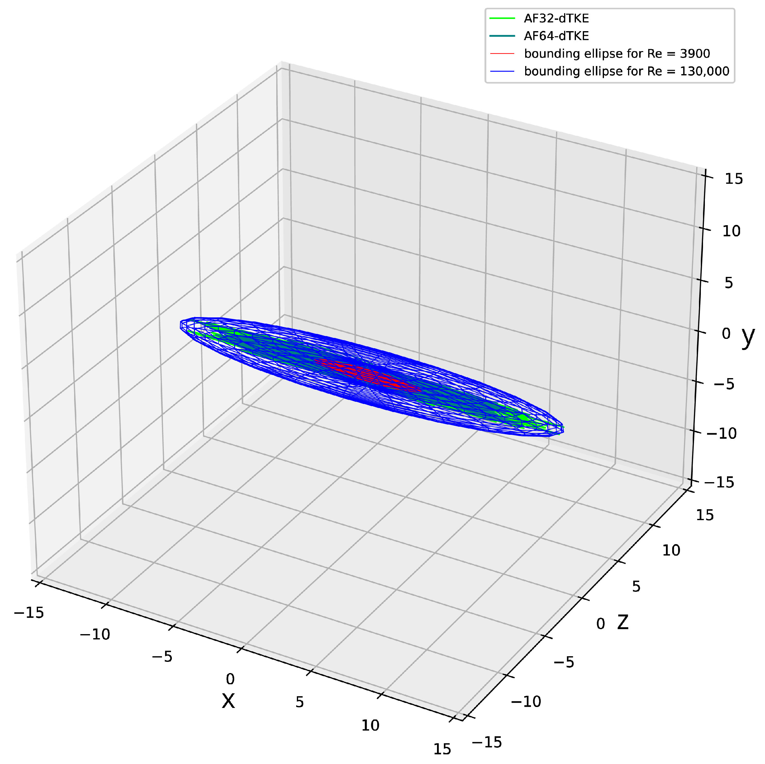
• Under some considerations, LES solutions can be treated as dynamical systems. Their time evolution can be visualized by reconstructed attractors, which can be bounded by simple ellipsoids in three-dimensional space.

The next important step in continuing this work involves the further testing of the numerical methods for the critical and post-critical flow regimes as well as increasing the Mach number to study compressibility effects. It is also essential to analyze the turbulent flow bifurcation and the earlier transition from the sub-critical to critical regimes. This is supported by the observed large dispersion in experimental results for the drag and fluctuating lift coefficients. Additionally, investigating the negative and positive lift coefficients experimentally predicted at transitional Reynolds numbers is of significant importance.

References

1. Lysenko, D.A.; Ertesvåg, I.S.; Rian, K.E. Large-eddy simulation of the flow over a circular cylinder at Reynolds number 3900 using the OpenFOAM toolbox. Flow Turbul. Combust. 2012, 89, 491–518. [Google Scholar] [CrossRef]
2. Lysenko, D.A.; Ertesvåg, I.S.; Rian, K.E. Towards simulation of far-field aerodynamic sound from a circular cylinder using OpenFOAM. Int. J. Aeroacoust. 2014, 13, 141–168. [Google Scholar] [CrossRef]
3. Lysenko, D.A. Free stream turbulence intensity effects on the flow over a circular cylinder at Re = 3900: Bifurcation, attractors and Lyapunov metric. Ocean Eng. 2023, 287, 115787. [Google Scholar] [CrossRef]
4. Lysenko, D.A.; Ertesvåg, I.S.; Rian, K.E. Large-eddy simulation of the flow over a circular cylinder at Reynolds number 2 × 10⁴. Flow Turbul. Combust. 2014, 92, 673–698. [Google Scholar] [CrossRef]
5. Lysenko, D.A.; Ertesvåg, I.S. Reynolds-Averaged, Scale-Adaptive and Large-Eddy Simulations of Premixed Bluff-Body Combustion Using the Eddy Dissipation Concept. Flow Turbul. Combust. 2018, 100, 721–768. [Google Scholar] [CrossRef]
6. Lysenko, D.A.; Ertesvåg, I.S. Assessment of algebraic subgrid scale models for the flow over a triangular cylinder at Re = 45,000. Ocean Eng. 2021, 222, 108559. [Google Scholar] [CrossRef]
7. Lysenko, D.A.; Donskov, M.; Ertesvåg, I.S. Large-eddy simulations of the flow over a semi-circular cylinder at Re = 50,000. Comput. Fluids 2021, 228, 10505. [Google Scholar] [CrossRef]
8. Lysenko, D.A.; Donskov, M.; Ertesvåg, I.S. Large-eddy simulations of the flow past a bluff-body with active flow control based on trapped vortex cells at Re = 50,000. Ocean Eng. 2023, 280, 114496. [Google Scholar] [CrossRef]
9. Breuer, M. A challenging test case for large eddy simulation: High Reynolds number circular cylinder flow. Int. J. Heat Fluid Flow 2000, 21, 648–654. [Google Scholar] [CrossRef]
10. Cao, Y.; Tamura, T. Numerical investigations into effects of three-dimensional wake patterns on unsteady aerodynamic characteristics of a circular cylinder at Re = 1.3 × 10⁵. J. Fluids Struct. 2015, 59, 351–369. [Google Scholar] [CrossRef]
11. Lloyd, T.P.; James, M. Large eddy simulations of a circular cylinder at Reynolds numbers surrounding the drag crisis. Appl. Ocean. Res. 2016, 59, 676–686. [Google Scholar] [CrossRef]
12. Yeon, S.M.; Yang, J.; Stern, F. Large-eddy simulation of the flow past a circular cylinder at sub- to super-critical Reynolds numbers. Appl. Ocean. Res. 2016, 59, 663–675. [Google Scholar] [CrossRef]
13. Plata, M.; Lamballais, E.; Naddei, F. On the performance of a high-order multiscale DG approach to LES at increasing Reynolds number. Comput. Fluids 2019, 194, 104306. [Google Scholar] [CrossRef]
14. Cantwell, B.; Coles, D. An experimental study of entrainment and transport in the turbulent near wake of a circular cylinder. J. Fluid Mech. 1983, 136, 321–374. [Google Scholar] [CrossRef]
15. Roshko, A. On the Drag and Shedding Frequency of Two-Dimensional Bluff Bodies; NACA-TN-3169; National Advisory Committee for Aeronautics: Washington, DC, USA, 1953. [Google Scholar]
16. Delany, K.; Sorensen, N.E. Low-Speed Drag of Cylinders of Various Shapes; NACA-TM-3038; NASA: Washington, DC, USA, 1956. [Google Scholar]
17. Achenbach, E. Distribution of local pressure and skin friction around a circular cylinder in cross-flow up to Re = 5 × 10⁶. J. Fluid Mech. 1968, 34, 625–639. [Google Scholar] [CrossRef]
18. Bearman, P.W. On vortex shedding from a circular cylinder in the critical Reynolds number regime. J. Fluid Mech. 1969, 37, 577–585. [Google Scholar] [CrossRef]
19. Son, J.; Hanratty, T. Velocity gradients at the wall for flow around a cylinder at Reynolds numbers from 5 × 10³ to 105. J. Fluid Mech. 1969, 35, 353–368. [Google Scholar] [CrossRef]
20. Chen, C.F.; Ballengee, D.B. Vortex shedding from circular cylinders in an oscillating freestream. AIAA J. 1971, 9, 340–342. [Google Scholar] [CrossRef]
21. Sadeh, W.Z.; Saharon, D.B. Turbulence Effect on Crossflow Around a Circular Cylinder at Subcritical Reynolds Numbers; NASA-CR-3622; National Advisory Committee for Aeronautics: Washington, DC, USA, 1982. [Google Scholar]
22. Schewe, G. On the force fluctuations acting on a circular cylinder in crossflow from subcritical up to transcritical Reynolds numbers. J. Fluid Mech. 1983, 133, 265–285. [Google Scholar] [CrossRef]
23. Norberg, C. Effects of Reynolds Number and a Low Intensity Freestream Turbulence on the Flow Around a Circular Cylinder; Publication No. 87/2; Chalmers University of Technology: Göteborg, Sweden, 1987. [Google Scholar]
24. Szepessy, S.; Bearman, P.W. Aspect ratio and end plate effects on vortex shedding from a circular cylinder. J. Fluid Mech. 1992, 234, 191–217. [Google Scholar] [CrossRef]
25. Shih, W.C.L.; Wang, C.; Coles, D.; Roshko, A. Experiments on flow past rough circular cylinders at large Reynolds numbers. J. Wind Eng. Ind. Aerodyn. 1993, 49, 351–368. [Google Scholar] [CrossRef]
26. West, G.S.; Apelt, C.J. Measurements of fluctuating pressures and forces on a circular cylinder in the Reynolds number range 104 to 2.5 × 10⁵. J. Fluids Struct. 1993, 7, 227–244. [Google Scholar] [CrossRef]
27. Norberg, C. Flow around rectangular cylinders: Pressure forces and wake frequencies. J. Wind Eng. Ind. Aerodyn. 1993, 49, 187–196. [Google Scholar] [CrossRef]
28. Norberg, C. Flow around a circular cylinder: Aspects of fluctuating lift. J. Fluids Struct. 2001, 15, 459–469. [Google Scholar] [CrossRef]
29. Lim, H.-C.; Lee, S.-J. Flow control of circular cylinders with longitudinal grooved surfaces. AIAA J. 2002, 40, 2027–2036. [Google Scholar] [CrossRef]
30. Wen, P.; Qiu, W. Numerical studies of VIV of a smooth cylinder. In Proceedings of the 27th ITTC Workshop on Wave Run-Up and Vortex Shedding, Nantes, France, 17–18 October 2013. [Google Scholar]
31. Capone, A.; Klein, C.; Felice, F.D.; Miozzi, M. Phenomenology of a flow around a circular cylinder at sub-critical and critical Reynolds numbers. Phys. Fluids 2016, 28, 074101. [Google Scholar] [CrossRef]
32. Brogi, F.; Bnà, S.; Boga, G.; Amati, G.; Esposti Ongaro, T.; Cerminara, M. On floating point precision in computational fluid dynamics using OpenFOAM. Future Gener. Comput. Syst. 2024, 152, 1–16. [Google Scholar] [CrossRef]
33. Karypis, G.; Kumar, V. Multilevel k-way partitioning scheme for irregular graphs. J. Parallel Dist. Comput. 1998, 48, 96–129. [Google Scholar] [CrossRef]
34. Chevalier, C.; Pellegrini, F. PT-Scotch: A tool for efficient parallel graph ordering. Parallel Comput. 2008, 34, 318–331. [Google Scholar] [CrossRef]
35. Geurts, B. Elements of Direct and Large-Eddy Simulation; R.T. Edwards: Philadelphia, PA, USA, 2004. [Google Scholar]
36. Garnier, E.; Adams, N.; Sagaut, P. Large Eddy Simulation for Compressible Flows; Springer: New York, NY, USA, 2009. [Google Scholar]
37. Schumann, U. Subgrid scale model for finite difference simulations of turbulent flows in plane channels and annuli. J. Comput. Phys. 1975, 18, 376–404. [Google Scholar] [CrossRef]
38. Horiuti, K. Large eddy simulation of turbulent channel flow by one-equation modeling. J. Phys. Soc. Jpn. 1985, 54, 2855–2865. [Google Scholar] [CrossRef]
39. Yoshizawa, A. Statistical theory for compressible shear flows, with the application to subgrid modelling. Phys. Fluids 1986, 29, 1416–1429. [Google Scholar] [CrossRef]
40. Sagaut, P. Large Eddy Simulation for Incompressible Flows, 3rd ed.; Springer: Berlin, Germany, 2006. [Google Scholar]
41. ANSYS FLUENT 2021SRb—Theory Guide; Technical Report; Ansys Inc.: Canonsburg, PA, USA, 2021.
42. Weller, H.G.; Tabor, G.; Jasak, H.; Fureby, C. A tensorial approach to computational continuum mechanics using object-oriented techniques. J. Comput. Phys. 1998, 12, 620–631. [Google Scholar] [CrossRef]
43. Issa, R. Solution of the implicitly discretized fluid flow equations by operator splitting. J. Comput Phys. 1986, 62, 40–65. [Google Scholar] [CrossRef]
44. Hutchinson, B.; Raithby, G. A multigrid method based on the additive correction strategy. J. Numer. Heat Transfer 1986, 9, 511–537. [Google Scholar]
45. Wesseling, P.; Oosterlee, C.W. Geometric multigrid with applications to computational fluid dynamics. Comput. Appl. Math. 2001, 128, 311–334. [Google Scholar] [CrossRef]
46. Welch, P. The use of fast Fourier transform for the estimation of power spectra: A method based on time averaging over short, modified periodograms. IEEE Trans. Audio Electroacoust. 1967, 15, 70–73. [Google Scholar] [CrossRef]
47. Kravchenko, A.; Moin, P. Numerical studies of flow over a circular cylinder at Re = 3900. Phys. Fluids 2000, 12, 403–417. [Google Scholar] [CrossRef]
48. Parnaudeau, P.; Carlier, J.; Heitz, D.; Lamballais, E. Experimental and numerical studies of the flow over a circular cylinder at Reynolds number 3900. Phys. Fluids 2008, 20, 085101. [Google Scholar] [CrossRef]
49. Prasad, A.; Williamson, C.H.K. Three-dimensional effects in turbulent bluff-body wakes. J. Fluid Mech. 1997, 343, 235–265. [Google Scholar] [CrossRef]
50. Ong, L.; Wallace, J. The velocity field of the turbulent very near wake of a circular cylinder. Exp. Fluids 1996, 20, 441–453. [Google Scholar] [CrossRef]
51. Ma, X.; Karamanos, G.-S.; Karniadakis, G.E. Dynamics and low-dimensionality of a turbulent near wake. J. Fluid Mech. 2000, 410, 29–65. [Google Scholar] [CrossRef]
52. Shanbhogue, S.J.; Husain, S.; Lieuwen, T. Lean blowoff of bluff body stabilized flames: Scaling and dynamics. Prog. Energy Combust. Sci. 2009, 35, 98–120. [Google Scholar] [CrossRef]
53. Dong, S.; Karniadakis, G.E.; Ekmekci, A.; Rockwell, D. A combined direct numerical simulation particle image velocimetry study of the turbulent air wake. J. Fluid Mech. 2006, 569, 185–207. [Google Scholar] [CrossRef]
54. Bloor, M. The transition to turbulence in the wake of a circular cylinder. J. Fluid Mech. 1964, 19, 290–304. [Google Scholar] [CrossRef]
55. Brun, C.; Aubrun, S.; Goossens, T.; Ravier, P. Coherent structures and their frequency signature in the separated shear layer on the sides of a square cylinder. Flow Turbul. Combust. 2008, 81, 97–114. [Google Scholar] [CrossRef]
56. Trias, F.X.; Gorobets, A.; Oliva, A. Turbulent flow around a square cylinder at Reynolds number 22,000: A DNS study. Comput. Fluids 2015, 123, 87–98. [Google Scholar] [CrossRef]
57. Lander, D.C.; Moore, D.M.; Letchford, C.W.; Amitay, M. Scaling of square-prism shear layers. J. Fluid Mech. 2018, 849, 1096–1119. [Google Scholar] [CrossRef]
58. Moore, D.M.; Letchford, C.W.; Amitay, M. Energetic scales in a bluff body shear layer. J. Fluid Mech. 2019, 875, 543–575. [Google Scholar] [CrossRef]
59. Kourta, A.; Boisson, H.; Chassing, P.; Ha Minh, H. Non-linear interactions and the transition to turbulence in the wake of a circular cylinder. J. Fluid Mech. 1987, 181, 41–161. [Google Scholar] [CrossRef]
60. Mihailovic, J.; Corke, T.C. Three-dimensional instability of the shear layer over a circular cylinder. Phys. Fluids 2019, 9, 3250–3257. [Google Scholar] [CrossRef]
61. Prasad, A.; Williamson, C.H.K. The instability of the shear layer separating from a bluff body. J. Fluid Mech. 1997, 333, 375–402. [Google Scholar] [CrossRef]
62. Rajagopalan, S.; Antonia, R.A. Flow around a circular cylinder - structure of the near wake shear layer. Exp. Fluids 2005, 38, 393–402. [Google Scholar] [CrossRef]
63. Maekawa, T.; Mizuno, S. Flow around the separation point and in the near wake of a circular cylinder. Phys. Fluids 1967, 10, 184–186. [Google Scholar] [CrossRef]
64. Jordan, S. Investigation of the cylinder separated shear-layer physics by large-eddy simulation. Int. J. Heat Fluid Flow 2002, 23, 1–12. [Google Scholar] [CrossRef]
65. Cao, Y.; Tamura, T. Large-eddy simulations of flow past a square cylinder using structured and unstructured grids. Comput. Fluids 2016, 137, 36–54. [Google Scholar] [CrossRef]
66. Nastac, G.; Labahn, J.W.; Magri, L.; Ihme, M. Lyapunov exponent as a metric for assessing the dynamic content and predictability of large-eddy simulations. Phys. Rev. Fluids 2017, 2, 094606. [Google Scholar] [CrossRef]
67. Oseledets, V.I. Multiplicative ergodic theorem. Characteristic Lyapunov exponents of dynamical systems. Tr. Mosk. Mat. Obs. 1968, 19, 179–210. [Google Scholar]
68. Lyapunov, A.M. The general problem of the stability of motion. Int. J. Control 1992, 55, 521–790. [Google Scholar] [CrossRef]
69. Ruelle, D.; Takens, F. On the nature of turbulence. Commun. Math Phys. 1971, 23, 343–344. [Google Scholar] [CrossRef]
70. Alberti, T.; Daviaud, F.; Donner, R.V.; Dubrulle, B.; Faranda, D.; Lucarini, V. Chameleon attractors in a turbulent flow. Chaos Solitons Fractals 2023, 168, 113195. [Google Scholar] [CrossRef]
71. Takens, F. Detecting strange attractors in turbulence. In Dynamical Systems and Turbulence, Warwick 1980; Springer: Berlin/Heidelberg, Germany, 1981; Volume 898, pp. 366–381. [Google Scholar]
72. Sharma, P.; Chung, W.T.; Akoush, B.; Ihme, M. A Review of Physics-Informed Machine Learning in Fluid Mechanics. Energies 2023, 16, 2343. [Google Scholar] [CrossRef]
Figure 1. General view of the unstructured, hexahedral and curvilinear, orthogonal meshes and computational domain ((b,d) and (e,g), respectively), and their frontal view and zoom in the vicinity of cylinder (c,f). x, y and z are Cartesian coordinates in the longitudinal, vertical, and spanwise directions, and θ and r are circumferential and radial coordinates (a).
Fluids 10 00004 g001
Figure 2. Time evolution of the lift (a,c) and drag (b,d) coefficients obtained for OF-TKE, OF-dTKE and AF64-dTKE, AF32-dTKE runs, respectively, during over ≈30 oscillation periods for the flow past a circular cylinder at Re = 130,000.
Fluids 10 00004 g002
Figure 3. Visualization of a vortex shedding downstream from a circular cylinder at Re = 130,000 using the Q-criterion, Q = 10 4 : OF-dTKE (a) and AF64-dTKE (b).
Fluids 10 00004 g003
Figure 4. Probability density distribution (PDF) of the lift coefficient normalized by its root-mean-square value: AF32-dTKE (a), AF64-dTKE (b), OF-TKE (c), and OF-dTKE (d).
Fluids 10 00004 g004
Figure 5. Comparison of the pressure (a) and friction (b) coefficients over the cylinder surface ( θ s = 0 —stagnation point) for the flow over a circular cylinder at Re = 130,000. Note that the present results are not averaged in the spanwise direction in order to show their variation over L z .
Fluids 10 00004 g005
Figure 6. Distribution of the mean streamwise velocity (a) as well as the RMS values of the streamwise (b) and vertical (c) velocity along the central axis for the flow over a circular cylinder at Re = 130,000.
Fluids 10 00004 g006
Figure 7. Radial profiles of the mean streamwise and vertical velocities as well as the mean Reynolds stresses U x U u in the near wake ( x / D = 1.0 , 1.5 , 2.0 ) for the flow over a circular cylinder at Re = 130,000.
Fluids 10 00004 g007
Figure 8. One-dimensional energy spectra of the vertical velocity in the near wake of a circular cylinder (a) and shear layer instability (b) at Re = 130,000. Signals measured at points x / D = 1.5 , y / D = 0 (a) and x / D = 0.15 , y / D = 0.5 (b) with multiple distributions along the span.
Fluids 10 00004 g008
Figure 10. Energy scalogram of wavelet coefficients for the vertical velocity in the wake of circular cylinder in a separated shear layer, calculated using CWT for Re = 3900 , 20,000 and 130,000 (AF64-dTKE run). Energy scalograms for Re = 3900 and Re = 20,000 were computed based on results obtained in [1] and [4], respectively. Here, t * = t U / D is the dimensionless time. The dashed line shows the average frequency of the broadband interval f k h / f v s = 28.9 for Re = 130,000.
Fluids 10 00004 g010
Figure 11. Divergence in streamwise (a), vertical (b), and spanwise (c) velocities between two solutions obtained using single-precision (AF32) and double-precision (AF64) arithmetic for the flow over a circular cylinder at Re = 130,000. The time scale is normalized using the convective time, τ c o n v . The dashed lines represent the linear region, and the dash-dotted lines represent the saturation region.
Fluids 10 00004 g011
Figure 12. Attractors of nonlinear systems AF32-dTKE and AF64-dTKE for the flow over a circular cylinder at Re = 130,000, as well as their bounding ellipsoids, in the three-dimensional space. For the sake of completeness, similar results for Re = 3900 [3] are presented.
Fluids 10 00004 g012
Figure 13. One -dimensional energy spectra of the vertical velocity in the near wake of a circular cylinder (a) and shear layer instability (b) for the flow over a circular cylinder at Re = 130,000. Signals measured at points x / D = 1.5 , y / D = 0 (a) and x / D = 0.15 , y / D = 0.5 (b).
Fluids 10 00004 g013
Figure 14. Radial profiles of the mean Reynolds stresses U x U u in the near wake ( x / D = 1.0 , 1.5 , 2.0 ) for the flow over a circular cylinder at Re = 130,000.
Fluids 10 00004 g014
Figure 15. The mean drag (a), lift (b), fluctuating lift (c) coefficients, separation angle (d), mean base pressure coefficient (e), and Strouhal number (f) as functions of the Reynolds number for the flow over a circular cylinder.
Fluids 10 00004 g015